Point process models for sequence detection in high-dimensional neural spike trains
←
→
Page content transcription
If your browser does not render page correctly, please read the page content below
Point process models for sequence detection in
           high-dimensional neural spike trains

               Alex H. Williams                             Anthony Degleris
            Department of Statistics                Department of Electrical Engineering
              Stanford University                          Stanford University
              Stanford, CA 94305                           Stanford, CA 94305
           ahwillia@stanford.edu                        degleris@stanford.edu

                 Yixin Wang                                 Scott W. Linderman
            Department of Statistics                       Department of Statistics
              Columbia University                            Stanford University
             New York NY 10027                               Stanford, CA 94305
          yixin.wang@columbia.edu                     scott.linderman@stanford.edu

                                             Abstract
         Sparse sequences of neural spikes are posited to underlie aspects of working
         memory [1], motor production [2], and learning [3, 4]. Discovering these sequences
         in an unsupervised manner is a longstanding problem in statistical neuroscience
         [5–7]. Promising recent work [4, 8] utilized a convolutive nonnegative matrix
         factorization model [9] to tackle this challenge. However, this model requires spike
         times to be discretized, utilizes a sub-optimal least-squares criterion, and does
         not provide uncertainty estimates for model predictions or estimated parameters.
         We address each of these shortcomings by developing a point process model that
         characterizes fine-scale sequences at the level of individual spikes and represents
         sequence occurrences as a small number of marked events in continuous time. This
         ultra-sparse representation of sequence events opens new possibilities for spike
         train modeling. For example, we introduce learnable time warping parameters to
         model sequences of varying duration, which have been experimentally observed in
         neural circuits [10]. We demonstrate these advantages on experimental recordings
         from songbird higher vocal center and rodent hippocampus.

1   Introduction
Identifying interpretable patterns in multi-electrode recordings is a longstanding and increasingly
pressing challenge in neuroscience. Depending on the brain area and behavioral task, the activity
of large neural populations may be low-dimensional as quantified by principal components analysis
(PCA) or other latent variable models [11–23]. However, many datasets do not conform to these
modeling assumptions and instead exhibit high-dimensional behaviors [24]. Neural sequences are
an important example of high-dimensional structure: if N neurons fire sequentially with no overlap,
the resulting dynamics are N -dimensional and cannot be efficiently summarized by PCA or other
linear dimensionality reduction methods [4]. Such sequences underlie current theories of working
memory [1, 25], motor production [2], and memory replay [10]. More generally, neural sequences
are seen as flexible building blocks for learning and executing complex neural computations [26–28].
Prior Work In practice, neural sequences are usually identified in a supervised manner by correlat-
ing neural firing with salient sensory cues or behavioral actions. For example, hippocampal place
cells fire sequentially when rodents travel down a narrow hallway, and these sequences can be found

34th Conference on Neural Information Processing Systems (NeurIPS 2020), Vancouver, Canada.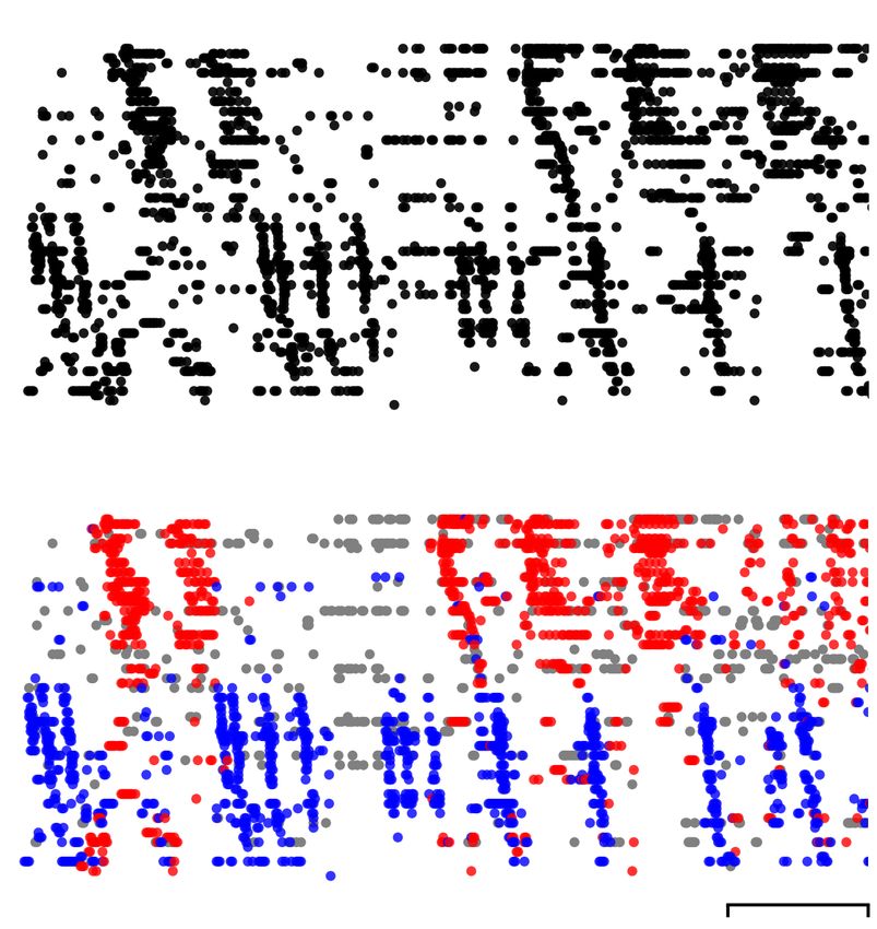
by averaging spikes times over multiple traversals of the hallway. After identifying this sequence
on a behavioral timescale lasting seconds, a template matching procedure can be used to show that
these sequences reoccur on compressed timescales during wake [29] and sleep [30]. In other cases,
sequences can be identified relative to salient features of the local field potential (LFP; [31, 32]).
Developing unsupervised alternatives that directly extract sequences from multineuronal spike trains
would broaden the scope of this research and potentially uncover new sequences that are not linked
to behaviors or sensations [33]. Several works have shown preliminary progress in this direction
Maboudi et al. [34] proposed fitting a hidden Markov model (HMM) and then identifying sequences
from the state transition matrix. Grossberger et al. [35] and van der Meij & Voytek [36] apply
clustering to features computed over a sliding window. Others use statistics such as time-lagged
correlations to detect sequences and other spatiotemporal patterns in a bottom-up fashion [6, 7].
In this paper, we develop a Bayesian point process modeling generalization of convolutive nonnegative
matrix factorization (convNMF; [9]), which was recently used by Peter et al. [8] and Mackevicius
et al. [4] to model neural sequences. Briefly, the convNMF model discretizes each neuron’s spike
train into a vector of B time bins,PxRn ∈ R+ for neuron n, and approximates this collection
                                            B
                                                                                              of vectors
as a sum of convolutions, xn ≈ r=1 wn,r ∗ hr . The model parameters (wn,r ∈ RL+ and hr ∈ RB           +)
are optimized with respect to a least-squares criterion. Each component of the model, indexed by
r ∈ {1, . . . , R}, consists of a neural factor, Wr ∈ RN +
                                                          ×L
                                                              and a temporal factor, hr . The neural
factor encodes a spatiotemporal pattern of neural activity over L time bins (which is hoped to be
sequence), while the temporal factor indicates the times at which this pattern of neural activity occurs.
A total of R motifs or sequence types, each corresponding to a different component, are extracted by
this model.
There are several compelling features of this approach. Similar to classical nonnegative matrix
factorization [37], and in contrast to clustering methods, convNMF captures sequences with overlap-
ping groups of neurons by an intuitive “parts-based” representation. Indeed, convNMF uncovered
overlapping sequences in experimental data from songbird higher vocal center (HVC) [4]. Further, if
the same sequence is repeated with different peak firing rates, convNMF can capture this by varying
the magnitude of the entries in hr , unlike many clustering methods. Finally, convNMF efficiently
pools statistical power across large populations of neurons to identify sequences even when the
correlations between temporally adjacent neurons are noisy—other methods, such as HMMs and
bottom-up agglomerative clustering, require reliable pairwise correlations to string together a full
sequence.
Our Contributions We propose a point process model for neural sequences (PP-Seq) which extends
and generalizes convNMF to continuous time and uses a fully probabilistic Bayesian framework. This
enables us to better quantify uncertainty in key parameters—e.g. the overall number of sequences the
times at which they occur—and also characterize the data at finer timescales—e.g. whether individual
spikes were evoked by a sequence. Most importantly, by achieving an extremely sparse representation
of sequence event times, the PP-Seq model enables a variety of model extensions that are not easily
incorported into convNMF or other common methods. We explore one such extension that introduces
time warping factors to model sequences of varying duration, as is often observed in neural data [10].
Though we focus on applications in neuroscience, our approach could be adapted to other temporal
point processes, which are a natural framework to describe data that are collected at irregular intervals
(e.g. social media posts, consumer behaviors, and medical records) [38, 39]. We draw a novel
connection between Neyman-Scott processes [40], which encompass PP-Seq and other temporal
point process models as special cases, and mixture of finite mixture models [41]. Exploiting this
insight, we develop innovative Markov chain Monte Carlo (MCMC) methods for PP-Seq.

2     Model

2.1   Point Process Models and Neyman-Scott Processes

Point processes are probabilistic models that generate discrete sets {x1 , x2 , . . .} , {xs }Ss=1 over
some continuous space X . Each member of the set xs ∈ X is called an “event.” A Poisson
process [42] is a point process which satisfies three properties. First, the number of events falling
within any region V ⊂ X is Poisson distributed.
                                        R          Second, there exists a function λ(x) : X 7→ R+ ,
called the intensity function, for which V λ(x) dx equals the expected number of events in V . Third,

                                                   2
A Neyman-Scott Process
(2D example, no background) B PP-Seq (1D Neyman-Scott Process, with marked events)
z3
raw spike times z2
(observed events) z1 θ∅ θr
Ak r 2 = 2
r1 = 1 r3 = 1 R
neurons
zk
λ1 (t) zk
...
xs spikes attributed
to latent events
λn (t) bn,rk an,rk x0s xks
neurons
Sk ∼Po( g(x))
...
X
Latent Events S0 ∼ Po(λ∅ T ) Sk ∼ Po(Ak )
Observed Events K ∼ Po( Z
λ(z))
λN (t) cn,rk
time τ1 τ2 τ3 K ∼ Po(ψT )
Figure 1: (A) Example of a Neyman-Scott process over a 2D region. Latent events (purple dots)
are first sampled from a homogeneous Poisson process. Each latent event then spawns a number of
nearby observed events (gray dots), according to an inhomogeneous Poisson process. (B) A spike
train can be modeled as a Neyman-Scott process with marked events over a 1D interval representing
time. Latent events (zk ; sequences) evoke observed events (xs ; spikes) ordered in a sequence. An
example with K = 3 latent events evoking R = 2 different sequence types (blue & red) is shown.
the number of events in non-overlapping regions of X are independent. A Poisson process is said to
be homogeneous when λ(x) = c for some constant c. Finally, a marked point process extends the
usual definition of a point process to incorporate additional information into each event. A marked
point process on X generates random tuples xs = (x̃s , ms ), where x̃s ∈ X represents the random
location and ms ∈ M is the additional “mark” specifying metadata associated with event s. See
Supplement A for further background details and references.
Neyman-Scott Processes [40] use Poisson processes as building blocks to model clustered data.
To simulate a Neyman-Scott process, first sample a set of latent events {zk }K k=1 ⊂ Z from an
initial Poisson process with intensity function λ(z) : Z 7→
R R+ . Thus, the number of latent events
is a Poisson-distributed random variable, K ∼ Poisson( Z λ(z)dz). Given the latent events, the
S
observed events {xP s }s=1 are drawn from a second Poisson process with conditional intensity func-
∅ K
tion λ(x) = λ + k=1 g(x; zk ). The nonnegative functions g(x; zk ) can be thought of as impulse
responses—each latent event adds to the rate of observed events, and stochastically generates some
number of observed offspring events. Finally, the scalar parameter λ∅ > 0 specifies a “background”
rate; thus, if K = 0, the observations follow a homogeneous Poisson process with intensity λ∅ .
A simple example of a Neyman-Scott Process in R2 is shown in fig. 1A. Latent events (purple dots)
are first drawn from a homogenous Poisson process and specify the cluster centroids. Each latent
event induces an isotropic Gaussian impulse response. Observed events (gray dots) are then sampled
from a second Poisson process, whose intensity function is found by summing all impulse responses.
Importantly, we do not observe the number of latent events nor their locations. As described below,
we use probabilistic inference to characterize this unobserved structure. A key idea is to attribute
each observed event to a latent cause (either one of the latent events or the background process); these
attributions are valid due to the additive nature of the latent intensity functions and the superposition
principle of Poisson processes (see Supplement A). From this perspective, inferring the set of latent
events is similar to inferring the number and location of clusters in a nonparametric mixture model.
2.2 Point Process Model of Neural Sequences (PP-Seq)
We model neural sequences as a Neyman-Scott process with marked events in a model we call
PP-Seq. Consider a dataset with N neurons, emitting a total of S spikes over a time interval [0, T ].
This can be encoded as a set of S marked spike times—the observed events are tuples xs = (ts , ns )
specifying the time, ts ∈ [0, T ], and neuron, ns ∈ {1 , . . . , N }, of each spike. Sequences corre-
spond to latent events, which are also tuples zk = (τk , rk , Ak ) specifying the time, τk ∈ [0, T ],
type, rk ∈ {1 , . . . , R}, and amplitude, Ak > 0 of the sequence. The hyperparameter R specifies the
number of recurring sequence types, which is analogous to the number of components in convNMF.
To draw samples from the PP-Seq model, we first sample sequences (i.e., latent events) from a
Poisson process with intensity λ(z) , λ(τ, r, A) = ψ πr Ga(A; α, β). Here, ψ > 0 sets the rate at
3which sequences occur within the data, π ∈ ∆R sets the probability of the R sequence types, and α, β
parameterize a gamma density which models the sequence amplitude, A. Note that the number
of sequence events is a Poisson-distributed random variable, K ∼ Poisson(ψT ), where the rate
parameter ψT is found by integrating λ(z) over all sequence types, amplitudes, and times.
Conditioned on the set of K sequence events, the firing rate of neuron n is given by a sum of
nonnegative impulse responses:
K
X
λn (t) = λ∅
n + gn (t; zk ). (1)
k=1
We assume these impulse responses vary across neurons and follow a Gaussian form:
gn (t; zk ) = Ak · anrk · N (t | τk + bnrk , cnrk ), (2)
where N (t | µ, σ 2 ) denotes a Gaussian density. The parameters ar = (a1r , . . . , aN r ) ∈ ∆N ,
bnr ∈ R, and cnr ∈ R+ correspond to the weight, latency, and width, respectively, of neurons’
firing rates in sequences of type r. Since the firing rate is a sum of non-negative impulse responses,
the superposition principle of Poisson processes (see Supplement A) implies that we can view the
data as a union of “background” spikes and “induced” spikes from each sequence, justifying the
connection to clustering. The expected number of spikes induced by sequence k is:
XN Z T XN Z ∞
gn (t; zk )dt ≈ gn (t; zk )dt = Ak , (3)
n=1 0 n=1 −∞
and thus we may view Ak as the amplitude of sequence event k.
Figure 1B schematizes a simple case containing K = 3 sequence events and R = 2 sequence types.
A complete description of the model’s generative process is provided in Supplement B, but it can be
summarized by the graphical model in fig. 1B, where we have global parameters Θ = (θ∅ , {θr }R r=1 )
∅ N
with θr = (ar , {bnr }N N
n=1 , {cnr }n=1 ) for each sequence type, and θ∅ = {λn }n=1 for the background
process. We place weak priors on each parameter: the neural response weights {anr }N n=1 follow a
Dirichlet prior for each sequence type, and (bnr , cnr ) follows a normal-inverse-gamma prior for every
neuron and sequence type. The background rate, λ∅ n , follows a gamma prior. We set the sequence
event rate, ψ, to be a fixed hyperparameter, though this assumption could be relaxed.
Time-warped sequences PP-Seq can be extended to model more diverse sequence patterns by
using higher-dimensional marks on the latent sequences. For example, we can model variability
in sequence duration by introducing a time warping factor, ωk > 0, to each sequence event and
changing eq. (2) to,
gn (t; zk ) = Ak · an,rk · N (t | τk + ωk bn,rk , ωk2 cn,rk ). (4)
This has the effect of linearly compressing or stretching each sequence in time (when ωk < 1
or ωk > 1, respectively). Such time warping is commonly observed in neural data [43, 44],
and indeed, hippocampal sequences unfold ∼15-20 times faster during replay than during lived
experiences [10]. We characterize this model in Supplement E and demonstrate its utility below.
In principle, it is equally possible to incorporate time warping into discrete time convNMF. However,
R×B
since convNMF involves a dense temporal factor matrix H ∈ R+ , the most straightforward
extension would be to introduce a time warping factor for each component r ∈ {1, . . . , R} and each
time bin b ∈ {1, . . . , B}. This results in O(RB) new trainable parameters, which poses non-trivial
challenges in terms of computational efficiency, overfitting, and human interpretability. In contrast,
PP-Seq represents sequence events as a set of K latent events in continuous time. This ultra-sparse
representation of sequence events (since K
RB) naturally lends itself to modeling additional
sequence features since this introduces only O(K) new parameters.
3 Collapsed Gibbs Sampling for Neyman-Scott Processes
Developing efficient algorithms for parameter inference in Neyman-Scott process models is an area of
active research [45–48]. To address this challenge, we developed a collapsed Gibbs sampling routine
for Neyman-Scott processes, which encompasses the PP-Seq model as a special case. The method
4resembles “Algorithm 3” of Neal [49]—a well-known approach for sampling from a Dirichlet process
mixture model—and the collapsed Gibbs sampling algorithm for “mixture of finite mixtures” models
developed by Miller et al. [41]. The idea is to partition observed spikes into background spikes
and spikes induced by latent sequences, integrating over the sequence times, types, and amplitudes.
Starting from an initial partition, the sampler iterates over individual spikes and probabilistically
re-assigns them to (a) the background, (b) one of the remaining sequences, or (c) to a new sequence.
The number of sequences in the partition, K ∗ , changes as spikes are removed and re-assigned; thus,
the algorithm is able to explore the full trans-dimensional space of partitions.
The re-assignment probabilities are determined by the prior distribution of partitions under the
Neyman-Scott process and by the likelihood of the induced spikes assigned to each sequence. We
state the conditional probabilities below and provide a full derivation in Supplement D. Let K ∗ denote
the number of sequences in the current partition after spike xs has been removed from its current
assignment. (Note that the number of latent sequences K may exceed K ∗ if some sequences produce
zero spikes.) Likewise, let us denote the sequence assignment of the s-th spike, where us = 0
indicates assignment to the background process and us ∈ {1, . . . , K ∗ } indicates assignment to one
of the latent sequence events. Finally, let Xk = {xs0 : us0 = k, s0 6= s} denote the spikes in the k-th
cluster, excluding xs , and let Sk = |Xk | denote its size. The conditional probability of the partition
under the possible assignments of spike xs are,
∗
∅
p(us = 0 | xs , {Xk }K
k=1 , Θ) ∝ (1 + β) λns (5)
" R #
X
K∗
p(us = k | xs , {Xk }k=1 , Θ) ∝ (α + Sk ) p(rk | Xk ) ans rk p(ts | Xk , rk , ns ) (6)
rk =1
α R
X
∗ ∗ β
p(us = K + 1 | xs , {Xk }K
k=1 , Θ) ∝α ψ πr ans r (7)
1+β r=1
The sampling algorithm iterates over all spikes xs ∈ {x1 , . . . , xS } and updates their assignments
holding the other spikes’ assignments fixed. The probability of assigning spike xs to an existing
cluster marginalizes the time, type, and amplitude of the sequence, resulting in a collapsed Gibbs
sampler [49, 50]. The exact form of the posterior probability p(rk | Xk ) and the parameters of the
posterior predictive p(ts | Xk , rk , ns ) in eq. (6) are given in Supplement C.
After attributing each spike to a latent cause, it is straightforward to draw samples over the remaining
∗
model parameters—the latent sequences {zk }K k=1 and global parameters Θ. Given the spikes and
assignments {xs , us }Ss=1 , we sample the sequences (i.e. their time, amplitude, types, etc.) from
the closed-form conditional p(zk | {xs : us = k}, Θ). Given the sequences and spikes, we sample
∗
the conditional distribution on global parameters p(Θ | {zk }K S
k=1 , {xs , us }s=1 ). Under conjugate
formulations, these updates are straightforward. With these steps, the Markov chain targets the
posterior distribution on model parameters and partitions. Complete derivations are in Supplement D.
Improving MCMC mixing times The intensity of sequence amplitudes Ak is proportional to the
gamma density Ga(Ak ; α, β), and these hyperparameters affect the mixing time of the Gibbs sampler.
Intuitively, if there is little probability of low-amplitude sequences, the sampler is unlikely to create
new sequences and is therefore slow to explore different partitions of spikes.1 If, on the other hand,
the variance of Ga(α, β) is large relative to the mean, then the probability of forming new clusters is
non-negligible and the sampler tends to mix more effectively. Unfortunately, this latter regime is also
probably of lesser scientific interest, since neural sequences are typically large in amplitude—they
can involve many thousands of cells, each potentially contributing a small number of spikes [2, 28].
To address this issue, we propose an annealing procedure to initialize the Markov chain. We fix the
mean of Ak and adjust α and β to slowly lower variance of amplitude distribution. Initially, the
sampler produces many small clusters of spikes, and as we lower the variance of Ga(α, β) to its
target value, the Markov chain typically combines these clusters into larger sequences. We further
improve performance by interspersing “split-merge” Metropolis-Hastings updates [51, 52] between
Gibbs sweeps (see Supplement D.6). Finally, though we have not found it necessary, one could use
convNMF to initialize the MCMC algorithm.
1
This problem is common to other nonparametric Bayesian mixture models as well [41, e.g.].
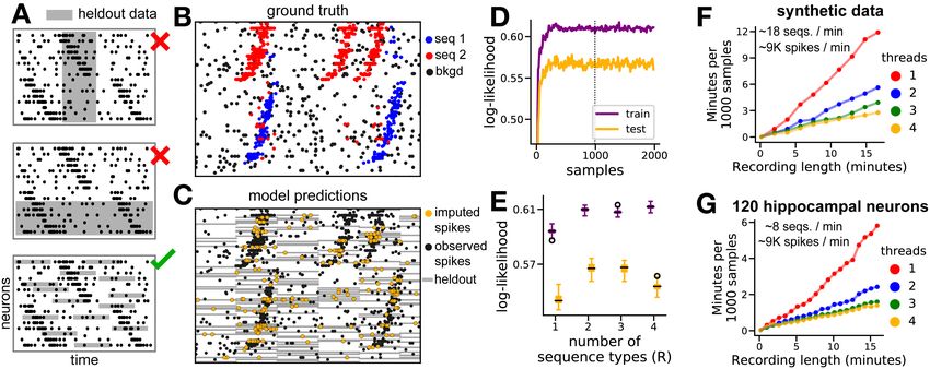
5Figure 2: (A) Schematic of train/test partitions. We propose a speckled holdout pattern (bottom). (B)
A subset of a synthetic spike train containing two sequences types. (C) Same data, but with grey
regions showing the censored test set and yellow dots denoting imputed spikes. (D) Log-likelihood
over Gibbs samples; positive values denote excess nats per unit time relative to a homogeneous
Poisson process baseline. (E) Box plots showing range of log-likelihoods on the train and test sets for
different choices of R; cross-validation favors R = 2, in agreement with the ground truth shown in
panel B. (F-G) Performance benefits of parallel MCMC on synthetic and experimental neural data.
Parallel MCMC Resampling the sequence assignments is the primary computational bottleneck
for the Gibbs sampler. One pass over the data requires O(SKR) operations, which quickly becomes
costly when the operations are serially executed. While this computational cost is manageable for
many datasets, we can improve performance substantially by parallelizing the computation [53].
Given P processors and a spike train lasting T seconds, we divide the dataset into intervals last-
ing T /P seconds, and allocate one interval per processor. The current global parameters, Θ, are
first broadcast to all processors. In parallel, the processors update the sequence assignments for
their assigned spikes, and then send back sufficient statistics describing each sequence. After these
sufficient statistics are collected on a single processor, the global parameters are re-sampled and then
broadcast back to the processors to initiate another iteration. This algorithm introduces some error
since clusters are not shared across processors. In essence, this introduces erroneous edge effects if
a sequence of spikes is split across two processors. However, these errors are negligible when the
sequence length is much less than T /P , which we expect is the practical regime of interest.
4 Experiments
4.1 Cross-Validation and Demonstration of Computational Efficiency
We evaluate model performance by computing the log-likelihood assigned to held-out data. Partition-
ing the data into training and testing sets must be done somewhat carefully—we cannot withhold
time intervals completely (as in fig. 2A, top) or else the model will not accurately predict latent
sequences occurring in these intervals; likewise, we cannot withhold individual neurons completely
(as in fig. 2A, middle) or else the model will not accurately predict the response parameters of those
held out cells. Thus, we adopt a “speckled” holdout strategy [54] as diagrammed at the bottom of
fig. 2A. We treat held-out spikes as missing data and sample them as part of the MCMC algorithm.
(Their conditional distribution is given by the PP-Seq generative model.) This approach involving a
speckled holdout pattern and multiple imputation of missing data may be viewed as a continuous
time extension of the methods proposed by Mackevicius et al. [27] for convNMF.
Panels B-E in fig. 2 show the results of this cross-validation scheme on a synthetic dataset with R = 2
sequence types. The predictions of the model in held-out test regions closely match the ground
truth—missing spikes are reliably imputed when they are part of a sequence (fig. 2C). Further, the
likelihood of the train and test sets improves over the course of MCMC sampling (fig. 2D), and can
be used as a metric for model comparison—in agreement with the ground truth, test performance
plateaus for models containing greater than R = 2 sequence types (fig. 2E).
6A raw data (deconvolved spikes)
B D
convNMF
75 neurons
binned and smoothed data
PP-seq
neurons re-sorted by model
C E
re-sorted neurons
prob.
spikes labeled by model
model reconstruction
high
activity
background sequence 1 3s low
sequence 2
Figure 3: Zebra Finch HVC data. (A) Raw spike train (top) and sequences revealed by PP-Seq
(left) and convNMF (right). (B) Box plots summarizing samples from the posterior on number of
sequences, K, derived from three independent MCMC chains. (C) Co-occupancy matrix summarizing
probabilities of spike pairs belonging to the same sequence. (D) Credible intervals for evoked
amplitudes for sequence type 1 (red) and 2 (blue). (E) Credible intervals for response offsets (same
order and coloring as D). Estimates are suppressed for small-amplitude responses (gray dots).
Finally, to be of practical utility, the algorithm needs to run in a reasonable amount of time. Figure 2G
shows that our Julia [55] implementation can fit a recording of 120 hippocamapal neurons with
hundreds of thousands of spikes in a matter of minutes, on a 2017 MacBook Pro (3.1 GHz Intel Core
i7, 4 cores, 16 GB RAM). Run-time grows linearly with the number of spikes, as expected, but even
with a single thread it only takes six minutes to perform 1000 Gibbs sweeps on a 15-minute recording
with ∼ 1.3 × 10⁵ spikes. With parallel MCMC, this laptop performs the same number of sweeps in
under two minutes. Our open-source implementation is available at:
https://github.com/lindermanlab/PPSeq.jl.
4.2 Zebra Finch Higher Vocal Center (HVC)
We first applied PP-Seq to a recording of HVC premotor neurons in a zebra finch,2 which generate
sequences that are time-locked to syllables in the bird’s courtship song. Figure 3A qualitatively
compares the performance of convNMF and PP-Seq. The raw data (top panel) shows no visible spike
patterns; however, clear sequences are revealed by sorting the neurons lexographically by preferred
sequence type and the temporal offset parameter inferred by PP-Seq. While both models extract
similar sequences, PP-Seq provides a finer scale annotation of the final result, providing, for example,
attributions at the level of individual spikes to sequences (bottom left of fig. 3A).
Further, PP-Seq can quantify uncertainty in key parameters by considering the full sequence of
MCMC samples. Figure 3B summarizes uncertainty in the total number of sequence events, i.e. K,
over three independent MCMC chains with different random seeds—all chains converge to similar
estimates; the uncertainty is largely due to the rapid sequences (in blue) shown in panel A. Figure 3C
displays a symmetric matrix where element (i, j) corresponds to the probability that spike i and
spike j are attributed to same sequence. Finally, fig. 3D-E shows the amplitude and offset for each
neuron’s sequence-evoked response with 95% posterior credible intervals. These results naturally fall
out of the probabilistic construction of the PP-Seq model, but have no obvious analogue in convNMF.
4.3 Time Warping Extension and Robustness to Noise
Songbird HVC is a specialized circuit that generates unusually clean and easy-to-detect sequences. To
compare the robustness of PP-Seq and convNMF under more challenging circumstances, we created a
simple synthetic dataset with R = 1 sequence type and N = 100 neurons. We varied four parameters
to manipulate the difficulty of sequence extraction: the rate of background spikes, λ∅ n (“additive
2
These data are available at http://github.com/FeeLab/seqNMF; originally published in [4].
7A B E
PP-Seq
convNMF
C D F
Figure 4: PP-Seq is more robust to various forms of noise than convNMF. (A-D) Comparison of
PP-Seq and convNMF to detect sequence times in synthetic data with varying amounts of noise.
Panel D shows the performance of the time-warped variant of PP-Seq (see eq. (4)). (E) convNMF
reconstruction of a spike train containing sequences with 9-fold time warping. (F) Performance of
time-warped PP-Seq (see eq. (4)) on the same data as panel E.
noise,” fig. 4A), the expected value of sequence amplitudes, Ak (“participation noise”, fig. 4B), the
expected variance of the Gaussian impulse responses, cnr (“jitter noise”, fig. 4C), and, finally, the
maximal time warping coefficient (see eq. (4); fig. 4D). All simulated datasets involved sequences
with low spike counts (E[Ak ] < 100 spikes). In this regime, the Poisson likelihood criterion used by
PP-Seq is better matched to the statistics of the spike train. Since convNMF optimizes an alternative
loss function (squared error instead of Poisson likelihood) we compared the models by their ability
to extract the ground truth sequence event times. Using area under reciever operating characteriztic
(ROC) curves as a performance metric (see Supplement F.1), we see favorable results for PP-Seq as
noise levels are increased.
We demonstrate the abilities of time-warped PP-Seq further in fig. 4E-F. Here, we show a synthetic
dataset containing sequences with 9-fold variability in their duration, which is similar to levels
observed in some experimental systems [10]. While convNMF fails to reconstruct many of these
warped sequences, the PP-Seq model identifies sequences that are closely matched to ground truth.
4.4 Rodent Hippocampal Sequences
Finally, we tested PP-Seq and its time warping variant on a hippocampal recording in a rat making
repeated runs down a linear track.3 This dataset is larger (T ≈ 16 minutes, S = 137,482) and
contains less stereotyped sequences than the songbird data. From prior work [56], we expect to see
two sequences with overlapping populations of neurons, corresponding to the two running directions
on the track. PP-Seq reveals these expected sequences in an unsupervised manner—i.e. without
reference to the rat’s position—as shown in fig. 5A-C.
We performed a large cross-validation sweep over 2,000 random hyperparameter settings for this
dataset (see Supplement F.2). This confirmed that models with R = 2 sequence performed well in
terms of heldout performance (fig. 5D). Interestingly, despite variability in running speeds, this same
analysis did not show a consistent benefit to including larger time warping factors into the model
(fig. 5E). Higher performing models were characterized by larger sequence amplitudes, i.e. larger
values of E[Ak ] = α/β, and smaller background rates, i.e. smaller values of λ∅ . Other parameters
had less pronounced effects on performance. Overall, these results demonstrate that PP-Seq can
be fruitfully applied to large-scale and “messy” neural datasets, that hyperparameters can be tuned
by cross-validation, and that the unsupervised learning of neural sequences conforms to existing
scientific understanding gained via supervised methods.
3
These data are available at http://crcns.org/data-sets/hc/hc-11; originally published in [56].
8A D E F
validation LL
validation LL
validation LL
B
G H I
validation LL
validation LL
validation LL
C
25 s
Figure 5: Automatic detection of place coding sequences in rat hippocampus. (A) Raw spike train
(∼20% of the full dataset is shown). Blue and red arrowheads indicate when the mouse reaches the
end of the track and reverses direction. (B) Neurons re-sorted by PP-Seq (with R = 2). (C) Sequences
annotated by PP-Seq. (D-I) Validation log-likelihoods as a function of hyperparameter value. Each
boxplot summarizes the 50 highest scoring models, randomly sampling the other hyperparameters.
5 Conclusion
We proposed a point process model (PP-Seq) inspired by convolutive NMF [4, 8, 9] to identify neural
sequences. Both models approximate neural activity as the sum of nonnegative features, drawn from
a fixed number of spatiotemporal motif types. Unlike convNMF, PP-Seq restricts each motif to
be a true sequence—the impulse responses are Gaussian and hence unimodal. Further, PP-Seq is
formulated in a probabilistic framework that better quantifies uncertainty (see fig. 3) and handles
low firing rate regimes (see fig. 4). Finally, PP-Seq produces an extremely sparse representation of
sequence events in continuous time, opening the door to a variety of model extensions including the
introduction of time warping (see fig. 4F), as well as other possibilities like truncated sequences and
“clusterless” observations [57], which could be explored in future work.
Despite these benefits, fitting PP-Seq involves a tackling a challenging trans-dimensional inference
problem inherent to Neyman-Scott point processes. We took several important steps towards over-
coming this challenge by connecting these models to a more general class of Bayesian mixture
models [41], developing and parallelizing a collapsed Gibbs sampler, and devising an annealed
sampling approach to promote fast mixing. These innovations are sufficient to fit PP-Seq on datasets
containing hundreds of thousands of spikes in just a few minutes on a modern laptop.
Acknowledgements
A.H.W. received funding support from the National Institutes of Health BRAIN initiative
(1F32MH122998-01), and the Wu Tsai Stanford Neurosciences Institute Interdisciplinary Scholar
Program. S.W.L. was supported by grants from the Simons Collaboration on the Global Brain (SCGB
697092) and the NIH BRAIN Initiative (U19NS113201 and R01NS113119). We thank the Stanford
Research Computing Center for providing computational resources and support that contributed to
these research results.
Broader Impact
Understanding neural computations in biological systems and ultimately the human brain is a
grand and long-term challenge with broad implications for human health and society. The field
of neuroscience is still taking early and incremental steps towards this goal. Our work develops a
general-purpose, unsupervised method for identifying an important structure—neural sequences—
which have been observed in a variety of experimental datasets and have been studied extensively by
theorists. This work will serve to advance this growing understanding by providing new analytical
tools for neuroscientists. We foresee no immediate impacts, positive or negative, concerning the
general public.
9References
[1] Mark S Goldman. “Memory without feedback in a neural network”. Neuron 61.4 (2009),
pp. 621–634.
[2] Richard H R Hahnloser, Alexay A Kozhevnikov, and Michale S Fee. “An ultra-sparse code
underlies the generation of neural sequences in a songbird”. Nature 419.6902 (2002), pp. 65–
70.
[3] Howard Eichenbaum. “Time cells in the hippocampus: a new dimension for mapping memo-
ries”. Nat. Rev. Neurosci. 15.11 (2014), pp. 732–744.
[4] Emily L Mackevicius, Andrew H Bahle, Alex H Williams, Shijie Gu, Natalia I Denisenko,
Mark S Goldman, and Michale S Fee. “Unsupervised discovery of temporal sequences in
high-dimensional datasets, with applications to neuroscience”. Elife 8 (2019).
[5] Moshe Abeles and Itay Gat. “Detecting precise firing sequences in experimental data”. J.
Neurosci. Methods 107.1-2 (2001), pp. 141–154.
[6] Eleonora Russo and Daniel Durstewitz. “Cell assemblies at multiple time scales with arbitrary
lag constellations”. Elife 6 (2017).
[7] Pietro Quaglio, Vahid Rostami, Emiliano Torre, and Sonja Grün. “Methods for identification
of spike patterns in massively parallel spike trains”. Biol. Cybern. 112.1-2 (2018), pp. 57–80.
[8] Sven Peter, Elke Kirschbaum, Martin Both, Lee Campbell, Brandon Harvey, Conor Heins,
Daniel Durstewitz, Ferran Diego, and Fred A Hamprecht. “Sparse convolutional coding for
neuronal assembly detection”. Advances in Neural Information Processing Systems 30. Ed. by
I Guyon, U V Luxburg, S Bengio, H Wallach, R Fergus, S Vishwanathan, and R Garnett.
Curran Associates, Inc., 2017, pp. 3675–3685.
[9] Paris Smaragdis. “Convolutive speech bases and their application to supervised speech separa-
tion”. IEEE Trans. Audio Speech Lang. Processing (2006).
[10] Thomas J Davidson, Fabian Kloosterman, and Matthew A Wilson. “Hippocampal replay of
extended experience”. Neuron 63.4 (2009), pp. 497–507.
[11] Anne C Smith and Emery N Brown. “Estimating a state-space model from point process
observations”. Neural Computation 15.5 (2003), pp. 965–991.
[12] K L Briggman, H D I Abarbanel, and W B Kristan Jr. “Optical imaging of neuronal populations
during decision-making”. Science 307.5711 (2005), pp. 896–901.
[13] Byron M Yu, John P Cunningham, Gopal Santhanam, Stephen I Ryu, Krishna V Shenoy, and
Maneesh Sahani. “Gaussian-process factor analysis for low-dimensional single-trial analysis
of neural population activity”. J. Neurophysiol. 102.1 (2009), pp. 614–635.
[14] Liam Paninski, Yashar Ahmadian, Daniel Gil Ferreira, Shinsuke Koyama, Kamiar Rahnama
Rad, Michael Vidne, Joshua Vogelstein, and Wei Wu. “A new look at state-space models for
neural data”. Journal of Computational Neuroscience 29.1-2 (2010), pp. 107–126.
[15] Jakob H Macke, Lars Buesing, John P Cunningham, M Yu Byron, Krishna V Shenoy, and
Maneesh Sahani. “Empirical models of spiking in neural populations”. Advances in Neural
Information Processing Systems. 2011, pp. 1350–1358.
[16] David Pfau, Eftychios A Pnevmatikakis, and Liam Paninski. “Robust learning of low-
dimensional dynamics from large neural ensembles”. Advances in Neural Information Pro-
cessing Systems. 2013, pp. 2391–2399.
[17] Peiran Gao and Surya Ganguli. “On simplicity and complexity in the brave new world of
large-scale neuroscience”. Curr. Opin. Neurobiol. 32 (2015), pp. 148–155.
[18] Yuanjun Gao, Evan Archer, Liam Paninski, and John P Cunningham. “Linear dynamical neural
population models through nonlinear embeddings” (2016). arXiv: 1605.08454 [q-bio.NC].
[19] Yuan Zhao and Il Memming Park. “Variational Latent Gaussian Process for Recovering Single-
Trial Dynamics from Population Spike Trains”. Neural Comput. 29.5 (2017), pp. 1293–1316.
[20] Anqi Wu, Stan Pashkovski, Sandeep R Datta, and Jonathan W Pillow. “Learning a latent
manifold of odor representations from neural responses in piriform cortex”. Advances in
Neural Information Processing Systems 31. Ed. by S Bengio, H Wallach, H Larochelle, K
Grauman, N Cesa-Bianchi, and R Garnett. Curran Associates, Inc., 2018, pp. 5378–5388.
[21] Alex H Williams, Tony Hyun Kim, Forea Wang, Saurabh Vyas, Stephen I Ryu, Krishna V
Shenoy, Mark Schnitzer, Tamara G Kolda, and Surya Ganguli. “Unsupervised discovery
of demixed, low-dimensional neural dynamics across multiple timescales through tensor
component analysis”. Neuron 98.6 (2018), 1099–1115.e8.
10[22] Scott Linderman, Annika Nichols, David Blei, Manuel Zimmer, and Liam Paninski. “Hierar-
chical recurrent state space models reveal discrete and continuous dynamics of neural activity
in C. elegans”. 2019.
[23] Lea Duncker, Gergo Bohner, Julien Boussard, and Maneesh Sahani. “Learning interpretable
continuous-time models of latent stochastic dynamical systems”. Proceedings of the 36th
International Conference on Machine Learning. Ed. by Kamalika Chaudhuri and Ruslan
Salakhutdinov. Vol. 97. Proceedings of Machine Learning Research. Long Beach, California,
USA: PMLR, 2019, pp. 1726–1734.
[24] Carsen Stringer, Marius Pachitariu, Nicholas Steinmetz, Matteo Carandini, and Kenneth
D Harris. “High-dimensional geometry of population responses in visual cortex”. Nature
571.7765 (2019), pp. 361–365.
[25] Christopher D Harvey, Philip Coen, and David W Tank. “Choice-specific sequences in parietal
cortex during a virtual-navigation decision task”. Nature 484.7392 (2012), pp. 62–68.
[26] Mikhail I Rabinovich, Ramón Huerta, Pablo Varona, and Valentin S Afraimovich. “Generation
and reshaping of sequences in neural systems”. Biol. Cybern. 95.6 (2006), pp. 519–536.
[27] Emily Lambert Mackevicius and Michale Sean Fee. “Building a state space for song learning”.
Curr. Opin. Neurobiol. 49 (2018), pp. 59–68.
[28] György Buzsáki and David Tingley. “Space and time: the hippocampus as a sequence genera-
tor”. Trends Cogn. Sci. 22.10 (2018), pp. 853–869.
[29] Eva Pastalkova, Vladimir Itskov, Asohan Amarasingham, and György Buzsáki. “Internally
generated cell assembly sequences in the rat hippocampus”. Science 321.5894 (2008), pp. 1322–
1327.
[30] Daoyun Ji and Matthew A Wilson. “Coordinated memory replay in the visual cortex and
hippocampus during sleep”. Nat. Neurosci. 10.1 (2007), pp. 100–107.
[31] Hannah R Joo and Loren M Frank. “The hippocampal sharp wave-ripple in memory retrieval
for immediate use and consolidation”. Nat. Rev. Neurosci. 19.12 (2018), pp. 744–757.
[32] Wei Xu, Felipe de Carvalho, and Andrew Jackson. “Sequential neural activity in primary motor
cortex during sleep”. J. Neurosci. 39.19 (2019), pp. 3698–3712.
[33] David Tingley and Adrien Peyrache. “On the methods for reactivation and replay analysis”.
Philos. Trans. R. Soc. Lond. B Biol. Sci. 375.1799 (2020), p. 20190231.
[34] Kourosh Maboudi, Etienne Ackermann, Laurel Watkins de Jong, Brad E Pfeiffer, David Foster,
Kamran Diba, and Caleb Kemere. “Uncovering temporal structure in hippocampal output
patterns”. Elife 7 (2018).
[35] Lukas Grossberger, Francesco P Battaglia, and Martin Vinck. “Unsupervised clustering of
temporal patterns in high-dimensional neuronal ensembles using a novel dissimilarity measure”.
PLoS Comput. Biol. 14.7 (2018), e1006283.
[36] Roemer van der Meij and Bradley Voytek. “Uncovering neuronal networks defined by consis-
tent between-neuron spike timing from neuronal spike recordings”. eNeuro 5.3 (2018).
[37] Daniel D Lee and H Sebastian Seung. “Learning the parts of objects by non-negative matrix
factorization”. Nature 401.6755 (1999), pp. 788–791.
[38] Jesper Moller and Rasmus Plenge Waagepetersen. Statistical Inference and Simulation for
Spatial Point Processes. Taylor & Francis, 2003.
[39] Isabel Valera Manuel Gomez Rodriguez. Learning with Temporal Point Processes. Tutorial at
ICML. 2018.
[40] Jerzy Neyman and Elizabeth L Scott. “Statistical approach to problems of cosmology”. J. R.
Stat. Soc. Series B Stat. Methodol. 20.1 (1958), pp. 1–29.
[41] Jeffrey W Miller and Matthew T Harrison. “Mixture models with a prior on the number of
components”. J. Am. Stat. Assoc. 113.521 (2018), pp. 340–356.
[42] John Frank Charles Kingman. Poisson Processes. Clarendon Press, 2002.
[43] Lea Duncker and Maneesh Sahani. “Temporal alignment and latent Gaussian process factor
inference in population spike trains”. Advances in Neural Information Processing Systems
31. Ed. by S Bengio, H Wallach, H Larochelle, K Grauman, N Cesa-Bianchi, and R Garnett.
Curran Associates, Inc., 2018, pp. 10445–10455.
11[44] Alex H Williams, Ben Poole, Niru Maheswaranathan, Ashesh K Dhawale, Tucker Fisher,
Christopher D Wilson, David H Brann, Eric M Trautmann, Stephen Ryu, Roman Shusterman,
Dmitry Rinberg, Bence P Ölveczky, Krishna V Shenoy, and Surya Ganguli. “Discovering
precise temporal patterns in large-scale neural recordings through robust and interpretable time
warping”. Neuron 105.2 (2020), 246–259.e8.
[45] Ushio Tanaka, Yosihiko Ogata, and Dietrich Stoyan. “Parameter estimation and model selection
for Neyman-Scott point processes”. Biometrical Journal: Journal of Mathematical Methods in
Biosciences 50.1 (2008), pp. 43–57.
[46] Ushio Tanaka and Yosihiko Ogata. “Identification and estimation of superposed Neyman–Scott
spatial cluster processes”. Ann. Inst. Stat. Math. 66.4 (2014), pp. 687–702.
[47] Jiří Kopecký and Tomáš Mrkvička. “On the Bayesian estimation for the stationary Neyman-
Scott point processes”. Appl. Math. 61.4 (2016), pp. 503–514.
[48] Yosihiko Ogata. “Cluster analysis of spatial point patterns: posterior distribution of parents
inferred from offspring”. Japanese Journal of Statistics and Data Science (2019).
[49] Radford M Neal. “Markov chain sampling methods for Dirichlet process mixture models”. J.
Comput. Graph. Stat. 9.2 (2000), pp. 249–265.
[50] Jun S Liu, Wing Hung Wong, and Augustine Kong. “Covariance structure of the Gibbs sampler
with applications to the comparisons of estimators and augmentation schemes”. Biometrika
81.1 (1994), pp. 27–40.
[51] Sonia Jain and Radford M Neal. “A split-merge Markov chain Monte Carlo procedure for the
Dirichlet process mixture model”. J. Comput. Graph. Stat. 13.1 (2004), pp. 158–182.
[52] Sonia Jain and Radford M Neal. “Splitting and merging components of a nonconjugate
Dirichlet process mixture model”. Bayesian Anal. 2.3 (2007), pp. 445–472.
[53] Elaine Angelino, Matthew James Johnson, and Ryan P Adams. “Patterns of scalable Bayesian
inference”. Foundations and Trends R in Machine Learning 9.2-3 (2016), pp. 119–247.
[54] Svante Wold. “Cross-validatory estimation of the number of components in factor and principal
components models”. Technometrics 20.4 (1978), pp. 397–405.
[55] Jeff Bezanson, Alan Edelman, Stefan Karpinski, and Viral B Shah. “Julia: A fresh approach to
numerical computing”. SIAM review 59.1 (2017), pp. 65–98.
[56] Andres D Grosmark and György Buzsáki. “Diversity in neural firing dynamics supports both
rigid and learned hippocampal sequences”. Science 351.6280 (2016), pp. 1440–1443.
[57] Xinyi Deng, Daniel F Liu, Kenneth Kay, Loren M Frank, and Uri T Eden. “Clusterless
decoding of position from multiunit activity using a marked point process filter”. Neural
computation 27.7 (2015), pp. 1438–1460.
12You can also read