Bankruptcy or Success? The Effective Prediction of a Company's Financial Development Using LSTM - MDPI
←
→
Page content transcription
If your browser does not render page correctly, please read the page content below
sustainability

Article
Bankruptcy or Success? The Effective Prediction
of a Company’s Financial Development Using LSTM
Marek Vochozka * , Jaromir Vrbka                   and Petr Suler
 Institute of Technology and Business in České Budějovice, School of Expertness and Valuation, Okružní 517/10,
 370 01 České Budějovice, Czech Republic; vrbka@mail.vstecb.cz (J.V.); petr.suler@cez.cz (P.S.)
 * Correspondence: vochozka@mail.vstecb.cz; Tel.: +420-725-007-337

 Received: 20 August 2020; Accepted: 11 September 2020; Published: 12 September 2020

 Abstract: There is no doubt that the issue of making a good prediction about a company’s possible
 failure is very important, as well as complicated. A number of models have been created for this
 very purpose, of which one, the long short-term memory (LSTM) model, holds a unique position
 in that it generates very good results. The objective of this contribution is to create a methodology
 for the identification of a company failure (bankruptcy) using artificial neural networks (hereinafter
 referred to as “NN”) with at least one long short-term memory (LSTM) layer. A bankruptcy model
 was created using deep learning, for which at least one layer of LSTM was used for the construction
 of the NN. For the purposes of this contribution, Wolfram’s Mathematica 13 (Wolfram Research,
 Champaign, Illinois) software was used. The research results show that LSTM NN can be used as a
 tool for predicting company failure. The objective of the contribution was achieved, since the model
 of a NN was developed, which is able to predict the future development of a company operating
 in the manufacturing sector in the Czech Republic. It can be applied to small, medium-sized and
 manufacturing companies alike, as well as used by financial institutions, investors, or auditors as an
 alternative for evaluating the financial health of companies in a given field. The model is flexible and
 can therefore be trained according to a different dataset or environment.

 Keywords: bankruptcy models; success; prediction; neural networks (NN); long short-term memory
 (LSTM); company

1. Introduction
      What are the future prospects of a company? Will it survive potential financial distress? Will it
show positive development or is it heading towards bankruptcy? According to Tang et al. [1],
Kliestik et al. [2], or Kliestik et al. [3], these are key questions that financial institutions must ask
themselves prior to making decisions. Horak and Krulicky [4] stated that a good prediction is equally
important for the strategic and operational decision-making of owners, management, and other
stakeholders. However, as Antunes et al. [5] or Machova and Marecek [6] pointed out, the problem of
predicting the potential failure of a company is extraordinarily complicated, especially during financial
crises. Another complication is the necessity to localize standardized models because a model’s ability
to predict bankruptcy is dependent on the specifics of a country, including its socio-economic [7] and
legal [8] environments. Horak and Machova [9] stated that in spite of this, and within the context
of global economics, especially in the case of financial instability, there is a clear need for generally
valid models that, according to Alaminos et al. [10], surpass regionally localized predictive systems.
As Alaka et al. [11] and Eysenck et al. [12] stated, current research in this field is focused on two
statistical tools (multiple discriminant analysis and logistic regression) and six artificial intelligence
tools (support vector machines, casuistic reasoning, decision trees, genetic algorithms, rough sets and,
in particular, artificial neural networks). Their application is logical, especially due to the fact that,

Sustainability 2020, 12, 7529 ; doi:10.3390/su12187529                       www.mdpi.com/journal/sustainability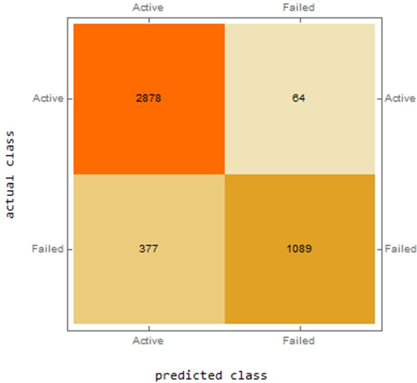
Sustainability 2020, 12, 7529                                                                       2 of 17

according to the results of an extensive study by Barboza et al. [13] and Horak et al. [14], those models
that use machine learning are, on average, 10% more accurate than traditional models created on
the basis of statistical methods. Another logical reason for the ever-increasing application of models
based on machine learning is their rapid development and improvement in many other areas [15].
These modern methods go beyond financial statements, thereby taking other elements into account.
Many studies have shown that the techniques used in the field of artificial intelligence can be a suitable
alternative for traditional statistical methods used for predicting the financial health of a company
because they do not apply past assumptions on the distribution of background data or the structure of
the relationships between the variables involved. While statistical models require the researcher to
specify the functional relationships between dependent and independent variables, non-parametric
techniques enable the data to identify the functional relationships between the variables in the model.
Within this context, the LSTM (long short-term memory) model holds a special position in that it
produces extremely good results in the area of dynamic counting, which is typical, for example,
for current electricity distribution networks, as well as for the economic environment [16]. It is for
this reason that deep learning LSTM models are used, for example, by predictive models intended for
high-frequency trading in financial markets [17] or for the prediction of future trends and the prices of
housing [18]. The application of LSTM simply produces better results than vector regression or back
propagation neural networks. Chebeir et al. [19], as well as Liu et al. [20], achieved very good results
when applying the LSTM method to the assessment and optimization of the profitability of projects
dealing with the extraction of shale gas. It is therefore surprising that there are not many bankruptcy
models based on this exceptionally progressive method.
      The objective of this study is to create a method of failure (bankruptcy) prediction that uses
artificial neural networks (hereinafter referred to as “NN”) with at least one long short-term memory
(LSTM) layer. The following research question was, therefore, formulated: Are neural networks
containing LSTM suitable for predicting potential company bankruptcy?

2. Literature Review
      Research into LSTM is very extensive. Due to its efficiency in capturing dynamic behavior and
good performance in the area of long-term dependencies, it is used for a number of applications [21].
According to [22], it can be stated that the deep architecture of a recurrent neural network (RNN) and
its variant of long short-term memory (LSTM) are more accurate than traditional statistical methods in
modelling the data of time series.
      On the other hand, they do not appear to be the best option for all areas in question. A comparative
study of LSTM, the hybrid model of convolutional neural networks, and the multi-head self-attention
approach (MHSA) by Xiao et al. [23] showed that MHSA turned out to be 6.5% better for the
field of phishing. Similarly, a specially constructed network, CSAN (Crime Situation Awareness
Network), surpassed predictive Cony-LSTM spatial temporal models in predicting crime frequency [24].
The extensive comparing of methods for logical relationships intended for fuzzy predictions of
time series, namely machine learning, LSTM, and supporting vector machines, were the basis for
evaluating supporting vector machines as more efficient than the other two [25]; according to
Liu et al. [20], the model of adaptive wavelet transform (AWTM) surpassed the LSTM model in
predicting time-frequency analysis of multi-frequency trading on stock markets. On the other hand,
the experimental results of the LSTM model, with an added layer, according to Pang et al. [26], showed a
high level of prediction accuracy for the composite stock model (56.9%, and 52.4% for individual stocks).
Other results unambiguously confirm the efficiency of LSTM, for example, in the case of predicting the
volatility of and time jumps in financial series within an analysis of 11 global stock markets [27], or in
the case of predicting the development of stock markets according to Ding and Qin [28], whose model
of associated LSTM showed a prediction accuracy of more than 95%. Chebeir et al. [19] achieved a
similar result when it came to predicting stock volatility using LSTM.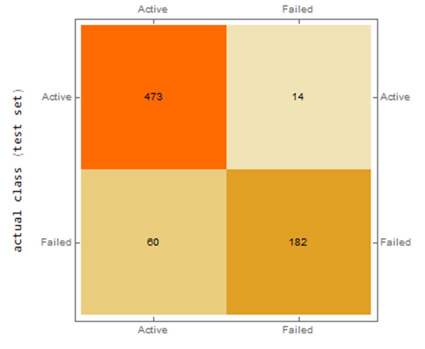
Sustainability 2020, 12, 7529                                                                        3 of 17

      The LSTM model is typically used by researchers for creating models and problem solving,
for example in gestures or speech processing. Adeel et al. [29] dealt with the combination of declared
excellent results, while Liu et al. [20] dealt with the successful classification of models working with
the self-attention mechanism and bidirectional functions (SAMF-BiLSTM). The spam filtering models
using the aforementioned method achieved a very high prediction accuracy of 99.44% [30].
      Other fields in which LSTM is often used include medicine and the energy industry. The challenge
is, for example, to combine the difficult task of predicting production from renewable resources with
consumption, where, according to Wang et al. [24], the stability of the network can be ensured by using
the LSTM module of interactive parallel prediction. Tian et al. [31] dealt with the successful prediction
of the model for optimizing the use of lithium-ion batteries in the field of energy, while Chatterjee
and Dethlefs [32] focused on the failures and anomalies in the operation of wind turbines by means of
LSTM. Hong et al. [33] pointed to the stability and robustness of this method, as verified by extensive
cross-validation and comparative analysis.
      The advantages of using LSTM in comparison with traditional model solutions are addressed in
the work of Yang et al. [34]. Zhang et al. [35] dealt with the efficiency of LSTM and FFNN (feedforward
neural networks), where LSTM was less accurate, but with a significantly longer prediction horizon.
In the same field, Yang et al. [34] proved that compared to vector modelling, LSTM showed a higher
predictive accuracy, faster response time, and stronger generalization capability. In the case of renewable
resources, Correa-Jullian et al. [36] compared the predictive methods based on standard neural networks
and LSTM. The comparison showed that LSTM models achieve the lowest RMSE (Root Mean Square
Error) error score, lowest standard deviation, and smallest relative error. LSTM’s excellent ability
to capture the time dependency of a time series was used by [10] to predict electricity consumption,
or short-term grid load. Wei et al. [37] used the combined model of singular spectrum analysis
(SSA) and LSTM to predict gas consumption. Somu and Ramamritham [38] dealt with electricity
consumption by means of another variant of ISCOA-LSTM based on a specific example. According to
the authors, it is a highly effective prediction tool. Increasing energy efficiency through a combination
of LSTM and bootstrapping was addressed in general by Zhu et al. [39].
      A predictive model of oil production applied to actual production in China achieved an almost
100% success rate [20]. The application of a highly efficient integrated convolutional neural network
(CNN) with LSTM to predict China’s future energy mix was addressed by Liu [40].
      Extensive research has shown the effectiveness of the application of LSTM for predicting the
development of prices. According to Qiao and Yang [41], the hybrid model based on wavelet
transformation (WT), sparse autoencoder (SAE), and LSTM shows a high level of accuracy with
regards to the prediction of electricity prices in the USA. Another hybrid model, WT-Adam_LSTM,
used for predicting the development of electricity prices and verified on the basis of four case studies,
was presented by Chang et al. [42].
      Due to its progressiveness, the LSTM model has been assessed and developed by a number
of authors. The assessment of the functional response of the LSTM and spiking neural network
(SNN) revealed the dominance of SNN [43]. Du et al. [44] presented an end-to-end deep learning
structure that integrates a conventional coded context vector and a time-of-attention vector for the
joint learning of time representation on the basis of the LSTM model. Wang et al. [24] dealt with the
problem of long-term dependence in sequence data due to insufficient memory capacity in LSTM cells,
solving it using an attention-aware bidirectional multi-residual recurrent neural network (ABMRNN).
Punia et al. [45] presented a new predictive method that combines LSTM and random forest (RF),
the efficiency of which is compared to other methods, such as neural networks, multiple regression,
ARIMAX (Autoregressive Integrated Moving Average with Explanatory Variable), etc.
      The effectiveness of LSTM in comparing the performances of LSTM RNN by initialized methods
of learning transmission and randomly initialized recurrent neural networks was confirmed by
Fong et al. [46]. Another variant called CTS-LSTM for the collective prediction of correlated time
series with the aim of improving the predictive accuracy of the model was presented by Wan et al. [47].
Sustainability 2020, 12, 7529 4 of 17
Bandara et al. [48] solved the problem of time series’ heterogeneity by introducing the concept of
similarity between time series. Park et al. [49] strove to improve classification performance by means of
the interaction between the model architecture factors and the dimensions of the dataset characteristics.
According to the authors, bidirectional LSTM dominated within the given aspects. Zhang et al. [35]
presented a different model of weighted auto regressive long short-term memory (WAR-LSTM), using it
to extract representative data from more than one variable. Another evolutionary model of LSTM,
focused on the transmission of shared parameters in order to increase the efficiency of prediction
in multiple time slots, was created by Liu and Liu [18]. Karim et al. [50] focused on streamlining
the solution of complex multidimensional time series classification through the transformation of
existing univariate classification models into multivariate ones, while Farzad et al. [51] focused on
activation functions, according to which the quantitative results showed that the smallest average
error is achieved by means of the Elliott activation function and modifications thereof. Another hybrid
model based on exponential smoothing combined with advanced long-term memory networks was
presented by Smyl [52].
A section in this contribution is dedicated to the potential application of LSTM to the management
of financial risks or to the prediction of company bankruptcy. Despite this, many authors continue to
work with traditional bankruptcy models, such as Altman Z-Score, Kralicek Quick Test, IN 99, IN05 [53],
hybrid models of classification and regression trees (CART), multivariate adaptive regression spline
(MARS) models [54], or evolutionary dynamics and the optimization of the strategy for certain types
of interconnected evolutionary games [55]. In other cases, for the verification of statistical bankruptcy
models, the Monte Carlo method is used [56]. Alternatively, it is possible to see the bankruptcy model
as a multivariate grey prediction problem, for which Hu [57] used genetic algorithms.
There is also the question of the verification of these methods, whereby, based on the assessment of
bankruptcy model performance (discriminant analysis, logistic regression, and multilayer perceptron
network), decision trees appear to be the most efficient [58], as well as the success rate of the bankruptcy
models, which, according to Kubenka and Myskova [59], is lower in the overall comparison of the
three methods than the researchers stated.
The application of machine learning is nothing new in the case of bankruptcy models.
For bankruptcy prediction, Zhou and Lai [60] effectively used the AdaBoost algorithm combined
with imputation, while Kim et al. [61] examined the benefits of deep learning on decision-making in
financial risk management. Liu and Liu [18] used LSTM models combined with block-chain technology
to increase financial performance and reduce risks. Koudjonou and Rout [62] dealt with the net
value of assets by means of an LSTM recurrent neural network and the comparison of single-layer,
multi-layer, unidirectional, and bidirectional networks. Bankruptcy models based on LSTM, however,
are used relatively little, despite the significant development of this method and its effectiveness,
especially in dynamically developing situations and in the case of insufficient data. The exception
is a deep learning model presented by Mai et al. [63] for predicting company bankruptcy using
text information. A comprehensive database of bankruptcy of 11,827 US companies shows that
deep-learning models provide excellent predictions; interestingly, simpler models, such as averaging
appear to be more efficient than convolutional neural networks. However, the authors themselves say
that in this case, it is the first step in using the highly progressive LSTM method within bankruptcy
models. The authors also mention the limitation of data obtained exclusively from financial statements
(MD&A–Management Discussion and Analysis) or the difficult interpretation of the results based
on the processing of unstructured data within the so-called “black box” of deep-learning models.
They therefore recommend further research by means of other deep-learning models, as well as by
means of using other tools capable of evaluating the performances of the created models, such as
H-measures or Kolmogorov–Smirnov statistics of good results.
3. Materials and Methods
The application part was organized according to the following structure, with further explanations below:Sustainability 2020, 12, 7529 5 of 17
(1) Selection and preparation of the data for the calculation.
(2) Division of the data into training and testing data sets.
(3) Creation of a bankruptcy model by means of an experiment using Mathematica Software.
(4) Generation of NN using LSTM networks and other elementwise layers.
(5) Evaluation of the performance of networks in the training and testing data sets, creation of
a confusion matrix characterizing the correct classification of companies into “active” and
“in liquidation”.
(6) Description of the best NN and discussion on the success rate of the network.
3.1. Data
The source of the data on industrial companies operating in the Czech Republic was the Albertina
database. The selected industrial companies fell under section “C” of the CZ NACE (Czech classification
of economic activities), specifically groups 10–33.
The data set included 5 consecutive marketing years (from 2014 to 2018). The data set contained
those companies able to survive potential financial distress (hereinafter also referred to as “active
companies”), as well as companies in liquidation. In total, 5500 companies were included. Data rows
(one company and one year representing one data row) with nonsensical data or with a large amount
of information missing were excluded.
For the purpose of the analysis, selected items from financial statements were used, specifically the
balance sheet and profit and loss statement.
For this analysis, only some of the items were used:
• AKTIVACELK—total assets, i.e., the result of economic activities carried out in the past. This represents
the future economic profit of the company.
• STALAA—fixed assets, i.e., long-term, fixed, non-current items, including property components,
used for company activities over the long run (for more than one year) and consumed over time.
• OBEZNAA—current assets characterized by the operating cycle, i.e., they are in constant motion
and change form. These include money, materials, semi-finished products, unfinished products,
finished products, and receivables from customers.
• KP—short-term receivables with a maturity of less than 1 year, representing the right of the
creditor to demand the fulfilment of a certain obligation from the other party. The receivable
ceases to exist upon the fulfilment of the obligation.
• VLASTNIJM—equity, i.e., the company’s resources for financing assets in order to create capital.
This primarily concerns the contributions of the founders (owners or partners) to the basic capital
of the company and those components arising from the company’s activities.
• CIZIZDROJE—borrowed capital, i.e., company debts that have to be repaid within a specified
period of time. This represents the company’s liabilities towards other entities.
• KZ—short-term liabilities, i.e., due within 1 year. Together with equity, they ensure the financing
of the day-to-day activities of the company. These primarily include bank loans, liabilities to
employees and institutions, debts to suppliers or taxes due.
• V—performance, i.e., the results of company activities which are characterized by the main activity
of the company—production. This includes the goods and services used for satisfying demands.
• SLUZBY—services, i.e., those activities intended to meet human needs or the needs of a company
by means of their execution.
• PRIDHODN—added value, i.e., trademarking, sales, changes in inventory through own
activities, or activation reduced by power consumption. This includes both company margin
and performance.
• ON—personnel costs, i.e., gross salaries and the employer’s compulsory social and health
insurance contributions for each employee.Sustainability 2020, 12, 7529 6 of 17
• PROVHOSP—operating results, i.e., the outcomes and products that reflect the ability of a
company to transform production factors.
• NU—interest payable, i.e., the price of borrowed capital.
• HOSPVZUO—economic result for an accounting period, i.e., from operational, financial,
and extraordinary activities.
• STAV—target situation, i.e., classification as “active” for companies able to survive potential
financial distress, and “in liquidation” for companies that will go bankrupt.
Absolute indicators characterize a company from several perspectives. They evaluate the structure
of the company´s capital, the price of capital, its technological level (by means of added value),
the ability to perform its main activity (that is, to transform production factors into products), and to
achieve one of the main goals of its existence (to generate profit). A number of authors (e.g., Altman)
have used ratios to create a method for predicting market failure. In such cases, two possible reasons
can be identified. Firstly, they anticipated the economic interpretation of their models’ segments,
therefore giving their models certain economic rationality. Secondly, they simplified the computing
power requirements. This specifically concerns the reduction of future model data. In the model,
the NN acts like a black box if the identification of the calculated result is difficult. It is, therefore,
not necessary to follow the economic interpretation of each bond of neurons and the propagated signal
because the bond as such is insignificant. In addition, it is subsequently not necessary to limit the
number of variables. Hardware computing power is able to process a large amount of data during
its creation. For the application of the NN generated, a fraction of the computing power is necessary
compared to the preparation stage of the NN.
After the aforementioned modifications (removal of nonsensical data, etc.), the data were divided
into two datasets: a training and a testing dataset. The training dataset was used to train the neural
structure, while the testing dataset was used for the validation of the result. The statistical characteristics
of the individual items in the training and testing datasets are presented in Table 1.
Table 1. Statistical characteristics of the datasets.
Training Testing
Item
Minimum Maximum Mean Standard Deviation Minimum Maximum Mean Standard Deviation
Total Assets 0 6,963,568 101,794.3 421,183.6 0 62,924,684 193,629.3 2,402,017
Fixed Assets −19,065 4,558,816 49,269.92 251,519.4 0 30,832,576 90,484.69 1,204,674
Current Assets 0 2,391,855 51,801.29 182,982.9 0 32,066,562 102,624.7 1,222,082
Short Term Receivables −127 1,947,964 24,162.22 106,237.4 0 27,683,668 65,334.36 1,039,648
Equity −9662 1,923,390 50,993.7 186,972.2 −206,208 53,318,744 131,475.4 2,004,015
Borrowed Capital 0 5,024,089 50,269.76 256,551.2 −21 9,605,513 61,351.15 469,600.1
Short Term Liabilities 0 4,906,382 31,905.76 204,347.7 −96 7,970,386 41,665.4 366,137.2
Performance −40 4,180,449 97,214.31 335,148.6 −246 33,887,311 142,956.2 1,342,696
Services 0 569,454 14,468.57 48,754.07 0 3,038,338 19,348.75 133,230.2
Added Value −7788 824,345 26,734.39 76,957.12 −20,284 3,457,583 30,516.86 167,441.7
Personnel Costs 0 463,685 17,940.92 46,808.62 −60 2,665,233 19,125.81 111,284.5
Operating Result −150,310 852,991 7316.556 44,552.34 −847,530 914,063 4213.27 63,193.46
Interest Payable 0 187,218 744.4554 7525.506 0 52,798 494.3265 2912.81
Economic Result for
−245,135 700,092 6354.041 43,196.58 −645,493 673,179 5049.786 53,302.32
Accounting Period (+/−)
Source: Own processing according to Albertina database.
3.2. Methods
The bankruptcy model was created using an artificial deep learning neural network. As indicated
by the research carried out and the objective of the contribution, at least one layer of LSTM was used for
the creation of the NN. For the solution of the problem, Wolfram’s Mathematica software (version 13)
was used.
The specific NN structure was determined by an experiment. The individual layers consisted of
the following components:Sustainability 2020, 12, 7529 7 of 17
The input layer: 1 × 14 matrix. The matrix consisted of one row that included 14 input continuous
variables (AKTIVACELK, STALAA, OBEZNAA, KP, VLASTNIJM, CIZIZDROJE, KZ, V, SLUZBY,
PRIDHODN, ON, PROVHOSP, NU, HOSPVZUO).
1st hidden layer: LSTM layer. The output was a 1 × n matrix, whereby the number of matrix
elements was part of the experiment. The size of the matrix influenced the predictive ability of the
model. A low number of matrix elements could generate a result with a higher level of inaccuracy,
whereas a high number of elements could make the model too complex and overfitted (it shows
excellent performance parameters for the training dataset, but is totally incapable of generating a
proper classification for the testing dataset). The number of matrix elements was at the interval between
5 and 2000 elements.
2nd hidden layer: elementwise layer. The objective was to add a certain degree of non-linearity to
the NN. A partial experiment was carried out on the basis of which the suitability of the following
functions was tested:
• Hyperbolic tangent (Tanh),
• Sinus (Sin),
• Ramp (referred to as ReLU),
• Logistic function (logistic sigmoid).
3rd hidden layer: elementwise layer. The objective was to add a certain degree of non-linearity to
the NN. As this was the second elementwise layer, the non-linearity was stronger. Also in this case,
a partial experiment was carried out. The suitability of the following functions was tested accordingly:
• Hyperbolic tangent (Tanh),
• Sinus (Sin),
• Ramp (referred to as ReLU),
• Logistic function (logistic sigmoid).
4th hidden layer of neurons: LSTM layer. The output was a 1 × 2 matrix. The size of the matrix
was determined by the number of possible results—predicting either “active” or “in liquidation”.
Output layer: two neurons representing a vector with two elements. The vector was subsequently
decoded as “active company” or “company in liquidation”.
3.3. Long-Short Term Memory Layer
LSTM is considered to be a specific type of recurrent NN consisting of several components. It is
possible to identify the elementwise layer with the logistic sigmoid function and hyperbolic tangent,
linear layer, concatenate layer, copy layer, and the transfer of the data in the form of vectors.
The basic LSTM processes are defined as input gate, output gate, forget gate, and memory gate.
The state of the cell is defined as follows:
ct = ft ∗ ct−1 + it ∗ mt , (1)
where:
ct : new state of the variable;
ft : forget gate;
ct−1 : original state of the variable;
it : input gate;
mt : memory gate.
The input gate is defined as follows:
it = σ[Wix xt + Wis st−1 + bi ], (2)Sustainability 2020, 12, 7529 8 of 17
where:
σ: logistic sigmoid;
Wix : input weight in input gate, matrix n × k;
xt : input variable, n × k matrix;
Wis : weight in input gate, n × n matrix;
st−1 : previous state;
bi bias: vector size n.
The state is determined by the following formula:
st = ot ∗ Tanh[ct ], (3)
where:
st : state of the variable;
ot : output gate;
Tanh: hyperbolic tangent.
Output gate is represented by the formula below:
ot = σ[Wax xt + Was st−1 + bo ], (4)
where:
Wax : input weight in output gate, n × k matrix;
Was : weight in output gate, n × n matrix;
bo bias: vector size n.
Forget gate is an important innovation of LSTM:
h i
ft = σ W f x xt + W f s st−1 + b f , (5)
where:
Wfx : determines the forget gate input weigh, n × k matrix;
Wfs : weight in forget gate, n × n matrix;
bf : vector size n.
The last main process to determine is memory gate:
mt = Tanh[Wmx xt + Wms st−1 + bm ] (6)
where:
Wmx : input weight in memory gate, n × k matrix;
Wms : weight in memory gate, n × n matrix;
Bm : vector size n.
3.4. Elementwise Layer
The elementwise layer is a single layer of neurons that takes n inputs from the previous layer.
It adds non-linearity in the calculation and transfers n inputs to another layer of the NN.
As part of the research presented in this contribution, non-linearity was added in the form of
testing in the 2nd and 3rd hidden layers using the following functions:
1. Hyperbolic tangent (Tanh):
ex − e−x
f (x) = tanhx = . (7)
ex + e−xSustainability 2020, 12, 7529 9 of 17
2. Sinus (Sin):
f (x) = Sin(x). (8)
3. Ramp (referred to as ReLU):
R(x) : R → R0+ . (9)
4. Logistic function (logistic sigmoid):
1
f (x) = . (10)
1 + e−x
3.5. Evaluation of Network Performance
Within the experiment mentioned above, 1000 neural networks were generated, with differing
sizes of the vector from the first LSTM layer and the activation function of the 2nd and 3rd layer of NN.
The evaluation of the networks was based on:
1. The performance of the individual networks in the training and testing datasets.
2. The confusion matrix characterizing the correct classification of companies into “active” and “in
liquidation”. The confusion matrix was created for both the training and testing datasets.
The best NN is subsequently described in detail in terms of its characteristics. However, if the
network showed signs of overfitting, the second most successful network (in terms of its parameters)
was then used.
4. Results
Within the experiment, a total of 1000 NNs were generated and their performance in the training
and testing datasets compared. The highest possible performance was sought in all datasets and
all parameters (“active”, “in liquidation”) and, at the same time, similar in the training and testing
datasets. Table 2 shows the neural networks with the best performance parameters.
Table 2. NN with best performance parameters.
Training Performance Test Performance
ID NN Neural Network
Active Failed Total Active Failed Total
1. 14-940-Tanh-Tanh-2-1 0.978246 0.742838 0.899955 0.971253 0.752066 0.898491
2. 14-1970-Ramp-Tanh-2-1 0.978586 0.722374 0.893376 0.967199 0.750331 0.899863
3. 14-1980-Ramp-Sin-2-1 0.976547 0.718963 0.89088 0.973306 0.747934 0.898491
4. 14-1990-Sin-Sin-2-1 0.973148 0.736016 0.894283 0.975359 0.747934 0.899863
5. 14-1010-Tanh-Sin-2-1 0.980625 0.734652 0.89882 0.967146 0.772727 0.902606
Source: Authors.
The network structure was as indicated above. The value 14 indicates the number of neurons in
the input layer. It is a 1 × n matrix, i.e., a vector of variables. The second value in the NN structure
indicates the number of elements of the vector (1 × n matrix) of the new state of the variables from the
LSTM layer, i.e., the output of the first hidden layer of the NN. What follows in succession are the
activation function of the second hidden layer of neurons, the activation function of the third hidden
layer of neurons, the output of the second LSTM layer, i.e., a vector (or 1 × 2 matrix), and the final
state, i.e., whether the company was “active” or “in liquidation”. The training performance provided
information on the accuracy of the classification determined under the training dataset, and the testingSustainability 2020, 12, 7529 10 of 17
performance provided information on the accuracy of the classification determined under the testing
(validation) dataset.
A neural structure was sought of which the performance was as close to 1 as possible in all datasets.
It is important for the results that the performance value is, ideally, the same for all datasets and groups.
On the basis of this evaluation, the network identified as ID 1 appears to be the best. Its overall
performance was 0.978 for the training dataset and 0.971 for the testing dataset. However, there is a big
problem with regards to predicting companies that will go bankrupt. This is due to the fact that the
Sustainability
decision 2020, 12,
to enter x FOR
into PEER REVIEW
liquidation is often not based on the management or the owners’ rational decision 10 of 18
on the economic and financial sustainability of a company. Under such circumstances, it may happen
when
that predictingthat
a company failure,
couldthebeevaluator or theceases
able to operate modelitsmust remove
activities a large Obviously,
anyway. amount of noise. In the case
when predicting
of NN ID
failure, the1,evaluator
the performance with must
or the model regards to predicting
remove failure was
a large amount almost
of noise. In 0.743 for of
the case theNNtraining
ID 1,
dataset and 0.752 for the testing dataset (i.e., even more than for the training
the performance with regards to predicting failure was almost 0.743 for the training dataset and 0.752dataset). The NN
therefore suffered from overfitting, showing excellent performance parameters,
for the testing dataset (i.e., even more than for the training dataset). The NN therefore suffered from but zero
applicability,
overfitting, as stated
showing above.performance
excellent As a result, other successful
parameters, but zeronetworks wereasretained
applicability, and other
stated above. As a
successful NNs analyzed.
result, other successful networks were retained and other successful NNs analyzed.
Figure 11 shows
Figure shows the the structure
structureof ofNN
NNIDID1.1.
Figure 1. Structure of neural network (NN) ID 1 (14-940-Tanh-Tanh-2-1).
(14-940-Tanh-Tanh-2-1).
The
The figure
figureshows
shows14 14neurons
neuronsin inthe
theinput
inputlayer. wasaa11×× 14
layer.ItItwas 14 matrix
matrix that
that characterizes
characterizes the
the input
input
data of a company (asset structure, capital structure, price of capital, technological
data of a company (asset structure, capital structure, price of capital, technological level, the ability level, the ability
to
to carry
carry outout its
its own
own activities
activities and
and make
make profits).
profits). There
There was was also
also aa LSTM
LSTM layer,
layer, the
the output
output ofof which
which
was a 1 × 940 matrix (or a vector with 940 elements). To the individual matrix
was a 1 × 940 matrix (or a vector with 940 elements). To the individual matrix elements, non-linearity elements, non-linearity
was
was added
added inin the
the subsequent
subsequent two two layers.
layers. In In both
both elementwise
elementwise layers,
layers, it it concerned
concerned aa function
function ofof the
the
hyperbolic tangent. The following layer was the LSTM layer, the output
hyperbolic tangent. The following layer was the LSTM layer, the output of which was a 1 × 2 matrix of which was a 1 × 2 matrix
(or
(or vector
vectorwith
with22elements),
elements),fromfromwhich
whichthe theresult
resultwas
was derived,
derived,i.e., thethe
i.e., company
company was either
was “active”
either “active” or
“in liquidation”.
or “in liquidation”. In terms of the
In terms of internal
the internalfunctioning of theofwhole
functioning NN, both
the whole NN, LSTM layerslayers
both LSTM appear to be
appear
of interest. The elementwise layer only represented a certain mechanical
to be of interest. The elementwise layer only represented a certain mechanical element that changed element that changed the
distribution
the distributionof the signal
of the in another
signal in another NN NN layer.
layer.The
Theinner
inner structure
structureofofthe thefirst
firstLSTM
LSTMlayer
layer(the
(the first
first
inner layer of the NN) is presented
inner layer of the NN) is presented in Table 3. in Table 3.
The structure of the LSTM layer shows the distribution of the information in the layer, mainly the
relationshipTable between thestructure
3. Inner input data of theand the
first longoutput vector
short-term with 940
memory elements.
(LSTM) layer ofThe
NN structure
ID 1. of the
second LSTM layer (the fourth hidden layer of the NN) is similarly presented in Table 4.
If the inserted non-linearity Fieldwere left aside Type and the of Output
whole processSize of of Output
data transformation was
Input gate input weights
simplified, it turned out that 14 data on a company entered into the NN. The matrix 940 × 14 data were analyzed
Input gate state weights matrix
and their combinations expressed as 940 values, which were subsequently analyzed (more precisely, 940 × 940
their combinationsInput were gate biasesand reduced to twovector
analyzed) target values expressing 940 the probability of the
company being classified as “active” or “in liquidation”. At the end of the ×NN,
Output gate input weights matrix 940 14 there was a decoder
Output gate state weights
that determined the assumed state of the company on the basis of probability.matrix 940 × 940
Output gate biases vector 940
• The trained NN in the
Forget WLNet
gate inputformat
weights is availablematrix
from: https://ftp.vstecb.cz
940 × 14
• The training dataset
Forget in xlsx
gate format
state is available from:
weights https://ftp.vstecb.cz
matrix 940 × 940
• The testing datasetForgetingate
xlsxbiases
format is available from: vector
https://ftp.vstecb.cz 940
Memory gate input weights matrix 940 × 14
Memory gate state weights matrix 940 × 940
Memory gate biases vector 940
Source: Authors.Sustainability 2020, 12, 7529 11 of 17
Table 3. Inner structure of the first long short-term memory (LSTM) layer of NN ID 1.
Field Type of Output Size of Output
Input gate input weights matrix 940 × 14
Input gate state weights matrix 940 × 940
Input gate biases vector 940
Output gate input weights matrix 940 × 14
Output gate state weights matrix 940 × 940
Output gate biases vector 940
Forget gate input weights matrix 940 × 14
Forget gate state weights matrix 940 × 940
Forget gate biases vector 940
Memory gate input weights matrix 940 × 14
Memory gate state weights matrix 940 × 940
Memory gate biases vector 940
Source: Authors.
Table 4. Inner structure of the second LSTM layer of NN ID 1.
Field Type of Output Size of Output
Input gate input weights matrix 2 × 940
Input gate state weights matrix 2×2
Input gate biases vector 2
Output gate input weights matrix 2 × 940
Output gate state weights matrix 2×2
Output gate biases vector 2
Forget gate input weights matrix 2 × 940
Forget gate state weights matrix 2×2
Forget gate biases vector 2
Memory gate input weights matrix 2 × 940
Memory gate state weights matrix 2×2
Memory gate biases vector 2
Source: Authors.
5. Discussion
A NN was obtained that, at first sight, is able to predict, with a high probability, the future
development of a company operating in the manufacturing sector in the Czech Republic. The results
described clearly show the structure of the network and the method of data processing in the network.
Both the NN and the background data are available for calculation for the validation of the results and
for practical application. However, it is necessary to consider the practical or theoretical benefits of the
NN obtained and its applicability in practice.
The theoretical benefit of this contribution consists in the possibility to apply LSTM NN as a
tool for predicting bankruptcy. It was verified and proved that this type of recurrent NN is able to
process and analyze data on a company, as well as produce a result. In terms of the theoretical benefit,
instead of the results of the model, it is necessary to procedurally monitor (mathematically in this case)
whether it is possible to process the data and obtain a meaningful result. The NN structure could be
further processed and adapted to the required outputs. It is also possible to train the NN (and the
partial weights of the NN) so that it is possible to obtain the correct results in the required structure.
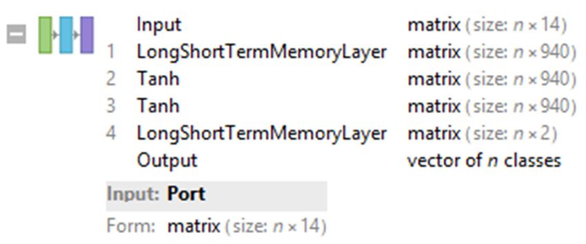
The practical application of the NN with the LSTM layers was confirmed mainly by the confusion
matrix for the training and testing datasets. Figure 2 shows the confusion matrix for the training dataset.Sustainability 2020, 12, 7529 12 of 17
Sustainability 2020, 12, x FOR PEER REVIEW 12 of 18
Sustainability 2020, 12, x FOR PEER REVIEW 12 of 18
Confusion matrix
Figure 2. Confusion matrix for
for the
the training
training dataset.
dataset.
The confusion matrix for the training dataset shows that the NN appears to be very successful in
predicting the ability to overcome potential financial distress. In 2878 cases, the result was predicted
correctly, with only 64 errors. For the same dataset, it predicted bankruptcy for 1089 companies,
with 377 errors. This is the aforementioned noise arising from the fact that a number of companies
cease their activities without being forced to do so by their financial and economic results. Despite this,
this represents an excellent Figure
result. 2.Figure 3 presents
Confusion matrix the results
for the for the
training testing dataset.
dataset.
Figure 3. Confusion matrix for the testing dataset.
The second confusion matrix also produced excellent results. Of the 487 active companies, the
NN was able to identify 473 companies able to survive potential financial distress; of the 262
companies identified as going bankrupt, the NN identified 182.
By default, the successful prediction rate was higher than 50% in those situations where it was
not a coincidence. In the case of NN ID 1, the overall successful prediction rate was higher than 97%
Figure 3. Confusion matrix for the testing dataset.
for all companies and 75% for Figure
those 3. going
Confusion matrix for
bankrupt. the therefore
It can testing dataset.
be concluded that the NN with
the LSTM layer (NN
The second ID 1 in
confusion particular)
matrix is applicable
also produced in practice.
excellent results. It Ofisthe
possible to compare
487 active companies, the the
results
NN
with The
othersecond confusion
studies. For matrix
example, also produced
Mihalovic [64] excellent
dealt with results.
the Of the
application
was able to identify 473 companies able to survive potential financial distress; of the 262 companies
487 of active
the companies,
original Altman the
NN was
Index able
Z-Score.
identified
to identify
The
as going authors 473
bankrupt, focusedcompanies
the NNonidentified
able182.
the financial to survive
statements potential financial
of 373 Greek distress;inofthe
companies the 262
years
companies
1999–2006. identified
The results as going bankrupt,
of their studies the
indicated NN identified
thathigher
the success 182. rate of
By default, the successful prediction rate was than 50% in the model
those was 52%
situations wheretwoityears
was
beforeBybankruptcy
default, theand successful
66% one prediction
year before rate was higher
bankruptcy. It than 50%
should alsoinbethose situations
mentioned thatwhere
the it was
authors
not a coincidence. In the case of NN ID 1, the overall successful prediction rate was higher than 97%
not a coincidence.
used In the ofcase of NN IDindex;
1, the overall successful prediction rate
in was higher thanyears 97%
for allthe market value
companies and 75% equity
for thosein the
going the results,
bankrupt. It cantherefore,
thereforediffered
be concluded the that
individual
the NN with
for
and all companies
also according and
to ID 75% for
the1actual those going bankrupt.
situationisofapplicable
the financial It can therefore
markets.ItThe be concluded
issue of predictivethat the NN with
the LSTM layer (NN in particular) in practice. is possible to comparemodels was
the results
the LSTM
also layerby
addressed (NN ID 1 in particular)
Mihalovic [64], who is applicable
focused on in practice.
predictive It is possible
bankruptcy to compare
models for a the results
total of 236
with other studies. For example, Mihalovic [64] dealt with the application of the original Altman
with
Slovak other studies.
companies. For example, Mihalovic [64] dealt with the application of the original Altman
Index Z-Score. TheIn the study,
authors focused the on
author primarilystatements
the financial comparedofthe 373 overall
Greekpredictive
companiesperformance
in the years
Index
of two Z-Score.
models, The
the authors
first based focused
on on the financial
discriminant statements
analysis and theofsecond
373 Greekon companies
logistic in the years
regression. The
1999–2006. The results of their studies indicated that the success rate of the model was 52% two years
1999–2006.
results The results
of the research of their studies indicated that the success rate of the model was 52% two years
before bankruptcy and showed
66% one that yearthe model
before based onItthe
bankruptcy. logit also
should function providedthat
be mentioned moretheaccurate
authors
before bankruptcy
results, and that the andmost66%important
one year before
factorsbankruptcy.
that prevent It should also of
the failure be amentioned
company that are the authors
short-term
used the market value of equity in the index; the results, therefore, differed
assets, short-term liabilities, net income, and total assets. Lin [65] examined the predictive power in the individual years
of
and also according to the actual situation of the financial markets. The issue of predictive models was
also addressed by Mihalovic [64], who focused on predictive bankruptcy models for a total of 236
Slovak companies. In the study, the author primarily compared the overall predictive performance
of two models, the first based on discriminant analysis and the second on logistic regression. TheSustainability 2020, 12, 7529 13 of 17
used the market value of equity in the index; the results, therefore, differed in the individual years and
also according to the actual situation of the financial markets. The issue of predictive models was also
addressed by Mihalovic [64], who focused on predictive bankruptcy models for a total of 236 Slovak
companies. In the study, the author primarily compared the overall predictive performance of two
models, the first based on discriminant analysis and the second on logistic regression. The results
of the research showed that the model based on the logit function provided more accurate results,
and that the most important factors that prevent the failure of a company are short-term assets,
short-term liabilities, net income, and total assets. Lin [65] examined the predictive power of the
four most commonly used models of financial distress. On the basis of his study, he created reliable
predictive models related to the bankruptcy of public industrial companies in Taiwan, specifically, logit,
probit, and artificial neural network models. The author concluded that the aforementioned models are
able to generalize and show higher predictive accuracy. It also showed that the probit model has the
most stable and best performance. Unvan and Tatlidil [66] dealt with the comparison of models that
could be applied in bank investigations and the supervisory process for detecting banks with serious
problems. The dataset consisted of 70 Turkish banks and included information on their financial
situation, as well as data on their capital adequacy, liquidity, asset quality, cost and return structure,
and profitability. Using variable methods of choosing financial data, the most important financial
characteristics were determined and subsequently used as independent variables to create probit
and logit models. Finally, these models were compared with the selected best models with the best
predictive power. Jifi [67] evaluated the accuracy and power of conventional credibility and bankruptcy
models. For the purposes of the evaluation, companies operating in the construction field in the Czech
Republic, which went bankrupt within a period of 5 years, were selected. For each of the companies,
the evaluation was carried out by means of the following models: Kralicek Quick test, the plausibility
index, Rudolf Doucha’s balance analysis, Grünwald’s index, D-score, Aspect Global Rating of the
Altman model, Taffler’s model, Springate score, the Zmijewski X-Score model, and all variants of the
IN index. The overall evaluation was subsequently based on the success rate of the individual models.
The research results revealed that the most successful model for predicting bankruptcy is the Aspect
Global Rating with a success rate of 99%, followed by Zmijewski (95%). Given the specific features of
the recent financial crisis, Iturriaga and Sanz [68] created a model of NN to study the bankruptcy of
American banks. Their research combined multilayer perceptrons and self-organizing maps, therefore
providing a tool that displays the probability of failure up to three years in advance. On the basis
of the failures of US banks between May 2012 and December 2013, the authors created a model for
detecting failure and a tool for assessing banking risk in the short, medium, and long term. This model
was able to detect 96.15% of failures, therefore overcoming the traditional models of bankruptcy
prediction. Bateni and Asghari [69] predicted bankruptcy using techniques for predicting logit and
genetic algorithms. The study compared the performance of predictive models on the basis of the data
obtained from 174 bankrupt and non-bankrupt Iranian companies listed on the Tehran Stock Exchange
in the years 2006–2014. The research results showed that the genetic model in training and testing
samples achieved 95% and 93.5% accuracy, respectively, while the logit model achieved only 77% and
75% accuracy, respectively. The results show that these two models are able to predict bankruptcy,
while, in this respect, the model of genetic algorithms is more accurate than the logit model.
The ability to predict the future state of companies creates the potential to apply NN in practice.
However, there is a problem with the complex structure of the NN. It cannot be recalculated or
programmed in a different environment than Wolfram’s Mathematica software or in the form of C++
code or Java. Managers or financial managers do not have such knowledge. Even this contribution
only presents selected characteristics of the NN ID 1 and is not able to capture the whole structure
of the best NN. Taking into account, for example, the Altman Z-Score [70] and Zeta [71] models,
their advantage is in the fact that users are able to implement them themselves with minimum
requirements in terms of their knowledge of mathematics or deep knowledge of the issue of company
financial management. The problem is how to present the NN to the public so that it is applicableSustainability 2020, 12, 7529 14 of 17
even for a layman. The solution could be the implementation of the NN in an application for company
evaluation or the creation of a user-friendly interface. Both alternatives require the use of information
and communication technologies, and the users’ remote access to the NN.
It is, therefore, possible to formulate the answers to the research question about whether neural
networks containing LSTM are suitable for predicting the potential bankruptcy of a company.
Yes, neural networks containing a LSTM layer are suitable for predicting the potential bankruptcy
of a company. However, there is a problem if a layman wants to use the model. For laymen, the model
will only be applicable when it is accessible through a user-friendly interface.
6. Conclusions
It is clear that NNs are currently not only able to solve a number of tasks in the economic
sphere but are also more efficient in doing so than models created using conventional statistical
methods (e.g., using logistic regression). So far, there have been a number of concepts of NN
imitating the actual biological neural structure. Researchers have already moved on from basic NN
(e.g., multilayer perceptron NN or generalized regression NN, deep learning). Deep learning networks
have the potential to solve relatively complex tasks. This is also evident from the NN ID 1 that arose out
of the aforementioned research into company failure. This NN is able to predict the future development
of a company operating in the manufacturing sector in the Czech Republic. The NN ID 1 is flexible and
can be trained on different datasets for different environments (temporally, spatially, and materially
different). The objective of the research and this contribution has therefore been achieved.
However, the result was limited by the transferability of the NN and its application for professional
and lay public. Although the result of the NN application was clear and easy to interpret, the model is
not easily graspable for professionals and laymen with a poor command of ICT, as it is too complex.
From the above, further direction of research follows. The factual side can “only” be adjusted in
order to improve the network’s performance. However, the formal side, in other words, the simple
presentation of the model and its easy applicability, must be solved.
The limitations of the application of the proposed method for predicting market failure lie mainly
in the requirement for available data on a company. The problem with this is the difference in
accounting methods applied in specific countries to individual items. This shortcoming could either be
solved by preparing the data prior to processing or through NN overfitting. A significant limitation
is the difficult work with the created NN. It can only be used by laymen if the network runs in the
background and the user has a user-friendly environment, for example, in the form of a thin client
operated by means of a web browser. The resulting NN will be more easily accessible to an expert who
has a command of NNs, and especially of the Mathematica software environment, or who is able to
program in cascading languages. Nevertheless, even this shortcoming can be solved, as most small-
and medium-sized companies and all large companies use websites and programmers who can apply
the method (once or by means of a simple thin client), since the NN representing the method is being
freely distributed by the authors—the link is given in Section 4: Results.
Author Contributions: Conceptualization, M.V. and J.V.; methodology, M.V.; software, J.V. and P.S.; validation,
J.V. and P.S.; formal analysis, P.S.; investigation, M.V. and J.V.; resources, P.S.; data curation, J.V.; writing—original
draft preparation, M.V.; writing—review and editing, J.V. and P.S.; visualization, J.V.; supervision, M.V.;
project administration, M.V. and P.S. All authors have read and agreed to the published version of the manuscript.
Funding: This research received no external funding.
Conflicts of Interest: The authors declare no conflict of interest.
References
1. Tang, Y.; Ji, J.; Zhu, Y.; Gao, S.; Tang, Z.; Todo, Y. A differential evolution-oriented pruning neural network
model for bankruptcy prediction. Complexity 2019, 2019, 1–21. [CrossRef]
2. Kliestik, T.; Misankova, M.; Valaskova, K.; Svabova, L. Bankruptcy prevention: New effort to reflect on legal
and social changes. Sci. Eng. Ethics 2018, 24, 791–803. [CrossRef] [PubMed]Sustainability 2020, 12, 7529 15 of 17
3. Kliestik, T.; Vrbka, J.; Rowland, Z. Bankruptcy prediction in Visegrad group countries using multiple
discriminant analysis. Equilib. Q. J. Econ. Econ. Policy 2018, 13, 569–593. [CrossRef]
4. Horak, J.; Krulicky, T. Comparison of exponential time series alignment and time series alignment using
artificial neural networks by example of prediction of future development of stock prices of a specific company.
In Proceedings of the SHS Web of Conferences: Innovative Economic Symposium 2018—Milestones and
Trends of World Economy (IES2018), Beijing, China, 8–9 November 2018. [CrossRef]
5. Antunes, F.; Ribeiro, B.; Pereira, F. Probabilistic modeling and visualization for bankruptcy prediction.
Appl. Soft Comput. 2017, 60, 831–843. [CrossRef]
6. Machova, V.; Marecek, J. Estimation of the development of Czech Koruna to Chinese Yuan exchange rate
using artificial neural networks. In Proceedings of the SHS Web of Conferences: Innovative Economic
Symposium 2018—Milestones and Trends of World Economy (IES2018), Beijing, China, 8–9 November 2018.
[CrossRef]
7. Gavurova, B.; Packova, M.; Misankova, M.; Smrcka, L. Predictive potential and risks of selected bankruptcy
prediction models in the Slovak company environment. J. Bus. Econ. Manag. 2017, 18, 1156–1173. [CrossRef]
8. Nakajima, M. Assessing bankruptcy reform in a model with temptation and equilibrium default. J. Public
Econ. 2017, 145, 42–64. [CrossRef]
9. Horak, J.; Machova, V. Comparison of neural networks and regression time series on forecasting development
of US imports from the PRC. Littera Scr. 2019, 12, 22–36.
10. Alaminos, D.; Del Castillo, A.; Fernández, M.A.; Ponti, G. A global model for bankruptcy prediction.
PLoS ONE 2016, 11. [CrossRef]
11. Alaka, H.A.; Oyedele, L.O.; Owolabi, H.A.; Kumar, V.; Ajayi, S.O.; Akinade, O.O.; Bilal, M. Systematic
review of bankruptcy prediction models: Towards a framework for tool selection. Expert Syst. Appl. 2018, 94,
164–184. [CrossRef]
12. Eysenck, G.; Kovalova, E.; Machova, V.; Konecny, V. Big data analytics processes in industrial internet
of things systems: Sensing and computing technologies, machine learning techniques, and autonomous
decision-making algorithms. J. Self-Gov. Manag. Econ. 2019, 7, 28–34. [CrossRef]
13. Barboza, F.; Kimura, H.; Altman, E. Machine learning models and bankruptcy prediction. Expert Syst. Appl.
2017, 83, 405–417. [CrossRef]
14. Horák, J.; Vrbka, J.; Šuleř, P. Support vector machine methods and artificial neural networks used for the
development of bankruptcy prediction models and their comparison. J. Risk Financ. Manag. 2020, 13, 3390.
[CrossRef]
15. Vrbka, J.; Rowland, Z. Using artificial intelligence in company management. In Digital Age: Chances, Challenges
and Future, 1st ed.; Lecture Notes in Networks and Systems; Ashmarina, S.I., Vochozka, M., Mantulenko, V.V.,
Eds.; Springer: Cham, Switzerland, 2020; pp. 422–429. [CrossRef]
16. Zheng, C.; Wang, S.; Liu, Y.; Liu, C.; Xie, W.; Fang, C.; Liu, S. A novel equivalent model of active distribution
networks based on LSTM. IEEE Trans. Neural Netw. Learn. Syst. 2019, 30, 2611–2624. [CrossRef] [PubMed]
17. Rundo, F. Deep LSTM with reinforcement learning layer for financial trend prediction in FX high frequency
trading systems. Appl. Sci. 2019, 9, 4460. [CrossRef]
18. Liu, R.; Liu, L. Predicting housing price in China based on long short-term memory incorporating modified
genetic algorithm. Soft Comput. 2019, 23, 11829–11838. [CrossRef]
19. Chebeir, J.; Asala, H.; Manee, V.; Gupta, I.; Romagnoli, J.A. Data driven techno-economic framework for the
development of shale gas resources. J. Nat. Gas Sci. Eng. 2019, 72, 103007. [CrossRef]
20. Liu, W.; Liu, W.D.; Gu, J. Forecasting oil production using ensemble empirical model decomposition based
Long Short-Term Memory neural network. J. Pet. Sci. Eng. 2020, 189, 107013. [CrossRef]
21. Karevan, Z.; Suykens, J.A.K. Transductive LSTM for time-series prediction: An application to weather
forecasting. Neural Netw. 2020, 125, 1–9. [CrossRef]
22. Sagheer, A.; Kotb, M. Unsupervised pre-training of a deep LSTM-based stacked autoencoder for multivariate
time series forecasting problems. Sci. Rep. 2019, 9, 19038. [CrossRef]
23. Xiao, X.; Zhang, D.; Hu, G.; Jiang, Y.; Xia, S. A Convolutional neural network and multi-head self-attention
combined approach for detecting phishing websites. Neural Netw. 2020, 125, 303–312. [CrossRef]
24. Wang, B.; Zhang, L.; Ma, H.; Wang, H.; Wan, S. Parallel LSTM-Based regional integrated energy system
multienergy source-load information interactive energy prediction. Complexity 2019, 2019, 1–13. [CrossRef]You can also read