A scenario modeling pipeline for COVID 19 emergency planning - Nature
←
→
Page content transcription
If your browser does not render page correctly, please read the page content below
www.nature.com/scientificreports
OPEN A scenario modeling pipeline
for COVID‑19 emergency planning
Joseph C. Lemaitre1,8, Kyra H. Grantz2,8, Joshua Kaminsky2,8, Hannah R. Meredith2,8,
Shaun A. Truelove3,4,8, Stephen A. Lauer2, Lindsay T. Keegan5, Sam Shah6, Josh Wills6,
Kathryn Kaminsky7, Javier Perez‑Saez2, Justin Lessler2 & Elizabeth C. Lee2*
Coronavirus disease 2019 (COVID-19) has caused strain on health systems worldwide due to its
high mortality rate and the large portion of cases requiring critical care and mechanical ventilation.
During these uncertain times, public health decision makers, from city health departments to federal
agencies, sought the use of epidemiological models for decision support in allocating resources,
developing non-pharmaceutical interventions, and characterizing the dynamics of COVID-19 in their
jurisdictions. In response, we developed a flexible scenario modeling pipeline that could quickly tailor
models for decision makers seeking to compare projections of epidemic trajectories and healthcare
impacts from multiple intervention scenarios in different locations. Here, we present the components
and configurable features of the COVID Scenario Pipeline, with a vignette detailing its current use. We
also present model limitations and active areas of development to meet ever-changing decision maker
needs.
In late 2019, the virus responsible for coronavirus disease 2019 (COVID-19) was detected in Wuhan, C hina1.
Since its emergence, SARS-CoV-2 has spread rapidly, causing significant morbidity and mortality; prompting
the World Health Organization to declare a pandemic on 11 March 2 0202. In addition to its significant individual
health impacts, COVID-19 has put considerable strain on health systems, as a large fraction of cases require
mechanical ventilation or critical c are3. In every stage of the pandemic thus far, there has been a need for flexible
decision support tools that can be used to model and compare critical planning scenarios.
Epidemiological models have played an important role in shaping public health policy and interventions
throughout the pandemic. The methods used have ranged widely—from agent-based modeling approaches that
simulate the global movement of individuals and their contacts in household, workplace, and leisure s ettings4,
to population-level models that incorporate features like age-specific transmission, asymptomatic and presymp-
tomatic transmission, and metapopulation s tructure5–7, to curve fitting approaches that use data from early in
the COVID-19 pandemic to project future b urden8. Likewise, the goals of these models have varied widely,
from assessing importation risk, estimating the fraction of cases attributable to transmission from unobserved
infections, projecting the impact of non-pharmaceutical interventions that target different populations, and
forecasting the needs of the healthcare system.
Within this space, there was a need for a modeling pipeline that could provide flexible but sophisticated epi-
demiological models to decision makers who needed to plan and compare specific interventions. Here, we detail
our scenario modeling pipeline, a modular framework that projects epidemic trajectories and health care impacts
under different suites of interventions in order to aid in scenario planning. The flexibility of our approach has
allowed us to provide rapid support to multiple organizations at the same time, while customizing our models to
situation-specific questions and data. This framework has been used to provide tailored estimates of the relative
impacts of different scenarios of disease transmission, severity, and control, thus guiding intervention policies
in several states, countries, and humanitarian aid settings.
1
Laboratory of Ecohydrology, School of Architecture, Civil and Environmental Engineering, École Polytechnique
Fédérale de Lausanne, Lausanne, Switzerland. 2Department of Epidemiology, Johns Hopkins Bloomberg School
of Public Health, Baltimore, MD, USA. 3Department of International Health, Johns Hopkins Bloomberg School
of Public Health, Baltimore, MD, USA. 4International Vaccine Access Center, Johns Hopkins Bloomberg School of
Public Health, Baltimore, MD, USA. 5Division of Epidemiology, Department of Internal Medicine, University of
Utah, Salt Lake City, UT, USA. 6Unaffiliated, San Francisco, USA. 7Unaffiliated, Baltimore, USA. 8These authors
contributed equally: Joseph C. Lemaitre, Kyra H. Grantz, Joshua Kaminsky, Hannah R. Meredith and Shaun
A. Truelove. *email: elizabeth.c.lee@jhu.edu
Scientific Reports | (2021) 11:7534 | https://doi.org/10.1038/s41598-021-86811-0 1
Vol.:(0123456789)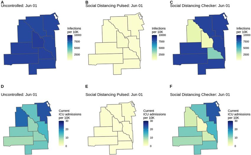
www.nature.com/scientificreports/
Figure 1. Overview of the pipeline. The pipeline has four modules, each with specific inputs that can be
specified by the user. First, we identify when and in which model locations epidemics are seeded using an
air importation model or confirmed case data. Second, the epidemic seeding events are used to initiate the
disease transmission model, which is informed by our epidemiological assumptions and intervention scenarios.
The disease transmission model produces daily incident infection counts and infection prevalence. Next, we
calculate health outcomes like hospitalizations and ICU admissions from these infection counts according to
assumptions about health outcome risks and infection fatality ratios. Finally, these health outcomes may be
summarized using templates and functions from the report generation component of the pipeline.
Methods
Pipeline at a glance. The pipeline consists of multiple modular components designed to run in sequence to
produce results and reports focused on policy relevant outcomes in any set of geographic locations (i.e., multiple
countries, a single country, a set of subnational administrative units, or a single subnational administrative unit)
(Fig. 1). While the pipeline was developed to be extended, the current core components are (1) epidemic seed-
ing, (2) the transmission model, (3) health outcome generation engine, and (4) report generation.
These modular components of the pipeline fit together because each is composed of multiple pieces: an input
format, an output format, one or more code libraries (where applicable), and a runner script. The standardized
input and output formats ensure that components may be switched out according to user preference without
impacting other phases. The “library” generally contains the core functions for a pipeline component. The script
liaises between the user-defined configuration and the library by choosing which library to use and converting
the input format to a format used by the library.
The pipeline runs these components in sequence, according to the specifications outlined in a configuration
file. This makes it easy to add or modify a component. To add a component, we specify its input format, and
incorporate its dependencies. To modify the implementation of a component, we add or modify functions in the
library and function calls in the runner script. When appropriate, entire components may be substituted with data
from outside of the pipeline, provided that the data meet the input formats required by the next pipeline phase.
Module 1: Epidemic seeding and initialization. “Epidemic seeding” refers to how the disease trans-
mission module is initialized with infected individuals. A seeding module must produce one of more seeding
files that specifies an added number of incident cases occurring due to “seeding” at particular dates and locations.
The pipeline currently contains two epidemic seeding options: (1) seeding according to first case appearance
in data, and (2) seeding according to an air travel importation model.
Seeding according to earliest identified cases. This seeding option enables users to seed the model according to
COVID-19 case data. It currently supports user-supplied data and downloads from two commonly used public
sources, the Johns Hopkins University Center for Systems Science and Engineering (JHU-CSSE) COVID-19
Dashboard9 and USAFacts, a database that collates data from US state health departments10. Drawing from the
user-specified data source, this option identifies the first five days that cases were reported in each modeled loca-
tion. We assume that confirmed cases were infected a user-specified number of days prior to when they were
reported, and that there is a user-specified ratio of infections to confirmed cases. Seed infections are, hence,
created in each modeled location on the estimated days of infection for the first 5 days with reported cases; they
are drawn stochastically from a Poisson distribution where the mean is the product of the number of reported
cases and the user-specified ratio.
To facilitate the generation of the seeding file for US settings, we provide the “R/scripts/create_seeding.R”
script in “HopkinsIDD/COVIDScenarioPipeline,” which pulls data directly from USAFacts.
Seeding according to an air importation model. We adapted a previously published model of measles importa-
tion to model the rate of COVID-19 importation to specific locations due to air travel11. This seeding option,
available in the Github repository “HopkinsIDD/covidImportation”12, uses complete itinerary (origin to final
AG13 for all airports in the world, source location populations, and
destination) air travel volume data from O
Scientific Reports | (2021) 11:7534 | https://doi.org/10.1038/s41598-021-86811-0 2
Vol:.(1234567890)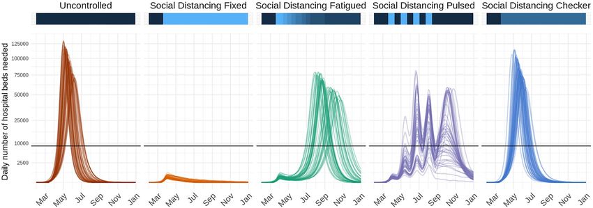
www.nature.com/scientificreports/
source location incidence data, to inform a model with which absolute counts of importation are estimated on
a daily basis into airports12.
Geographic areas surrounding airports are classified spatially into “airport catchment areas” with a Voro-
noi tessellation of space in reference to the latitude and longitude coordinates of the a irport14. When there are
multiple airports within close proximity, the user may specify a threshold distance under which airports may
be grouped into a single cluster that is defined by its centroid. We then assign a probability of importation to
each intersection of a Voronoi tile and an administrative unit boundary. This probability is calculated as the
proportion of the airport catchment area population that lives in that intersection, assuming that population
is distributed evenly by area. All air importations on a given day are then aggregated to the administrative unit
level and seeded into the epidemic model as newly infected individuals.
Module 2: Transmission model and intervention scenarios. The disease transmission module takes
in seeding information and produces an epidemic model output file that contains, at minimum for subsequent
module compatibility, daily counts of incident infections, indexed to their time of symptom onset. The currently
implemented default transmission module comprises a metapopulation model with stochastic Susceptible-
Exposed-Infected-Recovered (SEIR) disease dynamics.
Disease dynamics. The core model is a modified SEIR compartmental model where the time in the “Infected”
compartment follows an Erlang distribution (i.e., the infected compartment is split into k compartments) to
produce more realistic infectious periods where the chance of recovery depends on the time since infection15,
and a coefficient (α) can be set to help the model approximate non-homogeneous mixing between susceptible
and infected individuals and non-exponential growth16. Currently k is fixed at three compartments.
Transition of individuals between disease compartments is simulated stochastically with binomial random
draws:
NS→E (t) = Binom S, 1 − exp (−�t · FOI(t))
NE→I (1) (t) = Binom E, 1 − exp (−�t · σ)
NI(1) →I(2) (t) = Binom I(1) , 1 − exp −�t · γ ′
NI (2) →I (3) (t) = Binom I (2) , 1 − exp −�t · γ ′
NI (3) →R (t) = Binom I (3) , 1 − exp −�t · γ ′
γ′ = γ · k
where S, E, I (1), I (2), I (3), and R represent the number of individuals in those respective compartments, FOI(t) is
the force of infection from the infected population on the susceptible population, σ1 is the latent period, γ1 is the
infectious period, and k is the number of I compartments. The force of infection, which modulates transition of
individuals from the S to E compartments:
k
I (j )
I(t) =
j=1
I(t)α
FOI(t) = β ·
H
k
H = S(t) + E(t) + I (j) (t) + R(t)
j=1
β(t) = R0 · γ
where H is the total population, β is the daily transmission probability as defined by R0 and the infectious period,
and α is the mixing coefficient.
Metapopulation dynamics. The model is capable of simulating disease spread in multiple locations jointly
according to assumptions about population mobility between individual model locations (e.g., administrative
units). The SEIR disease dynamics described above are simulated in each model location with a modification to
the force of infection term that accounts for this impact of mobility on disease spread.
The force of infection in a given location i is calculated from a combination of local infections and infections
in locations that are connected to it according to the mobility matrix, as follows:
Scientific Reports | (2021) 11:7534 | https://doi.org/10.1038/s41598-021-86811-0 3
Vol.:(0123456789)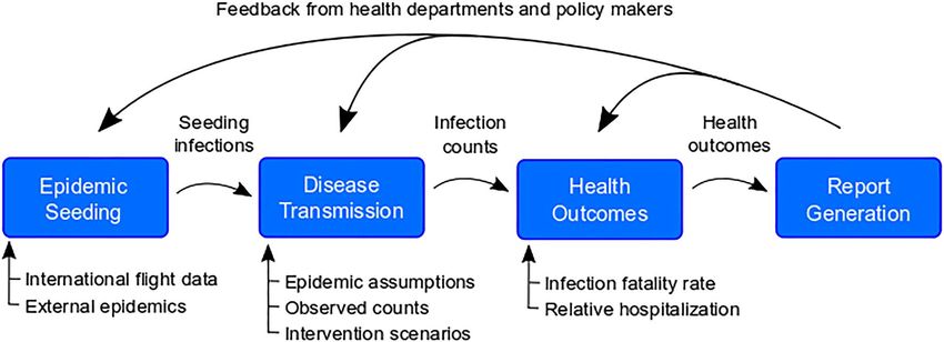
www.nature.com/scientificreports/
Figure 2. Time series of daily number of hospital beds needed across five possible intervention scenarios in a
fictional location with nine counties. Lines represent results from 50 stochastic model simulations. Horizontal
black lines represent the total hospital bed capacity in the fictional location, assumed to be n = 8661 (3 beds
per 1000 population). The colored horizontal bars along the top visualize the effectiveness of interventions at
a given time point along a dark blue to light blue spectrum; dark blue indicates a period with no reductions to
transmission, while light blue indicates a period with more restrictive action (i.e., low transmissibility). In the
fifth scenario, “Social Distancing Checker,” only three of nine counties implement any non-pharmaceutical
interventions, thus differentiating it from “Social Distancing Fixed”.
α � � Mi,j Ij (t)α
�
Mi,j
· βi (t) Ii (t) +
�
FOIi (t) = 1 − pa pa · βj (t)
Hi Hi Hi Hj
j�=i j�=i
where M is a mobility matrix such that Mi,j represents the daily movement of individuals (e.g., commuting)
from origin i to destination j, pa is the proportion of time that moving individuals spend away, and Hi is the
population of node i. The transition of individuals between disease compartments may be modified to index by
location i, for example:
NSi →Ei (t) = Binom Si , 1 − exp (−�t · FOIi (t))
Users may provide a symmetric or asymmetric wide-form mobility matrix for all model locations or a long-
form sparse mobility matrix that indicates only pairs of model locations with connectivity.
Application of transmission modifiers. In the absence of vaccines and other preventive treatments, non-phar-
maceutical interventions, such as school closures, social distancing, stay-at-home directives, and testing and
isolation are critical strategies for reducing disease transmission. Disease transmission may also change across
space or time as the result of exogenous factors like seasonality or spatial heterogeneity in contact patterns. The
model enables users to specify changes to the basic reproductive number ( R0) and the inverse of the infectious
period (γ), for pre-specified periods of time to all or subsets of model locations independently. These interven-
tions or exogenous changes can be implemented with fixed or distributional effectiveness. In addition, users
may specify a rate of fatiguing effectiveness (e.g., declining adherence to a policy) over a certain number of days.
This format enables flexibility in scenario planning; for instance, the model can be used to examine the effects
of chaining multiple interventions together over time (e.g., school closure then stay-at-home), gradual declining
adherence of the population to an intervention, switching interventions on and off over time, spatially heteroge-
neous interventions, or innate spatiotemporal heterogeneities (Fig. 2).
Transmission modifiers like non-pharmaceutical interventions or other exogenous factors modulate the
daily transmission term below:
βi ′ (t) = (1 − ri (t)) · βi (t)
where βi ′ (t) is the daily transmission rate after accounting for transmission modifier ri (t) at the specified location
i at time t. When transmission modifiers are in effect βi′ (t) replaces βi (t) in the force of infection term FOIi (t).
The specification of transmission modifiers is completely user-specified. We include a set of common non-
pharmaceutical intervention scenarios that can be applied for user-specified dates and locations (Table S1), which
have been compiled according to our review of the literature on the potential impact of non-pharmaceutical
interventions on respiratory virus transmission.
Module 3: Calculation of health outcomes. This pipeline module translates outputs from the transmis-
sion model into health outcomes such as hospitalizations and deaths. It takes in counts of daily incident infec-
tions and produces daily counts for specific health outcomes at appropriate time delays.
Scientific Reports | (2021) 11:7534 | https://doi.org/10.1038/s41598-021-86811-0 4
Vol:.(1234567890)www.nature.com/scientificreports/
Column name (notation, as appropriate) Description
p_hosp_inf ( phosp|inf ) Probability of hospitalization among infected individuals
p_icu_hosp (picu|hosp) Probability of ICU admission among hospitalized individuals
p_vent_icu ( pvent|icu) Probability of ventilation among individuals in the ICU
p_death_inf ( pdeath|inf ) Probability of death among infected individuals
rr_hosp_inf Relative risk of hospitalization (given infection) relative to the average across all geoids
rr_death_inf Relative risk of death (given infection) relative to the average across all geoids
Table 1. Health outcome risk parameters.
The current default implementation produces hospital and intensive care unit (ICU) admissions, current
hospital and ICU occupancy, ventilators needs, and number of deaths. Our modeling of health outcomes assumes
that there is some transition probability from infection to death, infection to hospitalization, hospitalization to
ICU admission, and ICU admission to ventilator use. In our modeling of health outcomes, we consider the prob-
ability of its occurrence (e.g., probability that infections are hospitalized), the time delay relative to its disease
course (e.g., time between hospital admission and ICU admission), and where applicable, the duration in a given
state (e.g., how long a patient remains ventilated).
For settings where hospitalization, ICU admission, and ventilator use is infrequent, it may be more appropri-
ate to think of these health outcome projections as different levels of disease severity.
The user may specify health outcome probabilities and delays, conditional on the flows described above.
For use as default values, we provide tables of parameter values which were derived from a literature review of
COVID-19 health outcomes (Table S2).
The pipeline currently contains two versions of this module with different approaches to the specification of
health outcome risks: (1) unadjusted, uniform risk and (2) location-specific risks, adjusted by key demographic
or health factors in each location.
Unadjusted, population‑wide health outcome risks. This option generates health outcome estimates with unad-
justed risk across all locations, assuming fixed values for all health outcome probabilities, delays and durations.
We assumed that the number of infections admitted to the hospital is a draw from the Binomial distribution,
lagged by a fixed time from symptom onset to hospital admission:
hosp
ntinf +tinf→hosp ∼ Binom ninf
tinf , phosp|inf
where nhosp is the number of hospital admissions, ninf is the number of infections, tinf is the time of infection,
tinf→hosp is the mean time delay between infection and hospital admission, and phosp|inf is the probability of
hospitalization given infection (Table 1).
We make similar assumptions for the transitions between other outcomes (hospitalization admission to ICU
admission, ICU admission to ventilator use, infection to death):
hosp
nicu
thosp +thosp→icu ∼ Binom nthosp , picu|hosp
icu
nvent
ticu +ticu→vent ∼ Binom nticu , pvent|icu
inf
ndeath
tinf +tinf→death ∼ Binom ntinf , pdeath|inf
The number of patients currently hospitalized, admitted to ICU, and ventilated are generated from the inci-
dent number of events and fixed (non-distributional) user-defined durations for each event.
As information about the death and hospitalization rates were scarce early on in the pandemic, decision
makers wanted to consider how things would unfold over different scenarios of health burden. To facilitate
these needs, our pipeline separates hospitalization and death rates from the other outcomes, and allows users to
consider multiple scenarios for different rates.
Location‑specific health outcome risks. The severity of disease from SARS-CoV-2 infection can vary greatly
between locations due to difference between populations; individuals that are older, with limited access to health
care, or with certain pre-existing health conditions are at greater risk for severe disease and death. For this
reason, the hospitalization module also supports the specification of location-specific relative risks, which can
be used, for example, to standardize hospitalization and mortality rates according to the age distribution of the
population. Users may provide a wide format data file with standardized variable names for the transition prob-
abilities and relative risks (columns) by geoid (rows). These transition probabilities are conditional on previous
states (e.g., probability of hospitalization given infection is named p_hosp_inf). The probability of hospitaliza-
tion and death given infection are specified as relative values compared to population-wide averages specified
Scientific Reports | (2021) 11:7534 | https://doi.org/10.1038/s41598-021-86811-0 5
Vol.:(0123456789)www.nature.com/scientificreports/
in the configuration file. We note that the location-specific standardizations apply only to the health outcomes,
making a critical assumption that all individuals are at equal risk of infection.
While location-specific data is not required to differ for all health outcome transition probabilities (i.e., some
probabilities can be constant across all locations), the location-specific file should include the variables described
in Table 1 and population-wide average values for the probability of hospitalization (p_hosp_inf) and death
(p_death_inf) given infection.
To facilitate construction of such files, we have created a companion package covidSeverity that
produces location-specific relative death and hospitalization rates based on the age distribution of the local
population17. The package generates these outputs for US counties based on data from the US Census Bureau, and
we provide this as a model input file as part of the main pipeline implementation (see COVIDScenarioPipeline/
sample_data/geoid-params.csv). The package also includes built-in functionality to pull data from W orldPop18
and generate adjustments for any location of interest17.
The covidSeverity package applies a logistic generalized additive model (GAM) with a penalized cubic
spline for age and random effect for age-specific estimates of risk of each health outcome from the literature, thus
producing estimates of risk for 10-year, aggregated age categories. These age-specific estimates are then applied
to the population age distribution in a given location.
Module 4: Summarization of model outputs. This component of the pipeline provides wrapper func-
tions for the lightweight summarization of model outputs into quantiles, plotting functions for common figures,
and R Markdown templates to facilitate the rapid generation of technical reports. This module is available in the
R package report.generation in the Github repository “HopkinsIDD/COVIDScenarioPipeline.”
We provide two key functions that read and process individual transmission (load_scenario_sims_
filtered) and health outcome (load_hosp_sims_filtered) model output files. In managing individual
files with these functions, we reduce the processing time and memory load. Both of these functions take pro-
cessing functions as arguments, thus enabling aggregation and filtering to occur at the level of individual files.
The package contains technical report R Markdown templates for US states, US counties, and individual
countries, a diagnostic report template called “sanity_check_report,” and a template that is maintained solely
for integration testing. When report.generation is installed and loaded, the templates become available
to the user. Many parameters are drawn from the configuration file automatically and pre-written R Markdown
chunks about the module options and methods can be referenced within the package.
Common figures include summary tables and time courses for estimated health outcomes under different
interventions, maps that portray cumulative cases at the county level, comparisons between model estimates and
observed cases and deaths, and visualizations for when ICU and ventilator capacity for each county is exceeded.
The vignette below walks through example report outputs in more detail and we provide a template-generated
report example in the “Supplementary Material” (Example Report).
Model specification. All components and settings for simulations from the COVID Scenario Pipeline
model are specified in an easily-modifiable YAML configuration file. We describe different options in detail in the
Results and an example of the complete set of configuration options is provided in the “Supplementary Material”.
Model access and use. The project is open-source under the GNU General Public License v3.0 license,
and code is available at https://github.com/HopkinsIDD/COVIDScenarioPipeline. The master branch of this
repository consists of a Python package “SEIR” and two R packages “hospitalization” and “report.generation,”
which correspond to the second, third, and fourth modules of the model pipeline (https://zenodo.org/badge/
latestdoi/245866576). Air importation-based seeding is implemented in the covidImportation package
(https://github.com/HopkinsIDD/covidImportation), while seeding according to the earliest identified cases is
performed in scripts within the “HopkinsIDD/COVIDScenarioPipeline” repository.
Results: scenario modeling vignette
Here, we present a vignette with 50 model simulations in a fictional setting (Location X) with nine counties
(named A through I) in demonstrative intervention scenarios from January 31 to December 31, 2020. In this
vignette, we walk through how to set up and run the pipeline, demonstrate some of the spatial and temporal
features for modeling non-pharmaceutical interventions, and display some of the plotting functions useful for
summarizing the model output.
To run the model, users will require the functionality of the “HopkinsIDD/COVIDScenarioPipeline” reposi-
tory and a second GitHub repository specific to their model location. A template for such a spatial repository
may be found at “HopkinsIDD/COVID19_Minimal” (https://github.com/HopkinsIDD/COVID19_Minimal),
and complete details on downloading and running the model are available in the template’s wiki at https://g ithub.
com/HopkinsIDD/COVID19_Minimal/wiki.
Once we have a working environment, the next step is to create a configuration file to describe the model
specifications. A skeleton configuration file is included in the COVID19_Minimal template, and the full con-
figuration file accompanying the results of this vignette is in the “Supplementary Material”.
First, we specify the broad parameters of the run, such as the date range covered and the number of simula-
tions to run (see first section in “Supplementary Material”, Example YAML Configuration File).
Next we provide spatial setup information identifying the location of files containing geographic data and
the geographic targets for modeling. The spatial_setup section of the configuration file identifies a geo-
graphical data (geodata) file that contains the population data for each county or administrative subunit in the
location(s) of interest and a mobility matrix file that contains the daily trip counts for each pair of counties. Users
Scientific Reports | (2021) 11:7534 | https://doi.org/10.1038/s41598-021-86811-0 6
Vol:.(1234567890)www.nature.com/scientificreports/
may employ the R scripts “build_US_setup.R” or “build_nonUS_setup.R,” which are provided with the reposi-
tory, to generate compatible geodata and mobility matrix files. For users modeling non-US settings, the Github
repository “COVID-19-Mobility-Data-Network/mobility” can be used to fit real-time or sparse travel data with
mobility models in order to generate similarly compatible mobility m atrixes19,20.
We note that in situations with high cross-border mobility, it may be important to model a region larger than
the location of interest in order to appropriately capture disease transmission risk in a given location. Here, we
model Locations X, Y, and Z even though Location X is the sole location of interest:
spatial_setup:
base_path: data/location-x ## base path to spatial files
setup_name: location-x ## spatial folder name
geodata: geodata.csv ## path to geodata file with modeled geoids
mobility: mobility.csv ## path to mobility matrix
popnodes: pop ## column name of population in geodata
nodenames: geoid ## column name of unique location identifiers in geodata
modeled_states:
-X
-Y
-Z
We then specify the locations of the seeding files (see seeding section in “Supplementary Material”, Example
YAML Configuration File), with a separate section to describe the air importation model parameters as appropri-
ate (see importation in “Supplementary Material”, Example YAML Configuration File).
Next, we specify the parameters that determine the course of the disease. The seir section of the configura-
tion file defines parameters used in the SEIR disease transmission model, including the level of population mixing
(where 1 is homogeneous mixing, and < 1 is heterogeneous), the incubation period of the virus, the infectious
period, and the baseline basic reproductive number R0. These values may be fixed or drawn randomly from a
distribution, according to the configuration file:
seir:
parameters:
alpha: 1 ## mixing coefficient
sigma: 1 / 5.2 ## inverse of the incubation period in days
gamma: ## inverse of the infectious period in days
distribution: uniform
low: 1 / 6
high: 1 / 2.6
R0s: ## baseline basic reproductive number
distribution: uniform
low: 2
high: 3
We typically parameterize sigma and gamma in our model with estimates of the range of the serial interval
(SI) or generation time, such that
1 1 1
SI = + ,
2 γ σ
which assumes that the average infection occurs halfway through an index case’s infectious period.
The next step is defining the modeled intervention scenarios. Here, we considered five scenarios in our
vignette example: (1) a no intervention scenario (named Uncontrolled), in which R0 remains unchanged
over the course of the outbreak; (2) social distancing measures with fixed effectiveness in place from March 19
to December 31 (SocialDistancing_fixed); (3) social distancing measures with declining compliance,
which were modeled as 10% reductions in effectiveness every 2 weeks beginning March 19 (SocialDistanc-
ing_fatigued); (4) social distancing measures following a 3-week on–off “pulsing” cycle from March 19 to
August 12 (SocialDistancing_pulsed); and (5) social distancing measures with spatial heterogeneity
(SocialDistancing_checker), where three of nine counties implement social distancing measures with
fixed effectiveness from March 19 to December 31.
An intervention may be specified in a single block for all model locations, as in the case of the Social-
Distancing_fixed scenario, or for unique location identifiers (“geoids”) as in the SocialDistanc-
ing_checker scenario:
Scientific Reports | (2021) 11:7534 | https://doi.org/10.1038/s41598-021-86811-0 7
Vol.:(0123456789)www.nature.com/scientificreports/
SocialDistancing_fixed: ## scenario name
template: ReduceR0
period_start_date: 2020-03-19 ## intervention start date
period_end_date: 2020-12-31 ## intervention end date
value: ## randomly draw an intervention effectiveness value from a uniform distribution
between .71 and .83
distribution: uniform
low: .71
high: .83
SocialDistancing_checker:
template: ReduceR0
affected_geoids: ["County B", "County E", "County F"] ## matches location IDs in geodata
file
period_start_date: 2020-03-19
period_end_date: 2020-12-31
value:
distribution: uniform
low: .71
high: .83
Other intervention scenarios require multiple blocks to be stacked together, as in the case of the Social-
Distancing_pulsed scenario, shown in truncated form below:
SD_Pulse1:
template: ReduceR0
period_start_date: 2020-03-19
period_end_date: 2020-04-08
value:
distribution: uniform
low: .71
high: .83
SD_Pulse2:
template: ReduceR0
period_start_date: 2020-04-30
period_end_date: 2020-05-20
value:
distribution: uniform
low: .71
high: .83
... ...
SocialDistancing_pulsed:
template: Stacked
scenarios:
- SD_Pulse1
- SD_Pulse2
- SD_Pulse3
- SD_Pulse4
Then, we set up the health outcome risk specifications. In the hospitalization section of the con-
figuration file, we specify whether the model calculates health outcome risks with age-adjusted estimates, the
average infection fatality ratios (IFR), and the time delays between different health outcomes. The time delays
are modeled with lognormal distributions and parameterized with the log median and log standard deviation.
For ease of use, we provide a table of estimates found in the literature in Table S2.
After the simulation runs complete, we can produce rapid summaries of the results using R Markdown tem-
plates provided by the report.generation package. The report section of the configuration file specifies
scenario labels and colors, IFR scenario labels, and table display dates. These settings, along with other model
parameters, can be loaded into a technical report template.
Here we describe how the state_report template in the report.generation package can be used
to display our model results as an example. The full template-generated report linked to this vignette is provided
in the “Supplementary Material” (Example Report). First, the configuration file is loaded to pull in the model
settings and file paths. Then, we use a number of predefined functions to load and plot the data.
For example, one standard report figure compares time series of the daily number of hospital beds needed
across intervention scenarios (Fig. 2) using the load_hosp_geocombined_totals and plot_ts_
hosp_state_sample functions from the report.generation package in order to load and plot the
Scientific Reports | (2021) 11:7534 | https://doi.org/10.1038/s41598-021-86811-0 8
Vol:.(1234567890)www.nature.com/scientificreports/
data. To plot variations of these figures, we only need to change which health outcome variable is specified in
plot_ts_hosp_state_sample.
While Fig. 2 displays aggregate results, our reports also provide location-specific risk and logistical outputs
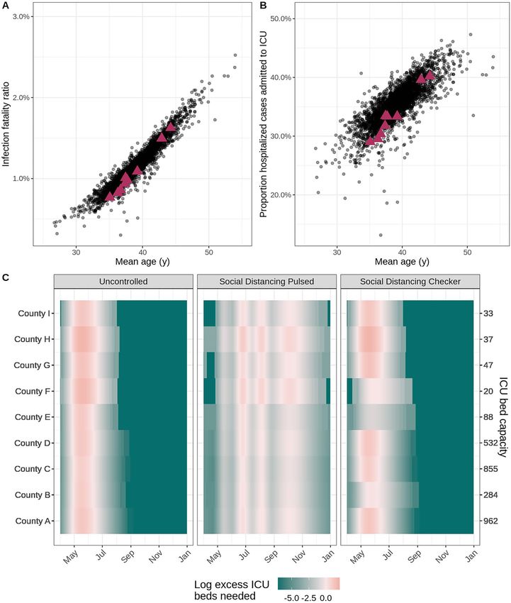
at the county- or administrative subunit-level. For example, we present the age-adjusted infection fatality ratios
and risk of ICU admission among hospitalized infections for the modeled counties within the distribution of all
counties in the United States in Fig. 3A,B. Using the load_hosp_geounit_relative_to_threshold
and plot_needs_relative_to_threshold_heatmap functions from report.generation, we
display the potential need for beds in excess of health system capacity by model location in our reports (Fig. 3C).
Values of the location-specific healthcare capacity, represented by the number of staffed hospital, acute care, or
intensive care beds available and/or number of ventilators available, are user-defined; these can be based on
assumptions of the average availability per person or input from data where available.
A map of model outputs makes it easier to visualize spatial and temporal heterogeneity in different inter-
vention scenarios (Fig. 4). We provide this functionality in the load_cum_inf_geounit_dates and
plot_geounit_map functions in the report.generation package.
Each report template is equipped to load static R Markdown reference chunks, which we have pre-written
and provided with the package. These chunks provide details on our methods, limitations, and key references,
pulling in parameters from the configuration file as needed.
Discussion
We present our scenario pipeline as an open-source modeling framework that aims to balance epidemiological
rigor with the flexibility and urgency required by public health policymaking. The modularity of our framework
has enabled us to adapt our assumptions about COVID-19 epidemiology, transmission, and health outcome risks
in response to emerging information and to different settings. The pipeline implementation of non-pharmaceu-
tical interventions is highly adaptable for policymakers desiring to compare the impact of different potential
scenarios.
Throughout the course of the pandemic, we have adapted the default settings of our pipeline in response to
the changing needs and questions of our collaborators. At the beginning of the pandemic, air importation seed-
ing was a critical determinant of epidemic onset in specific locations. Now that cases of COVID-19 are present
worldwide, we have shifted towards developing more empirical methods of epidemic seeding that better match
trajectories of confirmed cases in specific locations as policy questions have shifted to more operational needs.
As new data emerged, we moved from calculating unadjusted health outcomes to health outcomes based on
age-standardized risk of hospitalization, ICU admission, and death according to emerging case-study data.
As the COVID-19 pandemic continues, we plan to continue expanding the scope of the COVID Scenario
Pipeline to changing needs and questions. Future model releases will include a health outcomes model expan-
sion that will enable a multiplicity of pathways to ICU occupancy, ventilator usage, and death. As questions
have shifted to near-term operational needs, we have also begun to incorporate inference into our models, thus
enabling the calibration of model trajectories to deaths and confirmed case counts, short-term forecast of health
outcomes, and estimation of location-specific transmission parameters and NPI effectiveness.
While the pipeline’s generic structure means that different modules may be readily replaced, the current
implementation of our model has several limitations with regard to the epidemiology of COVID-19. The disease
transmission model does not explicitly incorporate age-specific contact or transmission rates or asymptomatic
transmission, nor does it consider how factors like testing rates may lead to time-varying biases in reporting.
Data to inform these factors was scarce when this model was initially developed, but these processes can change
the dynamics displayed by scenario projections. Moreover, this model structure means that we cannot model
age-targeted interventions (e.g., cocooning of high-risk age groups) or interventions targeting asymptomatic
individuals (e.g., systematic age-specific testing) in a mechanistic manner. However, we can and do adjust for
these types of interventions through overall population-level reductions in disease transmission. Additionally,
the current model cannot tune changes in population mobility or connectivity over time, although we know that
travel and movement restrictions played a role in changing the spread of COVID-19.
The health outcomes module also has several structural limitations; we assume that only one progression
in health outcome severity exists (infection to hospitalization to ICU to ventilator use), although we know that
many disease course progressions are possible. In addition, the delays and durations involved in our health
outcomes progression are fixed in time for a given location, although stochastic variation may be incorporated
across simulations..
Nevertheless, the modular approach taken is meant to allow for easy substitution of models with improve-
ment in any of these areas while still taking advantage of other pipeline components. We have leveraged this
feature throughout the course of the COVID-19 pandemic, and individual modules continue to develop. This
flexibility does come at a cost, as the modular pipeline approach requires us to write and read files at the end and
beginning of each phase, respectively. This procedure requires more disk space and input/output steps than other
modeling approaches that can hold all of the necessary data in memory until a single output is produced at the
end. Still, these slowdowns are not critically limiting; we have been able to run 1000 county-level simulations of
the United States in less than 10 min on a 96 core server.
These limitations point to a broader need to consider the totality of evidence generated by epidemiologic
models. While our approach is well-suited to answering policy questions about interventions, it is critical for
policymakers to explore projections from multiple models in order to understand the range of possible trajec-
tories and the sensitivity of results to different assumptions. Models that incorporate individual-level behaviors
may be better for considering the impact of specific contact tracing strategies or location-specific measures like
workplace occupancy or symptom screening policies that are not well captured in compartmental models such
Scientific Reports | (2021) 11:7534 | https://doi.org/10.1038/s41598-021-86811-0 9
Vol.:(0123456789)www.nature.com/scientificreports/
Figure 3. Health outcome risks and logistical needs for fictional counties. In the scatterplots, each point
indicates (A) the age-adjusted infection fatality ratio and (B) risk of ICU admission given hospitalization by
mean age for a county within the United States. Data for the nine fictional counties in our vignette is marked
by magenta triangles. (C) The heat maps display county-level ICU bed needs, shaded according to the log ratio
above or below the assumed ICU bed capacity (secondary y-axis) in each county (primary y-axis) for three
example intervention scenarios (panels). The salmon pink shading indicates periods of time where ICU bed
needs exceed capacity in the fictional counties.
as ours21–23. Other individual-based models are better suited for addressing heterogeneities due to differences
in household or social structures24,25. Models incorporating real-time mobility data can best characterize the
impact of movement-related restrictions26 models with age-specific transmission may provide more detail on
the impact of age-specific interventions like “cocooning”27 or closing and opening s chools4. Still other models
are particularly suited to address questions about health systems burden and forecast operational n eeds5,28,29 and
to consider the economic impacts of transmission and i nterventions30,31. Integrating knowledge from multiple
models, where appropriate, with careful consideration of the assumptions and appropriate applications of each
model, will strengthen response and p reparedness32.
Scientific Reports | (2021) 11:7534 | https://doi.org/10.1038/s41598-021-86811-0 10
Vol:.(1234567890)www.nature.com/scientificreports/
Figure 4. County-level COVID-19 risk for three scenarios (Uncontrolled, Pulsed, Checker) in the fictional
Location X. Choropleths for model outcomes on June 1, 2020 of the (A–C) cumulative infection rate per
10,000 population and (D–F) number of patients currently admitted to the ICU per 10,000 population for
the Uncontrolled, Social Distancing Pulsed, and Social Distancing Checker intervention scenarios. County-
level variation in attack rates can arise from differences in risk of importation, mobility patterns connecting
subdivisions, and differences in non-pharmaceutical interventions applied in each location. If location-specific
health outcome risks are specified (as are age-standardized health outcome risks in this example), this may serve
as another source of county-level variation.
Our flexible modeling pipeline brings an important voice to this “conversation” of models, by allowing rapid
and flexible specification and simulation of even very complex intervention scenarios, and providing flexibility
to rapidly update models as our understanding of a disease changes. This approach only reaches its full potential
when parameters are based on careful and ongoing consideration of the literature and available data. But, when
appropriately used as part of an iterative approach to decision making, this pipeline can be a valuable tool for
public health decision making.
Received: 9 September 2020; Accepted: 18 March 2021
References
1. Zhu, N. et al. A novel coronavirus from patients with pneumonia in China, 2019. N. Engl. J. Med. 382, 727–733 (2020).
2. WHO Director-General’s opening remarks at the media briefing on COVID-19—11 March 2020. in World Health Organization
[Internet]. Accessed 11 Mar 2020 [cited 22 May 2020]. https://www.who.int/dg/speeches/detail/who-director-general-s-openi
ng-remarks-at-the-media-briefi ng-on-covid-19---11-march-2020.
3. Huang, C. et al. Clinical features of patients infected with 2019 novel coronavirus in Wuhan, China. Lancet 395, 497–506 (2020).
4. Ferguson, N., Laydon, D., Gilani, G.N., Imai, N., Ainslie, K., Baguelin, M., et al. Report 9: Impact of non-pharmaceutical interven-
tions (NPIs) to reduce COVID19 mortality and healthcare demand. 2020 [cited 22 May 2020]. https://doi.org/10.25561/77482.
5. Branas, C.C., Rundle, A., Pei, S., Yang, W., Carr, B.G., Sims, S., et al. Flattening the curve before it flattens us: Hospital critical care
capacity limits and mortality from novel coronavirus (SARS-CoV2) cases in US counties. medRxiv (2020) https://d oi.o
rg/1 0.1 101/
2020.04.01.20049759.
6. Moghadas, S. M. et al. Projecting hospital utilization during the COVID-19 outbreaks in the United States. Proc. Natl. Acad. Sci.
USA 117, 9122–9126 (2020).
7. Davies, N.G., Klepac, P., Liu, Y., Prem, K., Jit, M., CMMID COVID-19 Working Group, et al. Age-dependent effects in the trans-
mission and control of COVID-19 epidemics. Nat Med 26, 1205–1211 (2020). https://doi.org/10.1038/s41591-020-0962-9.
8. IHME COVID-19 Health Service Utilization Forecasting Team, Murray, C.J.L. Forecasting the impact of the first wave of the
COVID-19 pandemic on hospital demand and deaths for the USA and European Economic Area countries. medRxiv (2020) https://
doi.org/10.1101/2020.04.21.20074732.
Scientific Reports | (2021) 11:7534 | https://doi.org/10.1038/s41598-021-86811-0 11
Vol.:(0123456789)www.nature.com/scientificreports/
9. Dong, E., Du, H. & Gardner, L. An interactive web-based dashboard to track COVID-19 in real time. Lancet Infect Dis. 20, 533–534
(2020).
10. "US COVID-19 cases and deaths by state" in USA Facts [Internet]. [cited 23 May 2020]. usafacts.org.
11. Truelove, S.A., Mier-y-Teran-Romero, L., Gastanaduy, P., Taylor Walker, A., Berro, A., Lessler, J., et al. Epidemics, air travel, and
elimination in a globalized world: The case of measles. medRxiv (2020) https://doi.org/10.1101/2020.05.08.20095414.
12. Truelove, S., Lauer, S.A., Lemaitre, J., Kaminsky, K., Kaminsky, J. HopkinsIDD/covidImportation: Initial release of covidImporta-
tion R package. (2020). [cited 23 May 2020]. https://doi.org/10.5281/zenodo.3840560.
13. Flight data in OAG [Internet]. [cited 23 May 2020]. oag.com.
14. Balcan, D. et al. Modeling the spatial spread of infectious diseases: The GLobal Epidemic and Mobility computational model. J.
Comput. Sci. 1, 132–145 (2010).
15. Yan, P. & Chowell, G. Quantitative methods for investigating infectious disease outbreaks. Texts Appl. Math. https://doi.org/10.
1007/978-3-030-21923-9 (2019).
16. Finkenstädt, B. F., Bjørnstad, O. N. & Grenfell, B. T. A stochastic model for extinction and recurrence of epidemics: Estimation
and inference for measles outbreaks. Biostatistics 3, 493–510 (2002).
17. Lauer, S.A., Truelove, S.A., Grantz, K. HopkinsIDD/covidSeverity: Initial release of covidSeverity R package. (2020) [cited 23 May
2020]. https://doi.org/10.5281/zenodo.3840716.
18. "Population counts" in WorldPop [Internet]. [cited 24 May 2020]. https://www.worldpop.org/.
19. Giles, J. COVID-19-Mobility-Data-Network/mobility: v0.1.1 alpha release of mobility R package. (2020) [cited 23 May 2020].
https://doi.org/10.5281/zenodo.3838719.
20. Giles, J. and Wesolowski, A. mobility: an R package for modeling human mobility patterns. [cited 23 May 2020]. https://covid-19-
mobility-data-network.github.io/mobility/index.html.
21. Kucharski, A. J. et al. Effectiveness of isolation, testing, contact tracing, and physical distancing on reducing transmission of SARS-
CoV-2 in different settings: A mathematical modelling study. Lancet Infect. Dis. 20, 1151–1160 (2020).
22. Firth, J. A. et al. Using a real-world network to model localized COVID-19 control strategies. Nat. Med. 26, 1616–1622 (2020).
23. Hinch, R., Probert, W.J.M., Nurtay, A., Kendall, M., Wymatt, C., Hall, M., et al. OpenABM-Covid19—An agent-based model for
non-pharmaceutical interventions against COVID-19 including contact tracing. medRxiv (2020) https://doi.org/10.1101/2020.
09.16.20195925.
24. Wilder, B. et al. Modeling between-population variation in COVID-19 dynamics in Hubei, Lombardy, and New York City. Proc.
Natl. Acad. Sci. USA 117, 25904–25910 (2020).
25. Kerr, C. C. et al. Covasim: An agent-based model of COVID-19 dynamics and interventions. medRxiv (2020) https://doi.org/10.
1101/2020.05.10.20097469.
26. Lai, S., Ruktanonchai, N.W., Zhou, L., Prosper, O., Luo, W., Floyd, J.R., et al. Effect of non-pharmaceutical interventions to contain
COVID-19 in China. Nature 585, 410–413 (2020).
27. Duque, D., Morton, D.P., Singh, B., Du, Z., Pasco, R., Meyers, L.A. COVID-19: How to relax social distancing if you
must. medRxiv (2020) https://doi.org/10.1101/2020.04.29.20085134.
28. Los Alamos National Laboratory. COVID-19 Cases and Deaths Forecasts. [cited 24 May 2020]. https://covid-19.bsvgateway.org/.
29. Weissman, G. E. et al. Locally hospital informed simulation to predict capacity needs during the COVID-19 pandemic. Ann. Intern.
Med. 173, 21–28 (2020).
30. Acemoglu, D., Chernozhukov, V., Werning, I., Whinston, M. D. Optimal targeted lockdowns in a multi-group SIR model. National
Bureau of Economic Research, Working Paper 27102 (2020). http://www.nber.org/papers/w27102.
31. Silva, P. C. L. et al. COVID-ABS: An agent-based model of COVID-19 epidemic to simulate health and economic effects of social
distancing interventions. Chaos Solitons Fractals. 139, 110088 (2020).
32. Shea, K. et al. Harnessing multiple models for outbreak management. Science 368, 577–579 (2020).
Acknowledgements
We acknowledge technical support from Amazon Web Services, with particular thanks to Pierre-Yves Aquilanti,
Karthik Raman, Arun Subramaniyan, Greg Thursam, and Anh Tran for their time and expertise.
Author contributions
K.H.G., J.K., H.R.M., S.A.T., L.T.K., J.L., and E.C.L. wrote the first draft of the manuscript. J.C.L., J.K., K.H.G.,
and S.A.T. wrote the core model code. K.H.G. and H.R.M. prepared the manuscript figures. H.R.M. prepared
the supplementary material. S.S., J.W., K.K., and J.P.S. contributed to model and code optimization and docu-
mentation. J.L. and E.C.L. guided the design, analysis, and execution of the project. J.C.L., K.H.G., J.K., H.R.M.,
S.A.T., S.A.L., L.T.K., J.P.-S., J.L., and E.C.L. contributed to study design and analysis. All authors contributed
model code and reviewed the manuscript.
Funding
JCL, KHG, JK, HRM, SAT, SAL, LTK, JPS, JL, and ECL were supported by the State of California. JCL, JK, SAT,
SAL, LTK, JPS, JL, and ECL were supported by the US Department of Health and Human Services and the US
Department of Homeland Security. JCL acknowledges funds provided by the Swiss National Science Foundation
(200021-172578) and the attached mobility Grant. SAT acknowledges funds provided by the US Office of Foreign
Disaster Assistance (130492) and the Centers for Disease Control and Prevention (126280). LTK acknowledges
funds provided by the Centers for Disease Control and Prevention (5U01CK000538-03) and the University of
Utah Immunology, Inflammation, & Infectious Disease Initiative (26798 Seed Grant). This work was also sup-
ported with computing service credits from Amazon Web Services and more generally by the Johns Hopkins
Health System and the Office of the Dean at the Johns Hopkins Bloomberg School of Public Health.
Competing interests
The authors declare no competing interests.
Additional information
Supplementary Information The online version contains supplementary material available at https://doi.org/
10.1038/s41598-021-86811-0.
Correspondence and requests for materials should be addressed to E.C.L.
Scientific Reports | (2021) 11:7534 | https://doi.org/10.1038/s41598-021-86811-0 12
Vol:.(1234567890)www.nature.com/scientificreports/
Reprints and permissions information is available at www.nature.com/reprints.
Publisher’s note Springer Nature remains neutral with regard to jurisdictional claims in published maps and
institutional affiliations.
Open Access This article is licensed under a Creative Commons Attribution 4.0 International
License, which permits use, sharing, adaptation, distribution and reproduction in any medium or
format, as long as you give appropriate credit to the original author(s) and the source, provide a link to the
Creative Commons licence, and indicate if changes were made. The images or other third party material in this
article are included in the article’s Creative Commons licence, unless indicated otherwise in a credit line to the
material. If material is not included in the article’s Creative Commons licence and your intended use is not
permitted by statutory regulation or exceeds the permitted use, you will need to obtain permission directly from
the copyright holder. To view a copy of this licence, visit http://creativecommons.org/licenses/by/4.0/.
© The Author(s) 2021
Scientific Reports | (2021) 11:7534 | https://doi.org/10.1038/s41598-021-86811-0 13
Vol.:(0123456789)You can also read