Multi-model ensemble of statistically downscaled GCMs over southeastern South America: historical evaluation and future projections of daily ...
←
→
Page content transcription
If your browser does not render page correctly, please read the page content below

Multi-model ensemble of statistically downscaled
GCMs over southeastern South America: historical
evaluation and future projections of daily
precipitation with focus on extremes
Matias Ezequiel Olmo ( molmo@at.fcen.uba.ar )
Universidad de Buenos Aires Facultad de Ciencias Exactas y Naturales https://orcid.org/0000-0003-
3324-9040
Rocio Balmaceda-Huarte
University of Buenos Aires: Universidad de Buenos Aires
Maria Laura Bettolli
University of Buenos Aires: Universidad de Buenos Aires
Research Article
Keywords: statistical downscaling, extreme rainfall, southeastern South America, CMIP5, CMIP6, climate
change
Posted Date: October 1st, 2021
DOI: https://doi.org/10.21203/rs.3.rs-942877/v1
License: This work is licensed under a Creative Commons Attribution 4.0 International License.
Read Full License
Page 1/30
Abstract
High-resolution climate information is required over southeastern South America (SESA) for a better
understanding of the observed and projected climate changes due to their strong socio-economic and
hydrological impacts. Thereby, this work focuses on the construction of an unprecedented multi-model
ensemble of statistically downscaled global climate models (GCMs) for daily precipitation, considering
different statistical techniques - including analogs, generalized linear models and neural networks - and a
variety of CMIP5 and CMIP6 models. The skills and shortcomings of the different downscaled models
were identified. Most of the methods added value in the representation of the main features of daily
precipitation, especially in the spatial and intra-annual variability of extremes. The statistical methods
showed to be sensitive to the driver GCMs, although the ESD family choice also introduced differences in
the simulations. The statistically downscaled projections depicted increases in mean precipitation
associated with a rising frequency of extreme events - mostly during the warm season - following the
registered trends over SESA. Change rates were consistent among downscaled models up to the middle
21st century when model spread started to emerge. Furthermore, these projections were compared to the
available CORDEX-CORE RCM simulations, evidencing a consistent agreement between statistical and
dynamical downscaling procedures in terms of the sign of the changes, presenting some differences in
their intensity. Overall, this study evidences the potential of statistical downscaling in a changing climate
and contributes to its undergoing development over SESA.

1. Introduction
Emerging recognition has lately been seen on precipitation extremes that occur over southeastern South
America (SESA, roughly between 50–65 °W and 20–40 °S), since SESA stands out as one of the regions
where extreme events are becoming more frequent and intense (IPCC, 2021). By being immersed over La
Plata basin, the main socio-economic activities in SESA rely on the exploitation of water resources such
as rainfed agriculture, hydro-power generation and river transportation. In addition, extreme precipitation
events are one of the main contributors to the SESA precipitation annual cycle, triggering the overflow of
the main rivers and largely extended floods (Vörösmarty et al. 2013). According to the literature, the
positive trends on precipitation and the extremes registered in the recent period are expected to intensify
during the late 21st century as global warming conditions enhance the water vapor availability necessary
for the development of precipitation systems (Blázquez and Solman, 2020; Li et al. 2020; Díaz et al. 2020;
Olmo et al. 2020; Torres et al. 2021; Almazroui et al. 2021).

In a climate change scenario, local adaptation and mitigation policies require the availability of possible
evolutions of meteorological variables linked to different climate hazards, such as extreme precipitation.
In spite of the significant advances in simulating the Earth’s climate by global climate models (GCMs) -
from paleoclimatic scenarios, recent and future changes - the uncertainties in future climate projections
are still large. This is due to different puzzling aspects of climate modelling such as the variety of climate
models and parametrizations, emission scenarios and natural variability (Lehner et al. 2020). The climate
scientific community is devoted to the development and evaluation of different modelling procedures to
                                                  Page 2/30
obtain an optimal representation of the physical mechanisms that control the climatic system. In this
context, the Coupled Model Intercomparison Projects (CMIPs) provide essential tools for a better
understanding of the climate changes that arise from natural variability or in response to changes in
radiative forcing. These intercomparison efforts provide long-term historical runs covering much of the
industrial period, from 1850 to 2005 in the CMIP version 5 (CMIP5) and to 2014 in CMIP6 (Taylor et al.,
2012; Eyring et al. 2016). The historical simulations allow us to evaluate model performance during the
present climate, which results useful to quantify the possible causes of the spread in the GCMs future
simulations.

GCMs precipitation outputs typically depict difficulties in reproducing the extreme values - mainly due to
not enough spatial resolution and limited representation of sub-grid scale phenomena - pointing out the
need for generating regional climate information for mitigation and adaptation strategies. In this context,
dynamical and statistical downscaling approaches arise as key procedures required to improve the
representation of regional and local scale features such as extreme rainfall. Particularly, the Coordinated
Regional Climate Downscaling Experiment (CORDEX) initiative is dedicated to the generation of
coordinated and consistent downscaling models over different regions of the world (Gutowski et al.
2016). Dynamical downscaling relies on regional climate models (RCMs), that provide high-resolution
information by numerically simulating the physical processes of the climatic system (Rummukainen,
2010). However, their high demand of computation resources limits the number of RCM outputs available
particularly in domains like South America, where only few modelling institutes can afford to perform
these simulations. In this sense, empirical statistical downscaling (ESD) appears as a powerful tool with
significantly lower computational cost than other downscaling procedures. On this approach, high-
resolution information is obtained by identifying relationships between large-scale predictors and the
predictand surface variable during the observed climate, which are then applied to GCMs simulations
(Maraun et al. 2015). Many studies around the globe have assessed the capability of a variety of ESD
techniques in simulating regional and local climate features (ie, Gutiérrez et al. 2019; Araya-Osses et al.
2020; Sulca et al. 2021; Wang et al. 2021) and in generating future climate projections (ie, Haylock et al.
2006; Vu et al. 2015; Asong et al. 2016; Baño-Medina et al. 2021). Thus, the design of statistical
downscaling strategies becomes of great scientific interest in areas like SESA, where all described above
motivates the study of extreme precipitation events, their impact through hydrological modelling and the
future changes of heavy rainfall. However, the application of ESD methods in studies of spatio-temporal
climate variability and extremes over this region is still emerging. Only few studies have evaluated the
ESD potential for obtaining regional climate information over SESA (D’onofrio et al. 2010, Menéndez et al.
2010; Bettolli and Penalba, 2018; Bettolli et al. 2021; Solman et al. 2021). Nevertheless, the study of
future projections by means of ESD strategies as well as the inspection of the added value of these
downscaled simulations are still open lines of research in the region.

In this way, the present study is based on a recent statistical downscaling experiment of daily
precipitation over SESA (Olmo and Bettolli, 2021b), in which an evaluation of multiple ESD methods -
including novel methodologies for the region like artificial neural networks and circulation-conditioned
generalized linear models - was performed. The authors exhaustively validated the ESD models
                                                  Page 3/30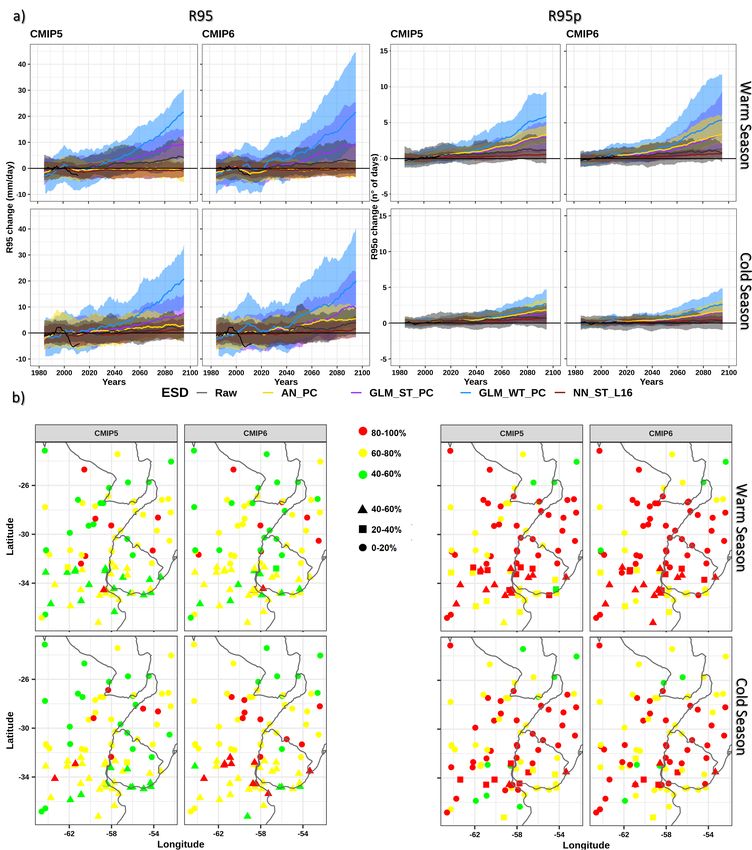
considering a set of years with the largest frequency of extreme rainfall events for assessing model
capability in simulating a wetter climate. Here, we propose to apply some of those ESD techniques to a
set of GCMs runs during their historical and future periods. Thereby, the main objectives of the present
work are to generate a multi-model ensemble of statistically downscaled GCMs outputs of daily
precipitation over SESA and to assess model performance and uncertainty in the historical and future
periods, with special focus on extreme precipitation.

2. Data And Methodology
2.1 Observational data:

Daily precipitation records from 86 meteorological stations over SESA were considered during the period
1979-2017 (Figure 1a), which have been used and quality-controlled in previous studies by the research
group (Olmo and Bettolli, 2021b). These records were provided by the National Weather Services of
Argentina, Brazil, Paraguay and Uruguay and the National Institute of Agricultural Technology of
Argentina and presented less than 20% of missing data.

2.2 ESD:

a) Data

Based on the evaluation of multiple cross-validated ESD models performed by Olmo and Bettolli (2021b),
the present experiment selected specific models from this previous work following the perfect-prognosis
approach, which considers reanalysis predictors as quasi-observations to train the statistical models
(Maraun et al. 2015). ESD models were trained during the observational period 1979-2017 using ERA-
Interim daily mean fields (Dee et al. 2011) of the following variables interpolated at 2° grid resolution over
50-67°W and 20-40°S (blue box in Figure 1a): geopotential height at 500 and 1000 hPa (Z500 and Z1000,
respectively); meridional wind at 850 hPa (V850); specific humidity at 700 and 850 hPa (Q700 and Q850,
respectively) and air temperature at 700 and 850 hPa (T700 and T850, respectively). The choice of
predictors was proposed considering previous downscaling experiments and the evaluation of the
synoptic environment associated with extreme precipitation over SESA (Rasmussen and Houze 2016;
Bettolli and Penalba 2018; Olmo and Bettolli 2021a). Thus, the predictor sets used in this work involved
different configurations with pointwise predictors - using the values from the four and sixteen nearest grid
points to the target station point - and spatial-wide predictors information by using the principal
components (PCs) - explaining 95% of the total variance (Table 1). The first approach was considered to
address local influences, whereas the last one was used to retain the large-scale atmospheric structures.
Although a detailed description of the application of the ESD models will be given in the following lines,
the reader is referred to Olmo and Bettolli (2021b) for a comprehensive evaluation of the calibrated
models selected for the present work.

                                                  Page 4/30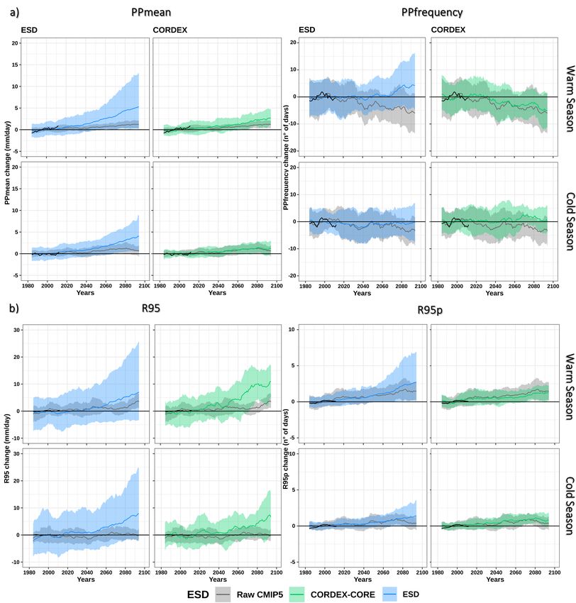
Simulations from 12 GCMs from the CMIP5 and CMIP6 experiments (Taylor et al. 2012; Eyring et al.
2016) were used in the application of the ESD models. These sets of models were selected since they
have full availability for the different predictor variables and levels, including the Andes mountain range.
Historical outputs of the predictor variables mentioned above during the period 1979-2005 (1979-2014)
were considered for the CMIP5 (CMIP6) models. Furthermore, in order to obtain downscaled climate
projections for the 21st century, future model outputs covering the period 2006-2100 (2015-2100) from
the RCP8.5 (SSP585) simulations were employed. Although these two future scenarios are not strictly
comparable, both imply the worst-case scenario in each CMIP experiment. GCMs predictor variables were
interpolated to a common grid of 2°. Additionally, raw precipitation outputs from the GCMs in their native
grid resolution - selecting the closest model grid cell to each station point - were included in the different
analyses for comparative purposes. A complete description of the GCMs used in this study is presented
in Table 2.

b) Methods

In order to produce a large multi-model ensemble of statistically downscaled GCMs, different families of
ESD models were considered in the present work:

    Analogs

The analog method (AN, Zorita and von Storch 1999) consists of finding, for each daily record, the most
similar large-scale atmospheric configuration (the nearest neighbour) in the rest of the period to obtain
the local prediction according to a similarity metric (in this case, the Euclidean distance). The ANs have
been widely applied in different regions due to its simplicity and ability to account for the non-linearity of
the predictor-predictand relationships (Timbal et al. 2009; Bettolli and Penalba 2018; Gutiérrez et al.
2019). The main drawback of this technique is that the catalog of analog days is constrained to the
observed period and therefore it cannot predict values outside the observed range. This makes the ANs
sensible to possible non-stationarities in a climate change scenario, which should be cautiously
considered (Benestad, 2010).

    Generalized Linear Models

The generalized linear models (GLMs) are an extension of linear regression in which the predictand
variable can belong to a non-linear distribution. Given that in this work special attention is taken in
extreme precipitation, stochastic versions of the GLM were adopted, considering a random sample from
the predicted distribution at each time step (GLM_STs). As performed by Olmo and Bettolli (2021b), these
models consisted in a two-stage implementation, with a Bernoulli distribution and a logit link for
precipitation occurrence, and a Gamma distribution and log link for precipitation amounts (San Martin et
al. 2017; Bedia et al. 2020). Hence, two simulated time-series were produced at each station point so that

                                                   Page 5/30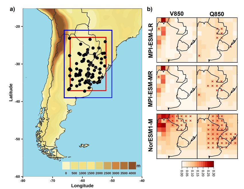
the final rainfall time-series was calculated by multiplying these two series (see Bedia et al. (2020) for
further details).

    Generalized Linear Models + Weather Types

This family of ESD models is made up of circulation-conditioned GLMs (GLM_WTs) (San Martin et al.
2017; Olmo and Bettolli 2021a). The classification of 16 weather types (WT), found in Olmo and Bettolli
(2021a) based on Z500 anomalies over southern South America, was used to calibrate the GLM
individually for each WT. Note that these are deterministic GLMs, thus, the precipitation occurrence is
obtained by transforming the simulated probability values into binary ones considering the climatological
probability of rain as threshold, whereas precipitation amounts are the expected values modelled by
optimizing the conditional mean. For this method, the Z500 daily anomalies of the GCMs were projected
into the ERA-Interim weather types according to the Euclidean distance.

    Neural Networks

The artificial neural networks (NNs) are non-linear regression-based models made of a chain of neurons
organized in layers of feed-forward networks. The model structure relies on these neurons being
connected between consecutive layers from the input layer - daily predictors fields - through a set of
hidden layers in the network, to the output layer. These connections are characterized by different weights
- that the network optimize from the input data - and activation functions, which are non-linear functions
applied in each neuron (Cavazos, 1999; Haylock et al., 2006; Vu et al. 2015; Baño-Medina et al., 2020;
Baño-Medina et al., 2021). Following the model construction employed in Olmo and Bettolli (2021b), a
two-layers NN configuration with 25 and 15 neurons, respectively, was selected. The learning rate
parameter was set to 0.01 and the activation function in the hidden layers was the sigmoid function.
Similarly to the GLMs, a stochastic set-up of NNs (NN_ST) was included in this study, which was
implemented in two stages: one for precipitation occurrence - for which the output layer performed a
linear function - and one for precipitation amounts, for which the output layer performed the sigmoid
function. Following the recommendations by Baño-Medina et al. (2020), the NN optimizes the negative
log-likelihood of a Bernoulli-Gamma distribution. Specifically, it estimates the rain probability from the
Bernoulli distribution and the shape and scale parameters of the Gamma distribution to obtain the rain
occurrences and amounts, respectively.

Note that deterministic GLM and NN simulations of daily precipitation were previously analyzed, resulting
in systematic underestimations of precipitation amounts - particularly in extremes - and generally
presented poorer performances than their stochastic versions or other ESD families. Hence, this work will
be centered on the application of the ESD techniques that best represented the main features of daily
precipitation as shown by Olmo and Bettolli (2021b). For each ESD model family (AN, GLM_ST, GLM_WT
and NN_ST), two models with different predictors configuration were chosen based on their performance
in the cross-validation procedure (Olmo and Bettolli 2021b). In this way, in the present study 8 ESD
models - outlined in Table 1 - were applied to the GCMs outputs for their historical and future periods. The
ESD methods were implemented using the R-based climate4R open framework (Bedia et al. 2020).
                                                  Page 6/30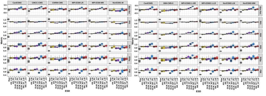
c) Evaluation framework

The perfect prognosis approach assumes that GCMs are able to adequately reproduce the predictors as
depicted by the reanalysis dataset. For this reason, the distributional similarity between the representation
of predictor variables by the GCMs and ERA-Interim was addressed here by performing a two-sample
Kolmogorov-Smirnov (KS) test, which is a non-parametric test for checking the null hypothesis that two
datasets come from the same distribution. The KS statistic presents values from 0 to 1, where the lowest
values indicate greater distributional similarity. Following the methodology suggested by Bedia et al.
(2020), standardized anomalies of the predictor variables were compared using an effective sample size
due to the strong serial correlation on the daily time-series, at the 99% level of confidence.

Regarding the precipitation simulations, statistically downscaled GCMs were evaluated separately
according to the CMIP version of each GCM, that is, model analysis was carried out for their respective
historic and future periods individually (Table 2). The meteorological station points over SESA were used
as reference. On one hand, multiple validation indices adapted from the VALUE intercomparison
experiment (Maraun et al. 2015) were estimated during the historical period, encompassing the main
features of daily precipitation. The indices are the relative bias (Bias Rel.), the frequency of rainy days
(R01), the precipitation intensity (as depicted by the simple precipitation intensity index, SDII), the
intensity and frequency of days with precipitation above 20 mm (R20 and R20p, respectively) and the
98th percentile of the daily precipitation distribution in wet days (P98). In all cases (observations and
models), the threshold for a rainy day was set at 1 mm per day. On the other hand, the spatio-temporal
variability of precipitation extremes was assessed by analyzing their spatial behaviour, intensity and
intra-annual variability. To this end, extreme rainfall was defined at each station point as the precipitation
values in those days when the accumulated precipitation exceeded the 95th percentile (P95) of the
empirical distribution of rainy days. This daily percentile was calculated in the base period 1986-2005,
considering a 29-days moving window centered on each calendar day. In addition, Taylor diagrams
(Taylor, 2001) were illustrated for summarizing the representation of the spatial patterns of precipitation
over SESA. These diagrams quantify the degree of statistical similarity between the stations reference
dataset and the models, reporting the Pearson correlation coefficient, the standard deviation and the
centered root mean squared error.

For the analysis of the downscaled projections, anomalies from the 1986-2005 base period were
estimated in each model output and time-series of specific precipitation indices were constructed using
both historical and future simulations. The indices used here were chosen to study changes in both the
intensity and frequency of rainy days (PPmean and PPfrequency, respectively) and precipitation extremes
based on the estimation of the P95 as described above (R95 and R95p for extremes intensity and
frequency, respectively). Moreover, agreement maps showing the coincidence among the multi-model
ensemble in the projected changes were plotted over SESA.

                                                   Page 7/30
2.3 RCMs
In order to inter-compare the statistically downscaled projections obtained here with other dynamical
downscaling models, the regional climate models RegCM4v7 and REMO2015 from the CORDEX-CORE
initiative (Gutowski et al. 2016) were considered. Particularly, daily RCMs precipitation from the historical
(1979-2005) and RCP8.5 (2006-2100) experiments driven by three CMIP5 GCMs were employed (MPI-
ESM-LR, MPI-ESM-MR and NorESM1-M). Note that these three GCMs were also used for the ESD
simulations in the present work (Table 2). In this way, 4 simulations were compared with the different
statistical downscaling outputs of the common GCMs: MPI-ESM-MR_RegCM4v7, NorESM1-
M_RegCM4v7, MPI-ESM-LR_REMO2015 and NorESM1-M_REMO2015. A more detailed description of the
RCMs simulations is displayed in Table 3. Even though the validation of these RCMs is beyond the scope
of this study, they have already been evaluated and used over the region in the literature and their skills
and shortcomings were identified (Olmo and Bettolli 2021a; Teichmann et al. 2020). Thereby, the focus of
this analysis will be on the comparison of the variety of downscaled projections in terms of model
agreement and spread in the intensity of changes over SESA.
3. Results
3.1 Historical evaluation
For the perfect prognosis assessment, KS score maps for V850 and Q850 in three of the GCMs listed in
Table 2 are illustrated in Fig. 1b (results of the rest of the GCMs and predictor variables are available in
Figure S1 as supplementary material). Distributional similarity varied among GCMs, although the larger
discrepancies in the representation of Q850 and Q700 were consistent in many of the models. The
differences between ERA-Interim and some GCMs distributions were significant over the center and
northeastern parts of the domain for Q850 and Q700, respectively, thus limiting at some point the
validation of the perfect prognosis hypothesis in some areas. For instance, the NorESM1-M model
seemed to present significant differences more spatially extended than the rest of the GCMs. It is
interesting to highlight that, in the case of Q850, the different MPI models tended to show more
agreement with ERA-Interim than the rest of the models. Despite this regular performance of the GCMs in
appropriately representing specific humidity, moisture-related variables are crucial predictors when
simulating precipitation, which is the reason why it was included in the different predictor sets. The rest
of the predictor variables were generally well represented by the GCMs, while V850 exhibited more
differences in the grid cells near the Andes mountain range, but were not significant (Fig. 1b and Figure
S1 of the supplementary material). These outcomes become useful information for the interpretation of
the downscaled results and exhibit the difficulty of some GCMs in representing specific humidity over
SESA.
Page 8/30An initial inspection of the statistically downscaled GCMs was carried out by analyzing the performance
in the indices described in Sect. 2.2. Boxplots in Fig. 2 present, for each GCM, the estimated indices in
every station point over SESA, and the first box presents the comparison with the raw GCM precipitation
data (CMIP5 and CMIP6 models are displayed in Figs. 2a and 2b, respectively). In terms of model biases,
the different ESD families satisfactorily reduced the model biases. The exception were the GLM_WTs,
especially the GLM_WT_PC configuration, which often presented wet biases (for instance, in the
CanESM2 and CMCC-CMS CMIP5 models and in the CanESM5 and MPI-ESM2-1-HR CMIP6 model). Most
of the ESD models showed added value to the raw GCM precipitation, as depicted by the boxes nearer to
the zero line. This was consistent when applied to almost all the GCMs, although the CMIP5 NorESM1-M
model (Fig. 2a) presented dry biases in all the ESD models like the raw GCM values. When analyzing the
frequency of rainy days (R01), all ESD models reduced the magnitude of the differences found in the raw
GCM precipitation and exhibited smaller spatial spread as reflected by smaller boxes. GCMs generally
overestimate rain frequency, especially at low values (Bador et al. 2020), which was alleviated by the
statistical downscaling procedure. In the case of precipitation intensity (SDII), the ESD models again
outperformed the raw GCM data, particularly the ANs and NN_STs, which presented SDII ratios near zero.
The GLM_STs and GLM_WTs tended to overestimate the index, more pronounced in GLM_WT_PC. This
behaviour of the different ESD models was coincident in all the GCMs from both CMIP experiments
(Figs. 2a and 2b).
Regarding the indices related to heavy precipitation, the ESD models were able to reproduce R20 and
R20p when applied to most of the GCMs. The GLM_WTs presented the largest differences, but no general
behaviour could be summarized as their performance often varied among GCMs. As mentioned above,
ESD performance in NorESM1-M was weaker than in the other GCMs, as all the ESD models tended to
underestimate the indices, although this was less intense than in the raw GCM (Fig. 2a). The analysis of
extreme precipitation as depicted by the P98 index exhibited the strongest underestimations in the raw
GCMs (Fig. 2a and 2b, last row). These models were not able to successfully represent intense rainfall as
this phenomenon is associated with sub-grid processes - at regional and local scales - that the GCMs
cannot reproduce. In this sense, applying different downscaling tools to these models arises as a
necessary procedure for a better representation of precipitation extremes. The majority of the ESD models
used in this work exhibited a clear added value in the P98 index. The ANs presented a reduced spatial
spread and were always positioned on the zero line, while the stochastic models (GLM_STs and NN_STs)
also exhibited a good performance but little overestimating heavy precipitation intensities. The GLM_WTs
tended to underestimate the index, especially GLM_WT_L4, which performed similarly to the raw GCM
data. This GLM_WT only considers local predictors, which may be misrepresented by the GCMs (Fig. 1b).
Furthermore, the circulation-conditioned GLMs are deterministic models and therefore they are
constructed to reproduce the conditional mean, which may cause the models to underestimate heavy
precipitation.
In this context, results from the statistically downscaled GCMs with the ESD models used here are in line
with previous findings for these statistical models when considering a cross-validation procedure (Olmo
and Bettolli, 2021b), indicating that the models could extrapolate the predictor-predictand relationships
Page 9/30learnt from the reanalysis to the GCM predictors data and thereby were able to improve their reproduction
of daily precipitation in the historical period, particularly in extremes.
In a following analysis, the spatial patterns of mean and extreme precipitation over SESA were studied
through Taylor diagrams (Fig. 3). The diagrams were plotted separately for each CMIP and for the warm
and cold austral seasons (from October to March and from April to September, respectively). The
different ESD families were illustrated with different colours and the raw GCM precipitation was included
for comparative purposes (considering the nearest model grid cell to each station point). A first insight
into these diagrams pointed out that the ESD models presented larger spatial variability - in terms of the
standard deviation - than the raw GCM data, closer to the observations. Note that this is expected at some
point since raw GCMs are employed using the nearest model grid cells, which may cause some raw
values to be repeated and therefore leading to an underestimation of the spatial variability.
Notwithstanding, the ESD techniques produce regional-to-local scale information with higher spatial
resolution. The ANs and GLM_STs were the most accurate ESD families in representing the spatial
patterns of PPmean and P95, indicated by high correlations and standard deviations generally near one.
Furthermore, the configurations with spatial predictors - by considering the principal components of the
predictors set - exhibited the best performances (AN_PC and GLM_ST_PC), which is in agreement with
results from Olmo and Bettolli (2021b) when driven by ERA-Interim reanalysis. These features were
observed for both seasons, CMIP and mean fields (PPmean and P95). The NN_STs tended to
overestimate the spatial variability of these patterns particularly during the warm season (standard
deviation above one in most of the cases), although they presented small dispersion among the different
predictor configurations and GCMs. The GLM_WTs usually exhibited a larger cloud of points, however, the
performance of the GLM_WTs ensembles (indicated with squares) was like the other ESD families in
mean precipitation.
When comparing both seasons of the year, the warm season was typically more problematic to be
simulated by the different models, exhibiting a larger model spread more pronounced for P95. This
spread seemed to be reduced in each ESD family for the CMIP6 models compared to the CMIP5 GCMs.
The warm season presents a marked SW-NE gradient with large amounts of precipitation, and extreme
rainfall events during this season are the main contributors to the total annual accumulated precipitation
(Cavalcanti et al. 2015). Thus, this is a challenging spatial structure for the downscaled GCMs, as
reflected by the lower spatial correlations and larger differences in the standard deviations in P95 than in
PPmean. Nonetheless, they adequately simulated this feature of precipitation extremes in most of the
cases, better than the raw GCMs. It is worth mentioning that results from NorESM1-M (numbered 6 in the
CMIP5 panels of Fig. 3) usually distinguished from each ESD family cloud with lower correlations and/or
larger overestimations of the standard deviation. This is in line with the model performance and
shortcomings in the indices described above (Fig. 2a) and could be related to the misrepresentation of
specific humidity identified in the perfect prognosis assessment (Fig. 1b).
In order to evaluate the intra-annual variability of extreme precipitation over SESA, the regional averaged
annual cycles of P95 were displayed in Fig. 4. It was notable the clear improvement in the representation
Page 10/30of P95 not only in its intensity but also in the shape of the annual cycle when comparing the statistically
downscaled GCMs with the raw GCM data (grey lines). This added value was congruent in almost all the
ESD models, except for GLM_WT_L4 that - even though it managed to capture the shape of the cycle -
systematically underestimated extreme intensities throughout the year, especially during the warm
season. Note that GLM_WT_PC exhibited different performances depending on the driver GCM, as
reflected by the poor representation of the annual cycle when using MPI-ESM2-1-HR and the
overestimation of its amplitude in NorESM2-MM. The rest of the ESD models satisfactorily represented
the cycle, with the AN models presenting the best performances and the stochastic models often
overestimating extreme intensities. This overestimation varied in the different GCMs as it was detected
during the austral summer, for instance, in the CanESM2 and CanESM5, whereas more clear
overestimations were found during winter in some GCMs like MPI-ESM2-1-HR and NorESM2-MM.
Nevertheless, the statistically downscaled GCMs outperformed the raw GCMs, which failed in reproducing
the intensity and the intra-annual variation of extreme rainfall over SESA, pointing out again the necessity
of a downscaling procedure to perform climate studies of spatio-temporal variability of extreme
precipitation.
3.2 Future projections
A general outcome of the evaluation of the statistically downscaled GCMs during the historical period
(Sect. 3.1) is that most of the ESD models presented added value in most of the metrics and
assessments performed here. The strengths and limitations of the different statistical models were
identified, allowing us to continue the analysis of the future projections in a subset of ESD models that
were the most accurate during the present climate. Based on these results, in the following analyses one
model configuration for each ESD family will be considered. The models AN_PC, GLM_ST_PC,
GLM_WT_PC and NN_ST_L16 will be used hereafter in the construction of a multi-model ensemble of
downscaled projections.
Figure 5a displays the time-series for mean precipitation changes in terms of the intensity and frequency
of rainy days. Changes from the 1986–2005 reference period were calculated for each model and the
different ESD families’ ensembles were illustrated together with the raw GCMs ensemble for both CMIP5
and CMIP6, separately. In mean precipitation (PPmean), greater increases were generally detected in the
warm season than in the cold season. The statistically downscaled projections showed intensified
positive changes compared to the raw GCM outputs, although their intensity and model spread notably
varied among ESD families. The NNs exhibited a reduced spread in the ensemble and showed positive
changes like the raw GCMs. Greater intensifications in mean precipitation were detected by the ANs and
GLM_STs, with the latter presenting a larger spread especially by the end of the 21st century. The largest
uncertainty was observed in the GLM_WT_PC projections, as these models depicted the greatest changes
and differences among the ensemble, particularly during the warm season. When comparing the CMIP5
and CMIP6 downscaled simulations, greater anomalies were reached in the latter set of models, although
this was associated with a larger model spread in the GLMs.
Page 11/30In the case of the frequency of rainy days (PPfrequency) (Fig. 5a, right panels), no clear sign of change
was found as most of the simulations (ESD and raw GCMs) exhibited fluctuations on the zero anomalies
line, particularly in the cold season. Note that raw CMIP5 and CMIP6 changes presented opposite signs at
the end of the century during the warm season. Among the ESD simulations, the ANs differed from the
rest of the statistical models as they started to present larger increases in PPfrequency around 2040, with
more discrepancies among the ensemble.
In fact, the performance of the different ESD methods varied among GCMs as displayed in Figure S2 (see
supplementary material), where the individual downscaled and raw GCM time-series were illustrated. This
analysis exposed that the spread and intensification of PPmean changes in the GLM_ST_PC and
GLM_WT_PC ensembles was related with specific GCMs, like CanESM2 and CanESM5, whereas in other
GCMs the behaviour of these ESD families was in better agreement with the other statistical models. In
addition, the increasing PPfrequency simulated by the ANs was more intense, for instance, in the
CanESM2, MPI-ESM-LR, CanESM5 and MPI-ESM2-1-LR models. Therefore, the sensibility of the ESD
methods to the driver GCM should be cautiously considered in the evaluation of plausible climate change
scenarios over SESA.
Figure 5b presents the agreement among ESD simulations in the changes during the 2071–2100 period
in terms of the percentage of ESD models that coincided in the sign of the changes (colours) and the
percentage of ESD models that surpassed the observed variance of the time-series (symbols). Most of
the models agreed in the sign of PPmean changes (left panels), with percentages between 80–100% in
the center of SESA. Model agreement in PPfrequency changes (right panels) was lower especially in the
cold season - up to 40% in all the stations - whereas the agreement was stronger during the warm season
in central SESA. Note, however, that these changes were not larger than the observed variance of this
index in most of the ESD simulations, which was consistent with the analysis of the time-series in Fig. 5a.
When analyzing the projections in extremes (Fig. 6), general increases in their intensity (R95) and
frequency (R95p) were detected in the different simulations. Nevertheless, in coincidence with the results
of mean precipitation described above, the rates of change varied among them. Raw GCMs exhibited
increases in the intensity of extreme rainfall during both seasons from the mid-21st century in CMIP5 and
CMIP6 datasets. This was similarly reproduced by the ANs and NN_STs in the cold season, whereas in
the warm season they were near zero throughout the 21st century. The GLM_STs presented greater
changes, although with larger spread in the ensemble. In the case of the GLM_WTs, they exhibited large
uncertainty as they differed in the intensity of the changes projected by the end of the century with the
rest of the simulations and presented important discrepancies among the ensemble.
The positive changes in the frequency of extreme precipitation events (R95p, right panels in Fig. 6a) were
coincident in the different model outputs and more pronounced during the warm season. The ANs and
GLM_STs performed similarly, although a larger spread was found in the latter. The neural networks
exhibited the smallest changes and the ensemble mean showed changes even lower than the raw GCMs.
Again, the rates of change were the greatest in the GLM_WTs, with large uncertainty in their ensemble. As
Page 12/30observed for PPmean (Fig. 5a), model spread during the warm season was larger in CMIP6 than in CMIP5
downscaled models. When analyzing the individual GCMs time-series (see Figure S3 in a supplementary
material), it was found that the large intensification of the R95 projected changes by GLM_WT_PC was
consistent in all downscaled GCMs, whereas changes in R95p presented more differences among GCMs,
in agreement with results of mean precipitation (Figure S2). On the other hand, the GLM_STs exhibited
greater R95 changes than other models only in a few GCMs like CanESM5 but affecting the ensemble
anyway.
In terms of model agreement by the end of the century (2071–2100) (Fig. 6b), changes in R95p were
more consistent among ESD models than in R95. This was depicted by the percentage of models that
agreed in the sign of the R95p changes - which was between 80–100% over most of SESA (red symbols) -
whereas these values for R95 were generally between 40–80%. In terms of change rates, around 20 and
up to 60% of the simulations surpassed the observed variance of both indices over southern SESA
(squares and triangles), indicating larger confidence in the changes over these areas.
The increases detected in mean and extreme precipitation over SESA agree with previous studies
considering outputs from RCMs using driver GCMs from CMIP5 (Blázquez and Solman, 2020; Teichmann
et al. 2020). Nevertheless, this climate change signal can be intensified or weakened by the combination
of the ESD and GCMs considered. In particular, the intensification of the projected changes by the GLM
models was previously detected by Baño-Medina et al. (2020) when applied to one GCM for different
temperature and precipitation daily metrics in Europe. Notwithstanding, our results over SESA expose that
these statistical models behave differently in the stochastic and in the circulation-conditioned versions,
being the latter the one that exhibited the largest uncertainty.
3.3 Intercomparison with RCMs
As discussed in the literature, extreme precipitation events over SESA are strongly controlled by regional
forcings, which are generally better captured by the RCMs than the GCMs (Blázquez and Solman, 2020;
Falco et al. 2019). Hence, it is likely that the climate change signal is not always consistent between
them, so the downscaled projections become more reliable in terms of the changes in extreme
precipitation. As described in Sect. 3.2, the statistical models can also modify the GCM signal of change,
although this result clearly depends on the ESD method and the choice of GCM. In this sense, it becomes
interesting to evaluate if the ESD models depict climate projections congruent with the RCMs and to
inspect their differences in the multiple precipitation indices analyzed in Sect. 3.2.
Regional time-series of the mean and extreme precipitation indices previously assessed are displayed for
the ESD and CORDEX ensembles in Fig. 7 (a and b, respectively). For each ensemble, only the simulations
with the 3 CMIP5 GCMs in common between the ESD and CORDEX-CORE RCM models were considered
(Table 3). Raw GCMs ensemble was also illustrated in grey tones. Note that, for this comparison, the ESD
ensemble presents a greater number of members than the CORDEX ensemble (12 versus 4 simulations).
Page 13/30In terms of mean precipitation intensities (PPmean, left panels in Fig. 7a), the ESD ensemble presented
larger spread and more intense positive changes by the end of the century than the CORDEX ensemble -
especially during the warm season - which was mainly due to the inclusion of the GLM_WTs. On the other
hand, PPfrequency showed different behaviours in both seasons of the year. Raw GCMs projections for
the warm season showed a decline in the frequency of rainy days, which was reproduced by the CORDEX
ensemble. In contrast, the ESD models presented no clear changes until around 2060, when positive
anomalies started to emerge. This was particularly due to the analog models (see Figure S2). During the
cold season, the ESD ensemble behaved similarly to the raw GCMs in both ensemble mean and spread,
presenting some differences by the end of the century. The CORDEX ensemble exhibited more differences
from the raw GCMs and showed positive anomalies in its mean. Despite these particularities, both
downscaled sets of simulations showed no clear changes for PPfrequency during the cold season.
In the case of extreme indices (Fig. 7b), the spread in both downscaled sets was larger in R95 than in
R95p, particularly in the ESD ensemble. However, the ensemble means were congruent in both seasons,
expecting an increase in extreme rainfall intensities by the end of the century. The frequency of extreme
events is projected to increase according to both statistical and dynamical downscaling models, which
was in good agreement with the climate change signal from raw GCMs. The ESD models closely followed
the GCMs ensemble until around 2070, when more intense changes predominated in the ensemble. As
observed in Figure S3, this was due to GLM_WT_PC, that amplifies the climate change signal when
applied to MPI-ESM-LR and MPI-ESM-MR, whereas the simulations for NorESM1-M were in accordance
with the other downscaled simulations.
4. Discussion And Conclusions
The present study is centered over southeastern South America (SESA), a region that stands out in terms
of the frequency and intensity of extreme precipitation events, which have strong impacts on the socio-
economic activities of the region. Thus, high-resolution climate information is required for impact studies
such as hydrological modelling and for the evaluation of possible future scenarios in a context of global
warming. Thereby, the focus of this work is on the construction of a multi-model ensemble of statistically
downscaled GCMs, considering different empirical statistical downscaling (ESD) techniques and a variety
of CMIP5 and CMIP6 models. The ESD models were calibrated using ERA-Interim predictors and daily
precipitation records from a meteorological stations network over SESA during 1979–2017 and then
applied to the sets of GCMs. These models included analogs (ANs), generalized linear models in
stochastic and circulation-conditioned versions (GLM_STs and GLM_WTs, respectively) and stochastic
neural networks (NN_STs), following the experiment from Olmo and Bettolli (2021b).
The downscaled models showed added value for most of the GCMs in several aspects such as the
relative bias and intensity and frequency of rain, but particularly in heavy and extreme intensities, where
raw GCMs exhibited strong underestimations (Fig. 2). In terms of spatial variability, the evaluation of the
mean and extreme precipitation spatial patterns through Taylor diagrams allowed us to distinguish the
performance of the different ESD families, being the ANs and GLM_STs the most accurate, especially in
Page 14/30configurations with spatial predictors by considering the principal components (Fig. 3). ESD model
performance was better in mean than in extreme precipitation (defined by the 95th percentile, P95),
especially during the warm season, when extreme events highly contribute to the total precipitation
amounts (Olmo and Bettolli, 2021a). When studying the intra-annual variability of extreme rainfall - in
terms of the annual cycle of P95 in Fig. 4 - the added value of most ESD models was clear and consistent
in all GCMs. Some GLM_WT models exhibited more difficulties in reproducing the shape of the annual
cycle and tended to underestimate extreme intensities, although their performance was usually better
than the raw GCMs, which were not able to capture neither the intensities nor the shape of the cycle,
pointing out the necessity of performing a downscaling procedure.
Future projections of mean and extreme precipitation from the multi-model ensemble of statistically
downscaled GCMs were summarized in regional averaged time-series and model agreement maps
(Figs. 5 and 6). ESD projections showed intensified positive changes in mean precipitation compared to
the raw GCMs - like in the case of the ANs and GLM_STs - even though the intensity of these changes and
model spread notably varied between ESD families (Fig. 5a). The circulation-conditioned GLMs
(GLM_WTs) presented large uncertainty as depicted by distinguished change rates and ensemble spread,
particularly during the warm season. The frequency of rainy days did not evidence a clear sign of change,
although ESD simulations presented an increment during the warm season - more pronounced in the ANs
- in agreement with CMIP6 raw models but contrary to the CMIP5 set. In the case of extreme precipitation
(Fig. 6a), increases in the intensity (R95) and frequency (R95p) were generally detected, even though the
change rates varied among simulations. Model agreement was greater for R95p as depicted by the
percentage of models that agreed in the sign of the changes, which generally surpassed the observed
variance of the index, indicating larger confidence over southern SESA (Fig. 6b). As for mean
precipitation, the GLM_WTs exhibited notably larger spread and intensification than other ESD families,
while the NN_STs tended to present changes similarly to raw GCMs.
It is important to highlight that the behaviour of the different ESD methods varied among GCMs, as seen
in the individual GCM time-series (see Figure S2 and S3 in a supplementary material). In addition, even
though an optimal outcome from any downscaling procedure would be the reduction of model spread
and uncertainty compared to the raw GCM outputs, the intensity of precipitation changes - and
particularly in extreme events - expected during the 21st century presented dispersion among the multi-
model ensemble of ESD simulations. This was often larger than the one detected in the raw GCM data,
although most of them agreed on the sign of the changes. Note, however, that multiple ESD techniques
and different GCMs were employed in the generation of the downscaled projections, which may introduce
large differences among the simulations, intensifying the ensemble spread. Notwithstanding, all ESD
models seemed to be coincident until the middle 21st century, when a clear dispersion starts to emerge
among the ensembles. In this way, the larger spread and/or intensification of changes in some
precipitation indices was often related to specific GCMs but affecting the ESD ensemble anyway. This
was mainly due to the inclusion of GLM_WT. The reasons behind this behaviour could be different
representations of the circulation patterns by the GCMs, their changing frequency and the within-type
variability, related to the stationarity assumption on the relationship between WTs and the surface
Page 15/30variable (Cahynová and Huth, 2016). The analysis of the weather types evolution and representation by
the GCMs is beyond the scope of this work, however, it implies an essential task to understand the
GLM_WTs behaviour and sensibility, particularly from the middle and late 21st century. This topic will be
addressed in future studies.
Finally, given that extreme precipitation events are strongly controlled by regional forcings, it is expected
that the climate change signal presents discrepancies between raw GCMs and downscaled models, as
the latter simulations better reproduce the main features of heavy rainfall. In this sense, to compare the
statistically downscaled projections with other downscaled simulations available for the region, the
CORDEX-CORE RCM simulations for the South American domain were analyzed. The ESD ensemble
presented larger spread and more intense positive changes in mean precipitation than the CORDEX
ensemble, especially during the warm season (Fig. 7a). For extreme indices, both downscaled sets of
models agreed on the increase signal for extreme intensities by the end of the century. These ensembles
projected increments in R95p in congruence with raw GCMs, while the ESD ensemble started to present
more differences only by the end of the century.
As explained before, the ESD ensemble exhibited a larger spread than the CORDEX RCMs ensemble,
although this spread was intensified due to the GLM_WTs. In coincidence, San Martin et al. (2017)
evaluated future precipitation projections over Europe by statistical and dynamical downscaling
ensembles and found a larger spread in the ESD simulations, while ESD models’ dispersion was
dominated by the choice of GCM rather than by the choice of ESD model family. This last result was also
found in the evaluation of the future ESD projections over SESA (Sect. 3.2), which evidences the
complexity of performing a downscaling procedure and the assessment of possible future expectations,
particularly when it comes to intense rainfall, which should be cautiously considered in the evaluation of
plausible climate change scenarios over SESA.
It is worthwhile mentioning that NorESM1-M downscaled simulations typically showed lower scores in
the different metrics and evaluations during the historical period compared to the rest of the GCMs, such
as in extreme intensities indices in Fig. 2 and in the spatial patterns as depicted by Taylor diagrams.
These shortcomings could be associated with its limitations in the representation of predictor variables,
in particular, specific humidity at 850 hPa (Fig. 1), thus limiting the compliance of the perfect prognosis in
the ESD experiment. However, this GCM was included in the analyses since it is one of the few GCMs
used to nest the CORDEX-CORE RCMs in the South American domain. Furthermore, although in this study
an unprecedented number of GCMs was employed in the statistical downscaling procedure over SESA (6
CMIP5 and 6 CMIP6 models), this is still not enough to present robust conclusions on the performance
and comparison of each CMIP experiment. Nonetheless, no particular behaviour was identified in each
set of GCMs. Only a more reduced model spread could be found in CMIP6 in the evaluation of the spatial
patterns of mean and extreme precipitation over SESA, while the spread in the projections was associated
with the choice of ESD family and often on specific GCMs.
Page 16/30Overall, this is a novel work that moves forward on the application of statistical downscaling methods to
assess climate changes over SESA in a global warming scenario, detecting the strengths and
shortcomings of different techniques, particularly in extreme precipitation. Further research needs to be
done in order to assess whether statistical downscaling can generate plausible climate change scenarios
and to reduce model uncertainty, even though a general clear message was found among downscaled
projections in terms of the agreement in increased mean precipitation and frequency of extreme events
over the region. This agreement was consistent until the middle 21st century when model spread started
to increase. Particularly, a more comprehensive evaluation of the stationarity assumption in the statistical
downscaling of future GCM simulations needs to be performed (Vrac et al. 2007), which will be the focus
of a follow-up study. In this sense, these results should be cautiously interpreted, although this work
reveals that the developed statistical models are able to bridge the gap between coarse-resolution GCM
data and regional-to-local scale features and are promising for studying precipitation extremes in a
changing climate.
Table captions
Declarations
Acknowledgments
This work was supported by the University of Buenos Aires 2018-20020170100117BA,
20020170100357BA and the ANPCyT PICT-2018-02496 and PICT 2019–02933 projects. The authors
acknowledge the WCRP CMIP5 and CMIP6 and CORDEX for producing and making available the model
outputs used in this work.
Competing interests: The authors declare no competing interests.
References
1. Almazroui M, Ashfaq M, Islam MN et al (2021) Assessment of CMIP6 Performance and Projected
Temperature and Precipitation Changes Over South America. Earth Syst Environ 5:155–183.
https://doi.org/10.1007/s41748-021-00233-6
2. Araya-Osses D, Casanueva A, Román-Figueroa C, Uribe JM, Paneque M (2020) Climate change
projections of temperature and precipitation in Chile based on statistical downscaling. Clim Dyn
54:4309–4330. https://doi.org/10.1007/s00382-020-05231-4
3. Asong ZE, Khaliq MN, Wheater HS (2016) Projected Changes in Precipitation and Temperature over
the Canadian Prairie Provinces using the Generalized Linear Model Statistical Downscaling
Approach. J Hydrol. doi:http://dx.doi.org/10.1016/j.jhydrol.2016.05.044
4. Bador M, Boé J, Terray L, Alexander LV, Baker A, Bellucci A et al (2020) Impact of higher spatial
atmospheric resolution on precipitation extremes over land in global climate models. Journal of
Geophysical Research: Atmospheres 125:e2019JD032184. https://doi.org/10.1029/2019JD032184
Page 17/305. Baño-Medina J, Manzanas R, Gutiérrez JM (2020) Configuration and Intercomparison of Deep
Learning Neural Models for Statistical Downscaling. Geosci Model Dev 13(4):2109–2124.
https://doi.org/10.5194/gmd-2019-278
6. Baño-Medina J, Manzanas R, Gutiérrez JM (2021) On the suitability of deep convolutional neural
networks for continental-wide downscaling of climate change projections. Clim Dyn.
https://doi.org/10.1007/s00382-021-05847-0
7. Bedia J, Baño-Medina J, Legasa MN, Iturbide M, Manzanas R, Herrera S, Casanueva A, San-Martín D,
Cofiño AS, Gutiérrez JM (2020) Statistical downscaling with the downscaleR package: Contribution
to the VALUE intercomparison experiment. Geosci Model Dev 13(3):1711–1735.
https://doi.org/10.5194/gmd-2019-224
8. Benestad RE (2010) Downscaling precipitation extremes: Correction of analog models through PDF
predictions, Theor. Appl Climatol 100:1–21. https://doi.org/10.1007/s00704-009-0158-1
9. Bentsen M, Bethke I, Debernard JB, Iversen T, Kirkevåg A, Seland Ø, Drange H, Roelandt C, Seierstad
IA, Hoose C, Kristjánsson JE (2013) The norwegian earth system model, noresm1-m - part 1:
description and basic evaluation of the physical climate. Geosci Model Dev 6(3):687–720. https
://doi.org/10.5194/gmd-6-687-2013
10. Bettolli ML, Solman S, da Rocha RP, Llopart M, Gutiérrez JM, Fernández J, Olmo M, Lavín-Gullón A,
Chou SC, Carneiro Rodrigues D, Coppola E, Huarte B, Barreiro R, Blázquez M, Doyle J, Feijoó M, Huth
M, Machado R, Vianna L, Cuadra S (2021) The CORDEX Flagship Pilot Study in Southeastern South
America: A comparative study of statistical and dynamical downscaling models in simulating daily
extreme precipitation events. Clim Dyn. https://doi.org/10.1007/s00382-020-05549-z
11. Bettolli ML, Penalba OC (2018) Statistical downscaling of daily precipitation and temperatures in
southern La Plata Basin. Int J Climatol 38:3705–3722. https://doi.org/10.1002/joc.5531
12. Blázquez J, Solman SA (2020) Multiscale precipitation variability and extremes over South America:
analysis of future changes from a set of CORDEX regional climate model simulations. Clim Dyn
55:2089–2106. https://doi.org/10.1007/s00382-020-05370-8
13. Cahynová M, Huth R (2016) Atmospheric circulation influence on climatic trends in Europe: an
analysis of circulation type classifications from the COST733 catalogue. Int J Climatol 36:2743–
2760
14. Cavalcanti I, Carril A, Penalba O, Grimm AM, Menéndez C, Sanchez E, Cherchi A, Sörensson A,
Robledo F, Rivera J, Pantano V, Bettolli ML, Zaninelli P, Zamboni L, Tedeschi R, Domínguez M,
Ruscica R, Flach R (2015) Precipitation extremes over La Plata Basin—review and new results from
observations and climate simulations. J Hydrol 523:211–230.
https://doi.org/10.1016/j.jhydrol.2015.01.028
15. Cavazos T (1999) Large-scale circulation anomalies conducive to extreme events and simulation of
daily rainfall in northeastern Mexico and southeastern Texas. J Clim 12:1506–1523
16. Dee DP, Uppala SM, Simmons AJ, Berrisford P, Poli P, Kobayashi S, Andrae U, Balmaseda MA,
Balsamo G, Bauer P, Bechtold P, Beljaars ACM, van de Berg L, Bidlot J, Bormann N, Delsol C, Dragani
Page 18/30You can also read