Modeling total electron content derived from radio occultation measurements by COSMIC satellites over the African region - ANGEO
←
→
Page content transcription
If your browser does not render page correctly, please read the page content below
Ann. Geophys., 38, 1203–1215, 2020
https://doi.org/10.5194/angeo-38-1203-2020
© Author(s) 2020. This work is distributed under
the Creative Commons Attribution 4.0 License.

Modeling total electron content derived from radio occultation
measurements by COSMIC satellites over the African region
Patrick Mungufeni1,2 , Sripathi Samireddipalle3 , Yenca Migoya-Orué4 , and Yong Ha Kim1
1 Department   of Astronomy and Space Science, Chungnam National University, Daejeon, South Korea
2 Physics department, Mbarara University of Science and Technology, P.O. Box 1410 Mbarara, Uganda
3 Indian Institute of Geomagnetism, New Panvel, India
4 The Abdus Salam International Centre for Theoretical Physics (ICTP) T/ICT4D, Trieste, Italy

Correspondence: Yong Ha Kim (yhkim@cnu.ac.kr)

Received: 23 November 2019 – Discussion started: 18 December 2019
Revised: 15 September 2020 – Accepted: 8 October 2020 – Published: 24 November 2020

Abstract. This study developed a model of total elec-              1   Introduction
tron content (TEC) over the African region. The TEC data
were obtained from radio occultation measurements done by
the Constellation Observing System for Meteorology, Iono-          Among the error sources that affect the positioning in the
sphere, and Climate (COSMIC) satellites. Data during geo-          Global Navigation Satellite System (GNSS) are propagation-
magnetically quiet time (Kp < 3 and Dst > −20 nT) for the          medium-related errors. In particular, the ionospheric refrac-
years 2008–2011 and 2013–2017 were binned according to             tion is the largest contributor of the user-equivalent range er-
local time, seasons, solar flux level, and geographic longi-       ror. This type of frequency-dependent error can virtually be
tude and latitude. B splines were fitted to the binned data        eliminated in dual-frequency receivers by differential tech-
to obtain model coefficients. The model was validated using        niques (Hofmann-Wellenhof et al., 2007). For the case of
actual COSMIC TEC data of the years 2012 and 2018. The             single-frequency receivers, some GNSS (e.g., Global Posi-
validation exercise revealed that approximation of observed        tioning System (GPS) and Galileo) broadcast messages in-
TEC data by our model produces a root mean square error of         clude the parameters of an ionospheric model which can
5.02 TECU (total electron content unit). Moreover, the mod-        be used to compute and correct the ionospheric effects
eled TEC data correlated highly with the observed TEC data         (Guochang, 2007). For instance, the GPS uses the Klobuchar
(r = 0.93). Due to the extensive input data and the applied        model, which represents the zenith delay as a constant value
modeling technique, we were able to reproduce well-known           at night and a half-cosine function during the day (Klobuchar,
TEC features such as local time, seasonal, solar activity cy-      1987). In the framework of the European Galileo constel-
cle, and spatial variations over the African region. Further       lation, NeQuick G based on the NeQuick model has been
validation of our model using TEC measured by ionosonde            proposed to be used for single-frequency positioning (see Is-
stations over South Africa at Hermanus, Grahamstown, and           sue 1.2, September 2016 by the European Commission, titled
Louisville revealed r values > 0.92 and root mean square er-       “European GNSS (Galileo) Open Service – Ionospheric cor-
ror (RMSE) < 5.56 TECU. These validation results imply             rection algorithm for Galileo single-frequency users”). The
that our model can estimate TEC fairly well that would be          NeQuick and its subsequent modifications (NeQuick G and
measured by ionosondes over locations which do not have            NeQuick 2) are a three-dimensional, time-dependent iono-
the instrument. Another element of the significance of this        spheric electron density model developed by the Aeronomy
study is the fact that it has shown the potential of using basis   and Radio Propagation Laboratory (ARPL) of the Abdus
spline functions for modeling ionospheric parameters such as       Salam International Center for Theoretical Physics (ICTP) in
TEC over the entire African region.                                Trieste, Italy, and the Institute for Geophysics, Astrophysics
                                                                   and Meteorology of the University of Graz, Austria (Nava
                                                                   et al., 2008). In addition to using models to reduce iono-

Published by Copernicus Publications on behalf of the European Geosciences Union.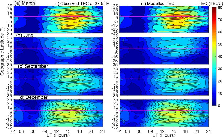
1204                                                                     P. Mungufeni et al.: Modeling total electron content

spheric refraction errors, Space Based Augmentation Sys-          lar region for which it was constructed. Opperman (2008)
tems (SBAS) such as the Wide Area Augmentation System             stated that the higher time and spatial resolution imaging
(WAAS), the European Geostationary Navigation Overlay             achievable with regional models permits the analysis of lo-
Service (EGNOS), and the GPS-aided Geo Augmented Nav-             calized ionospheric structures and dynamics not observable
igation (GAGAN) are also used (Hofmann-Wellenhof et al.,          in global models. Examples of studies that developed TEC
2007).                                                            models over some parts of Africa are the following. A neu-
   For the international standard specification of ionospheric    ral network model of GNSS – vertical TEC (GNSS-VTEC)
parameters (such as electron density, electron and ion tem-       over Nigeria was developed by Okoh et al. (2016) using
peratures, and equatorial vertical ion drift), the Committee on   all available GNSS data from the Nigerian GNSS Perma-
Space Research (COSPAR) and the International Union of            nent Network (NIGNET). An adjusted spherical harmonic-
Radio Science (URSI) recommended the International Ref-           based TEC model was developed by Opperman (2008) using
erence Ionosphere Model (IRI) (Bilitza, 2001). IRI is an em-      a network of South African dual-frequency GPS receivers.
pirical model primarily based on all available experimental       Habarulema et al. (2011) presented the Southern Africa TEC
data (ground- and space-based) sources. However, theoreti-        prediction (SATECP) model that was based on the neural net-
cal considerations have been used in bridging data gaps and       work technique. The SATECP generates TEC predictions as
for internal consistency checks (Bilitza, 2001).                  a function of input parameters, namely, local time, day of
   The ionospheric total electron content (TEC) is one of the     year, solar and magnetic activity levels, and the geographi-
important descriptive physical quantities of the ionosphere       cal location. A neural-network-based ionospheric model was
(Rama Rao et al., 1997; Ercha et al., 2012). The GNSS mea-        developed using GPS-TEC data over the East African sector
surements obtained from the global and regional networks of       by Tebabal et al. (2019). Recently, Okoh et al. (2019) used
International GNSS Service (IGS) ground receivers have be-        the neural network technique to develop a TEC model over
come a major source of TEC data. As one of the IGS analysis       the entire African region. In addition to using TEC obtained
centers, Center for Orbit Determination in Europe (CODE)          by the COSMIC RO technique, they used TEC measured by
provides Global Ionosphere Maps (GIMs) containing verti-          GPS receivers on the ground.
cal TEC data daily using the GNSS data collected from over           Due to the lack of a dense network of ground-based GNSS
200 tracking stations of IGS and other institutions. Several      receivers and poor coverage of COSMIC RO data over the
studies have used GIMs from CODE and other IGS analy-             African region, the TEC model over the entire African region
sis centers such as the Jet Propulsion Laboratory (JPL) to        presented by Okoh et al. (2019) sometimes failed to capture
construct TEC models (Jakowski et al., 2011a; Mukhtarov           the equatorial ionization anomaly (EIA) over the region. This
et al., 2013; Ercha et al., 2012; Sun et al., 2017). Jakowski     point has been illustrated with examples in Sects. 2 and 5. In
et al. (2011a) proposed the Global Neustrelitz TEC Model          this study, we applied a data binning method to the COS-
(NTCM-GL) that describes the average TEC under quiet ge-          MIC RO TEC data that allowed development of an improved
omagnetic conditions. The NTCM-GL was developed using             TEC model over the region. Moreover, we demonstrate the
GIMs during 1998–2007 provided by CODE. A global back-            potential of the basis spline functions to model TEC over the
ground TEC model was also built using CODE GIMs by                African region. These basis functions never vanish over lim-
Mukhtarov et al. (2013). The model describes the climato-         ited intervals and add up to 1 at all local times and longitudes
logical behavior of the ionosphere. The GIMs from JPL were        (De-Boor, 1978). Moreover, according to Scherliess and Fe-
used by Ercha et al. (2012) to construct a global ionosphere      jer (1999), they are ideally suited to model the equatorial
model using the empirical orthogonal function (EOF) anal-         ionosphere, which exhibits smooth and rapid changes during
ysis method. The Taiwan Ionosphere Group for Education            daytime and near sunset, respectively, by proper placement
and Research constructed a global ionosphere model from           of the mesh of nodes. In Sect. 2, the data and methods of
GNSS and the Constellation Observing System for Meteo-            analysis that were used in the study are described. The details
rology, Ionosphere, and Climate (COSMIC) GPS radio oc-            of the model proposed in this study are described in Sect. 3.
cultation (RO) observations (Sun et al., 2017). The map of        We present a comparison between the observed and modeled
all the averaged root mean square error (RMSE) values of          TEC in Sect. 4. The model validation and the conclusions are
CODE GIMs during the years 2010–2012 presented by Na-             presented in Sects. 5 and 6, respectively.
jman and Kos (2014) showed high values over low-latitude
African regions. This could be due to the poor distribution
of IGS tracking stations over Africa and the inability of the     2     The data and methods
spherical harmonics function used in GIMs to describe iono-
spheric structure over low latitudes.                             2.1    Data sources
   In addition to the existing GIMs discussed in the previous
paragraph, regional TEC maps and models have also been            In order to overcome the problem of the lack of a dense net-
constructed. In comparison with the global models, regional       work of ground-based GNSS receivers over the African re-
TEC models might have better accuracy over the particu-           gion, this study used TEC data obtained from RO measure-

Ann. Geophys., 38, 1203–1215, 2020                                               https://doi.org/10.5194/angeo-38-1203-2020
P. Mungufeni et al.: Modeling total electron content                                                                       1205

ments done by the COSMIC satellites. The integrated elec-          Table 1. Distribution of number of days with data.
tron density (integration being done up to the altitudes of the
COSMIC satellites) which is being referred to as TEC in this                            Year    Number of days
study can be obtained from ionPrf files which are processed                                          with data
at the COSMIC Data Analysis and Archive Centre (CDAAC)                                  2008                219
(http://cosmic-io.cosmic.ucar.edu/cdaac/index.html, last ac-                            2009                293
cess: 12 September 2020). The TEC for the individual occul-                             2010                235
tation events was assigned to the geographic coordinates of                             2011                174
NmF2 in the same file.                                                                  2012                169
   In order to get integrated electron density approximately                            2013                185
up to the altitudes of GPS satellites, Okoh et al. (2019) used                          2014                164
neural networks to learn the relationship between coincident                            2015                128
TEC measurements done by ground-based GPS receivers and                                 2016                151
                                                                                        2017                154
COSMIC RO. They showed that the ratio between TEC data
                                                                                        2018                211
from the two sources varies spatially. This observation im-
plies that the neural networks may not learn the relationship
between TEC measured by ground-based GPS receivers and
COSMIC RO very well over locations which do not have the           to satisfying this condition, the hourly values of Dst in that
former data set during the entire study period. As can be seen     day should also have values ≥ − 20 nT. The two conditions
in Fig. 1 of Okoh et al. (2019), there was a large spatial cov-    were applied to ensure that both low- and mid/subauroral-
erage with no ground-based GPS receivers. Unlike what has          latitude geomagnetic disturbances are detected by Dst and
been done in Okoh et al. (2019) and Mungufeni et al. (2019),       Kp indices, respectively. In future, we intend to use TEC data
in the current work we used only COSMIC TEC without any            during geomagnetically disturbed conditions to construct a
adjustments.                                                       TEC model during geomagnetically disturbed periods.
   In this regard, an analysis of coincident ground-based
GNSS TEC and TEC from COSMIC occultation data per-                 2.2   Methods of data analysis
formed by Mungufeni et al. (2019) reveals that the upper
quartile of the differences between the two data sets may          The TEC data during the years 2008–2011 and 2013–2017
reach up to ∼ 11 TECU (total electron content unit) over           were used for developing the TEC model over the African
the northern crest of the equatorial ionization anomaly. Over      region. Due to the adequate data needed to develop an em-
the southern midlatitude region, the differences were low          pirical model, we only reserved the data of the years 2012
(∼ 4 TECU). Since the upper quartiles of the differences           and 2018 for validation. The period considered in this study
can reach up to ∼ 11 TECU, the median/mean values in               represents data of both low and high solar activity level in
the worst cases might obviously be much lower than this            sunspot cycles 23 and 24. The data within geographic lat-
value. This might be the reason for observing most of the          itude and longitude ranges of − 35–35◦ and − 20–60◦ , re-
well-known ionospheric TEC features over the African re-           spectively, were used to cover the African region. Table 1
gion when the COSMIC RO TEC was appropriately binned               presents the number of days per year when there were TEC
as in Mungufeni et al. (2019). Therefore, this study used the      data over the African region. Since there are many geomag-
TEC obtained from COSMIC occultation measurements to               netically disturbed days in high (2012–2015) and medium
develop the TEC model over the African region in order to          (2011 and 2016) solar activity years, the number of days with
reproduce these ionospheric features. Such endeavors are im-       data is also reduced in such years compared to low solar ac-
portant for educational purposes.                                  tivity years (2008–2010, 2018).
   During geomagnetic storms, the variations in zonal elec-           It would be good to bin the TEC data according to ge-
tric fields and composition of the neutral atmosphere con-         omagnetic latitudes since many structural and dynamical
tribute significantly to the occurrence of negative and positive   features of the ionized and neutral upper atmosphere are
ionospheric storm effects in the low-latitude region (Rishbeth     strongly organized by the geomagnetic field (e.g., Emmert
and Garriot, 1969; Buonsanto, 1999; Adewale et al., 2011).         et al., 2010). This may be complicated since geomagnetic
Therefore, since the ionosphere changes in a complex man-          latitude lines are not usually straight. For convenience and
ner during geomagnetic storms, we only considered data on          simplicity, we binned the data based on geographic coordi-
quiet days. The quiet geomagnetic days were identified by          nates. In order to observe small-scale ionospheric structures,
examining the 3-hourly Kp and disturbance storm time (Dst)         small grid resolutions of 3 and 5◦ in geographic latitude and
indices that were obtained from the World Data Center of           longitude, respectively, were used to bin the TEC data. These
Kyoto, Japan (http://swdcwww.kugi.kyoto-u.ac.jp/, last ac-         grid resolutions resulted in 24 and 16 latitudinal and longi-
cess: 12 September 2020). A day was considered to be quiet         tudinal bins, respectively. Several studies (e.g., Krankowski
if all the eight Kp values in that day were ≤ 3. In addition       et al., 2011 and Mengist et al., 2019) that have used COS-

https://doi.org/10.5194/angeo-38-1203-2020                                                 Ann. Geophys., 38, 1203–1215, 2020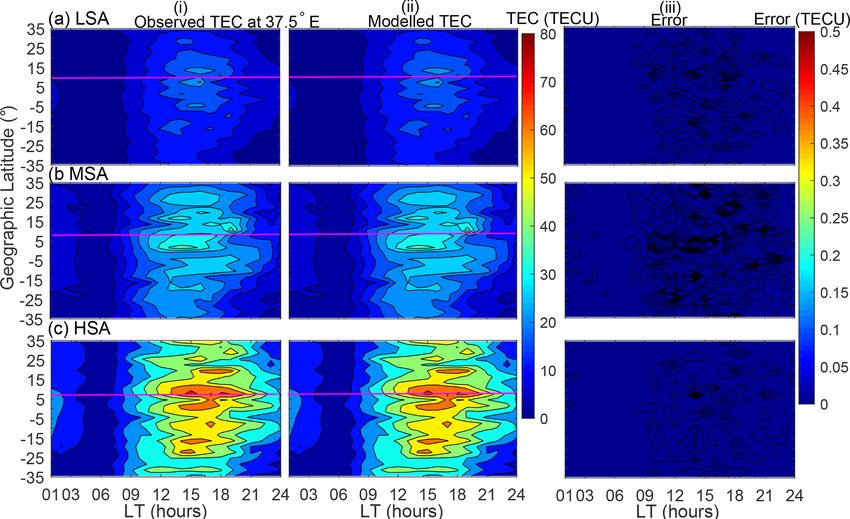
1206                                                                       P. Mungufeni et al.: Modeling total electron content

MIC data commonly consider measurements with horizontal              Table 2. Average monthly F10.7 flux values used in the study.
smear > 1500 km prone to errors, and they reject such mea-
surements. We established that after applying this restriction,                   Month              F10.7 flux (sfu)
there were ∼ 40 RO measurements per day during the year                                          LSA     MSA        HSA
2013 over our study area (not shown here). Based on the pre-
vious discussions, this value is far less than the 9216 (16 lon-                  January       71.10    83.94    140.65
gitudinal, 24 latitudinal, and 24 local time) TEC data points                     February      71.14    87.06    126.23
required in all grid cells in a day. As stated in Sect. 1, this                   March         69.81    85.40    130.98
                                                                                  April         71.02    86.09    130.46
poor amount of data to represent day-of-year TEC variation
                                                                                  May           70.29    90.59    123.80
might be the reason for the failure of the TEC model pre-                         June          69.51    89.91    118.73
sented by Okoh et al. (2019) to capture in some cases the                         July          68.09    88.14    128.92
EIA over the African region. Another reason might be the                          August        67.45    85.46    114.53
discrepancy which arises due to some locations being rep-                         September     69.20    86.34    122.98
resented by adjusted COSMIC RO TEC while others by the                            October       70.06    81.88    131.50
ground-based GPS TEC data.                                                        November      71.66    82.40    142.95
   Since empirical modeling requires adequate data for the                        December      70.82    82.97    142.72
mathematical functions to capture the physics inherent in the
data, this study did not reject COSMIC RO TEC measure-
ments with horizontal smear > 1500 km. Although not pre-             TEC were determined and used to capture the variation of
sented here, we observed that the COSMIC TEC data val-               TEC with solar flux. Table 2 presents the average F10.7 flux
ues with smear > 1500 km did not introduce alarming er-              values that were determined in the months of a year. In sum-
rors. This observation was made when we analyzed COS-                mary, a total of 331 776 TEC data values were needed to ex-
MIC TEC data which were coincident with TEC observed                 ist in 16 longitudinal, 24 latitudinal, 3 solar flux, 12 monthly,
by ionosonde stations over South Africa (see details in              and 24 hourly bins, in order to determine the model coef-
Sect. 5.2), located at Hermanus, Grahamstown, and Louis-             ficients. However, from the data of the entire study period,
vale. Interestingly, compared to measurements with hori-             only 121 447 bins were filled with TEC data values. The aver-
zontal smear > 1500 km, some measurements with horizon-              age of the standard deviations of the bins that contained more
tal smear < 1500 km were observed to be far from the lin-            than 1 TEC data during low (sample size = 21 108), medium
ear least-squares fitting line. Further analysis of COSMIC           (sample size = 6180), and high (sample size = 7495) solar
RO observations over our study area revealed that without            flux levels were 1.28, 2.15, and 4.31 TECU, respectively.
restricting horizontal smear, there were ∼ 80 RO measure-               The bins which did not have TEC data were filled by esti-
ments per day during the year 2013 (not shown here). Still           mation following the procedures described in the three steps
this value is far less than the 9216 TEC data values re-             below.
quired to fill all spatial grid cells in a day. To partially solve
this problem, instead of binning data according to year, we            1. At a particular spatial grid cell, the diurnal TEC was
binned the data according to different solar flux levels as               divided into two local time sectors, namely, (i) 10:00–
shown below.                                                              24:00 LT and (ii) 00:00–10:00 LT. Sector (i) which is
   For each spatial grid cell, the data were binned at a 1 h in-          daytime and before midnight includes the time when
terval. TEC values within the bins were averaged to yield                 daily and secondary TEC peaks are expected, while
1 h resolution TEC data over the grids. TEC data for the                  (ii) which is mostly at night is when TEC varies slowly.
different days were binned according to the F10.7 flux of                 When slow variation of TEC was expected as in sector
that day. The F10.7 flux indices were obtained from the                   (ii) and there were at least a few (> 2) TEC data avail-
Space Weather Prediction Center (SWPC) of the National                    able, a smoothing spline (De-Boor, 1978) data fitting
Oceanic and Space Administration (NOAA) (http://www.                      method was used to estimate missing TEC values. In
swpc.noaa.gov/, last access: 12 September 2020). The F10.7                cases in which rapid TEC variations are expected as in
flux ranges for low solar activity (LSA), medium solar ac-                sector (i) and at least half of the total expected number
tivity (MSA), and high solar activity (HSA) were < 76, 76–                of data points were filled with TEC data, a piece-wise
108, and > 108 sfu, respectively. The boundary values 76 and              cubic interpolation (De-Boor, 1978) data fitting method
108 sfu of the F10.7 flux ranges correspond to the 75th and               was used to estimate missing TEC values. For example,
25th percentiles of all F10.7 flux values on the days in low              when there were at least four measurements in sector
(2008–2010, 2017–2018) and high (2012–2015) solar activ-                  (ii), the missing values were obtained by evaluating the
ity years, respectively.                                                  fitted function through the existing TEC data values. On
   The data within a specific solar flux bin were further                 the other hand, when there were at least seven (half the
binned based on months of a year. The averages of the cor-                number of hours during 10:00–24:00 LT) TEC values in
responding F10.7 flux of the days used to represent seasonal              sector (i), the missing values were obtained by evaluat-

Ann. Geophys., 38, 1203–1215, 2020                                                  https://doi.org/10.5194/angeo-38-1203-2020
P. Mungufeni et al.: Modeling total electron content                                                                           1207

     ing the fitted function to the available data values. After   34.5◦ S. Figure 1 clearly shows that the available and esti-
     estimating the missing TEC data from the two sections         mated TEC variations depict the well-known diurnal and so-
     of the diurnal TEC, the entire diurnal TEC data over a        lar activity level dependence patterns. Moreover, the figure
     particular grid cell were then considered to estimate the     shows that the available data values are in most cases close
     missing values. When there were at least 12 (half the         to the estimated TEC values. Therefore, the estimated TEC
     number of hours in a day) values, the missing values          values were then used to obtain the model coefficients.
     were obtained by evaluating a smoothing spline func-
     tion fitted to the existing data values.
                                                                   3   The model
 2. At a particular latitude and local time, the values of
    TEC along all the longitudes were divided into west-           The TEC over the African region was expressed as
    ern (− 20–20◦ E) and eastern (20–60◦ E) longitude sec-
                                                                                          24 X
                                                                                             12 X
                                                                                                3 X
                                                                                                  16 X
                                                                                                     24
    tors. Each of the longitude sectors contained eight bins.                             X
                                                                   TEC(t, d, F, λ, ϕ) =                          aij klm
    At night, when there were at least three TEC values
                                                                                          i=1 j =1 k=1 l=1 m=1
    over any longitude sector, the missing values were ob-
    tained by evaluating a smoothing spline function fitted        × Ni (t) × Nj (d) × Nk (F ) × Nl (λ) × Nm (ϕ) ,               (1)
    to the available data points, while during the day, when
    there were at least four TEC values, the missing values        where the linear model coefficients aij klm were determined
    were obtained by evaluating a smoothing spline func-           by the least-squares fitting procedure to the 331 776 TEC
    tion fitted to the available data points. After estimating     data values as in Abdu et al. (2003), Jakowski et al. (2011b),
    the missing TEC values over the two longitude sectors,         and Mungufeni et al. (2015). In Eq. (1), Ni (t), Nj (d),
    the TEC over all longitudes was then considered to es-         Nk (F ), Nl (λ), and Nm (ϕ) are B splines of different orders
    timate the missing values. At night, when there were at        to represent variations of TEC with local time, seasons, solar
    least eight values, the remaining values were obtained         flux level, longitude, and latitude, respectively. Most of the
    by evaluating a smoothing spline fitted to the available       B splines were of order 2, except for those used to represent
    TEC data points. The missing values during daytime             LT and latitudinal variations which were of order 4. The or-
    were estimated when there were at least 10 measure-            der of splines used to represent LT and latitude was higher to
    ments available.                                               cater for the rapid variations of TEC with these two parame-
                                                                   ters. A total of 24 local time nodes, 1, 2, . . . , 24, were used.
 3. Procedure 3 is similar to 2, except for variations of TEC      For simple interpolation between months, seasonal/monthly
    as a function of latitude being considered at specific         nodes were placed at the 15th day of each month. Solar flux
    values of longitude and time. TEC values over the lati-        nodes used in the various months are as shown in Table 2.
    tudes were divided into lower (− 35–0◦ S) and upper (0–        The longitudinal nodes were separated by 5◦ and placed at
    35◦ N) latitudinal sectors. There were 12 bins in each of      longitudes − 17.5, 12.5 7.5, . . . , 57.5◦ , while the latitudinal
    the latitudinal sectors. To estimate missing TEC values        nodes were separated by 3◦ and placed at latitudes − 34.5,
    at night over a latitudinal sector, at least four measure-     − 31.5, − 28.5, . . . , 34.5◦ .
    ments were required to be available, while during the
    day, at least six values were required. When TEC data
    over the combined latitudinal sectors were considered          4   Comparison of observed and modeled TEC
    to estimate the missing values, at least 12 values were
    required to be available.                                      In order to assess the ability of the model to describe the data
                                                                   used to construct it, modeled data were compared with the
After repeating procedures 1–3 three times, all the 331 776        binned data that were used to solve Eq. (1). The results of the
bins were filled with TEC data. For the purposes of mini-          self-consistency check are presented in Fig. 2. It is important
mizing the effects of outliers, the diurnal TEC at spatial grid    to note that validation using data that were not included dur-
cells was then separately fitted with smoothing splines which      ing modeling is provided in Sect. 5. Panels in column (i) of
were evaluated to obtain the TEC data that were later used to      Fig. 2 present the observed binned TEC data, while column
determine the model coefficients as explained in Sect. 3. In       (ii) presents the corresponding modeled TEC data. In col-
order to demonstrate the appropriateness of our estimation of      umn (iii), we present the differences between the observed
missing TEC data values and its use for determining model          and modeled TEC data, referred to as errors. In Fig. 2, rows
coefficients, we present Fig. 1. Panels (a)–(c) of the figure      (a), (b), and (c) correspond to LSA, MSA, and HSA, respec-
present the available TEC data (∗ ) and estimated (red line)       tively. The horizontal magenta lines in Figure 2 and later also
TEC values during low, medium, and high solar flux levels,         in Fig. 3 indicate the location of ∼ 0◦ dip latitude on the cor-
respectively.                                                      responding panel. As expected, Figure 2 clearly shows that
   The TEC data plotted in Fig. 1 correspond to January            the corresponding modeled TEC almost perfectly matches
and the grid cell centered at longitude 17.5◦ W and latitude       the observed binned TEC. This can be confirmed by the small

https://doi.org/10.5194/angeo-38-1203-2020                                                 Ann. Geophys., 38, 1203–1215, 2020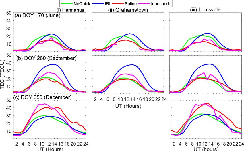
1208                                                                            P. Mungufeni et al.: Modeling total electron content

Figure 1. Panels (a–c) present available (∗ ) and estimated (red line) TEC values during low, medium and high solar flux levels, respectively.
The data are for the month of January and fall within the grid cell centered at longitude and latitude of 17.5◦ W and 34.5◦ S, respectively.

(< 0.1 TECU) error values presented in the panels of column              in the eastward electric field (Batista et al., 1986; Schunk
(iii). The variations of the ionosphere with local time and so-          and Nagy, 2009). The F layer therefore rises as the iono-
lar flux level as well as location that are exhibited in Fig. 2          sphere co-rotates into darkness. Although in the absence of
give the confidence of relying on the binned data as a good              sunlight after sunset, the lower ionosphere rapidly decays,
representation of the ionosphere. The physical explanations              there is high electron density at high altitudes, yielding the
for these variations are as follows. The increase of both ob-            secondary maximum in TEC.
served and modeled TEC that occurs when the solar flux level                Panels in rows (b) and (c) of Fig. 2 demonstrate the ex-
increases is usually attributed to increased ionizing radiations         istence of the EIA region, where there are two belts of high
in X-ray and extreme ultraviolet (EUV) bands, which in turn              electron density on both sides of 0◦ dip latitude. The EIA
leads to increased TEC in the ionosphere (Hargreaves, 1992).             is usually attributed to the upward E × B drift which lifts
   The diurnal variation of TEC matches very well with the               plasma to higher altitudes. The plasma then diffuses north
variation of photoionizing radiation. At sunrise, the electron           and south along magnetic field lines. Due to gravity and pres-
density begins to increase rapidly, owing to photoionization             sure gradient forces, there is also a downward diffusion of
(Schunk and Nagy, 2009). After this initial increase at sun-             plasma. The net effect is the formation of the EIA region
rise, electron density displays a slow rise throughout the day,          (Appleton, 1946). Another feature of EIA that can be seen in
and then it decays at sunset as the photoionization source               panels in rows (b) and (c) of Fig. 2 is the asymmetry of the
disappears. Another diurnal feature of variation of TEC ex-              crests. Along the 120◦ longitude sector, Zhang et al. (2009)
hibited in Fig. 2 is the existence of a secondary maximum                reported the asymmetry of EIA crests. As described later at
of TEC. This can clearly be seen in panels of row (c) along              the end of this section, the direction of neutral meridional
the magenta lines, where the first peak occurs at ∼ 15:00 LT             winds in March may favor high values of electron density
and the second at ∼ 18:00 LT. The formation of a secondary               over the southern crest.
maximum of TEC that was mentioned previously may be ex-                     Generally, Fig. 2 shows that the locations outside the EIA
plained as follows. During the day, the thermospheric wind               region have lower TEC values compared to locations around
generates a dynamo electric field in the lower ionosphere that           and within the EIA region. The low values of TEC over loca-
is eastward (Schunk and Nagy, 2009). The eastward elec-                  tions outside the EIA region might be due to the lower eleva-
tric field, E, in combination with the northward geomag-                 tion angle of the solar radiation flux which is responsible for
netic field, B, produces an upward E × B drift of the F re-              the creation of electrons (Schunk and Nagy, 2009). The solar
gion plasma. As the ionosphere co-rotates with the Earth to-             radiation flux is usually low for locations far from the sub-
ward dusk, the zonal (eastward) component of the neutral                 solar point. The latter situation is dominant over locations
wind increases. The increased eastward wind component, in                outside the EIA region, especially in March. The closeness
combination with the sharp day–night conductivity gradient               of the subsolar point to the locations within the EIA regions
across the terminator, leads to the pre-reversal enhancement             results in high solar radiations over these locations. As a re-

Ann. Geophys., 38, 1203–1215, 2020                                                        https://doi.org/10.5194/angeo-38-1203-2020
P. Mungufeni et al.: Modeling total electron content                                                                                 1209

Figure 2. Variation of TEC as a function of geographic latitude and local time in the March equinox at 37.5◦ E. Panels in rows (a–c) corre-
spond to LSA, MSA, and HSA, respectively, while panels in columns (i)–(iii) correspond to observed binned TEC, modeled TEC, and the
difference between observed and modeled TEC (errors), respectively. The magenta line indicates ∼ 0◦ dip latitude.

sult, high TEC values were observed over locations within               5     Model validation
the EIA region.
   To demonstrate that the modeled TEC captures TEC varia-              5.1    Validation using reserved COSMIC RO TEC
tion with season, we present Fig. 3. In the figure, columns (i)
and (ii) present observed binned TEC and the corresponding              In addition to comparing observed binned TEC with the cor-
modeled TEC, respectively. Moreover, rows (a–d) present                 responding modeled TEC, we validated our model using ob-
TEC data during March, June, September, and December, re-               served TEC in the years 2012 and 2018. The data during
spectively.                                                             these 2 years were not used in developing the model. The
   As already observed in Fig. 2, it can clearly be seen from           TEC data in the years 2012 and 2018 were binned accord-
Fig. 3 that the modeled TEC almost perfectly matches the                ing to local time and spatially in a similar manner to the data
observed TEC data. Among the many features of TEC ex-                   mentioned in Sect. 2.2. The corresponding local time, day of
hibited by both observed and modeled TEC data, we would                 year, solar flux, and spatial coordinates of the data were noted
like to emphasize the (i) equinoxial asymmetry of TEC, (ii)             and then used to generate the corresponding modeled TEC.
occurrence of lowest TEC in June solstice, and (iii) high               Despite the advantages of B spline modeling mentioned in
values of TEC in December. Features (ii) and (iii) were                 Sect. 1, one of its limitations is the inability to extrapolate.
recently reported based on similar data by Mungufeni et                 Therefore, in situations where the solar flux level is higher
al. (2019). The reader may refer to this study for more discus-         (lower) than the values specified in Table 2, the maximum
sions. Mungufeni et al. (2016) observed equinoxial asymme-              (minimum) value in the table was used to generate the cor-
try when studying ionospheric irregularities over the African           responding modeled TEC. This idea was also applied when
low-latitude region. They observed over the East African                the day of year, longitude, and latitude values were higher
region that the irregularity strength in the March equinox              (lower) than those specified in Sect. 3.
was higher than that in the September equinox. They at-                    Figure 4 presents a scatter plot showing the observed TEC
tributed the equinoxial asymmetry to meridional winds in                against the corresponding modeled TEC. The red line in the
March which might blow northward. Such a direction would                figure indicates the linear least-squares fit to the data in the
lift plasma up where recombination is not common. On the                panel. Furthermore, indicated in Fig. 4 are (i) the correlation
other hand, in September, the winds might blow southward.               coefficients (r) (ii) the r squared values, (iii) the number of
This could lead to recombination at low altitudes.                      data points (n plotted), and (iv) the root mean square error
                                                                        (RMSE) when the modeled TEC is used to represent the ob-
                                                                        served TEC.

https://doi.org/10.5194/angeo-38-1203-2020                                                       Ann. Geophys., 38, 1203–1215, 2020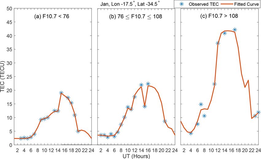
1210 P. Mungufeni et al.: Modeling total electron content
Figure 3. Variation of TEC as a function of latitude and local time in HSA at 37.5◦ E. Panels in rows (a–d) are for the March equinox,
June solstice, September equinox, and December solstice, respectively, while panels in columns (i) and (ii) are observed binned and modeled
TEC, respectively. The magenta line indicates 0◦ dip latitude.
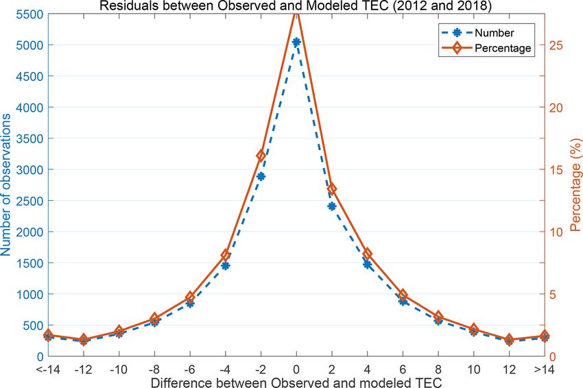
Figure 4. Scatter plot of observed TEC against modeled TEC. Figure 5. The blue and red curves show the distribution of the num-
ber of observed errors (difference between observed and modeled
TEC) and the percentage of the errors, respectively.
The following observations can be noted from Fig. 4.
(i) The modeled TEC correlates highly (r ∼ 0.93) with the referred to as errors. We also computed the percentage of
observed TEC. (ii) The r squared values indicate that high the different errors. The left and right vertical axes in Fig. 5
proportions (∼87 %) of the variations in the observed TEC present the distribution of the number of observed errors and
can be predicted by the modeled TEC. (iii) The RMSE value their percentages, respectively. It can be seen from the figure
of 5.05 TECU signifies that the modeled TEC closely ap- that the errors are randomly distributed since the distribution
proximates the observed TEC. curve is symmetric about 0 TECU. Indeed, the magnitudes
In order to show that the observed and modeled TEC have of the modeled TEC values are close to those of the observed
similar magnitudes in addition to their similar variation de- TEC since the majority of the error values are close to zero.
picted in Fig. 4, we computed the differences between corre- The cases of high error values (> 10 TECU) mostly have
sponding values of the data plotted in the figure. These were < 2.5 % occurrence probability, as can be seen on the right
Ann. Geophys., 38, 1203–1215, 2020 https://doi.org/10.5194/angeo-38-1203-2020P. Mungufeni et al.: Modeling total electron content 1211
vertical axis. These high errors may be partly attributed to Table 3. Correlation coefficients, r and RMSE associated with esti-
the limitation of the spline modeling technique (inability to mation of TEC observed by ionosonde stations using models.
extrapolate) which was discussed earlier in this subsection,
Sect. 5.1. Ionosonde station/ Model r RMSE
number of observations (TECU)
5.2 Validation using ionosonde TEC measurements Hermanus Spline 0.92 4.64
(n = 5110) IRI-2016 0.86 5.45
The TEC data measured by the digisonde ionosonde stations NeQuick 2 0.92 4.10
over South Africa located at Hermanus, Grahamstown, and
Grahamstown Spline 0.88 5.56
Louisvale can be accessed from the National Oceanic and At- (n = 4450) IRI-2016 0.82 6.29
mospheric Administration (NOAA) website via the link ftp: NeQuick 2 0.86 5.27
//ftp.ngdc.noaa.gov (last access: 12 September 2020). The
data obtained from the NOAA website are in the form of Louisville Spline 0.94 3.82
auto-scaled ionospheric parameters such as peak height in the (n = 4543) IRI-2016 0.87 5.62
NeQuick 2 0.94 3.73
F2 layer, critical frequency in the F2 layer, and TEC which
are stored in Standard Archiving Output (SAO) format files.
It should be noted that the TEC data provided in SAO files
are obtained by integrating electron density profiles up to al- TEC was estimated using the models listed in column 2. The
titudes of ∼ 700 km. More details about the auto-scaling pro- number of observations (n) over each station that were used
gram (real-time ionogram scaler with true height (ARTIST)) to determine r and RMSE are put in brackets below the sta-
and the electron density profiles they produce can be found tion name.
in Reinisch and Huang (2001) and Klipp et al. (2020). It can be seen from Table 3 that the r values associated
The magenta lines in Fig. 6 present the diurnal patterns of with NeQuick 2 and the spline-based model are consistently
TEC measured by ionosonde stations at Hermanus (panels in better when compared with those of IRI-2016. Moreover, the
column i), Grahamstown (panels in column ii), and Louisvale RMSE values associated with IRI-2016 are the highest in all
(panels in column iii). The corresponding TEC generated by the cases. These two observations indicate that compared to
our spline modeling technique (spline), NeQuick 2, and IRI- the spline model and NeQuick 2, IRI-2016 poorly estimates
2016 is superimposed with red, green, and blue lines, respec- TEC at the locations of the ionosondes. The RMSE values as-
tively. We need to mention that during computation of TEC sociated with NeQuick 2 are always slightly lower than that
using NeQuick 2 and IRI-2016, the height was limited to of the spline model, while the r values associated with the
the approximate altitude of the COSMIC satellites (800 km). spline model are mostly comparable or slightly higher than
Moreover, for the case of IRI-2016, the NeQuick model op- that of NeQuick 2. These discussions demonstrate that our
tion was specified to estimate topside electron density. spline model generates TEC values consistently with that ob-
The panels in rows (a)–(c) show TEC on day of year 170 served by ionosondes. This implies that equivalent TEC mea-
(June), 260 (September), and 350 (December), respectively. sured by ionosondes over midlatitude locations which do not
These three days of the year in 2013 were geomagnetically have ionosonde stations can be predicted fairly well using our
quiet. Preliminarily, Fig. 6 appears to reveal that IRI-2016 ei- model. We might validate our model over the low-latitude
ther overestimates (December) or underestimates (June and region that falls within the current study area if ionosonde
September) the TEC measured by the ionosonde stations. On observations become available over the region in future.
the other hand, our spline modeling technique and NeQuick
2 seem to depict good correspondence between the observed 5.3 Comparison of our model with existing regional
and the modeled TEC. It can also be seen from Fig. 6 that models
over a particular station, the shape of curves on different days
representing TEC generated by the IRI-2016 and NeQuick 2 It would be good to compare error levels produced when
models is similar. This is expected since these two models some measured TEC values are compared with modeled
were meant to reproduce monthly median values of the iono- TEC generated by (i) the existing regional TEC models
sphere. This means that our model, based on spline functions, discussed in Sect. 1 and (ii) our TEC model of the spline
may capture the day-to-day variability of the ionosphere bet- technique. We may not perform such analysis since models
ter. in (i) are based on electron density integrated from the
We generated such data plotted in Fig. 6 for geomagneti- ground up to GPS satellites (∼ 20 200 km), while the model
cally quiet days of the entire year 2013 and then performed in (ii) is based on electron density integrated up to ∼ 800 km.
statistical analysis of the observed and the model TEC data. However, we present Figs. 7 and 8 to compare EIA features
Table 3 presents in column 3 the correlation coefficients (r) captured by our spline modeling technique with those by
for the correlations between modeled and ionosonde TEC. the neural network technique of Okoh et al. (2019). The
Moreover, the table presents the RMSE when the ionosonde TEC plots based on the neural network technique can be
https://doi.org/10.5194/angeo-38-1203-2020 Ann. Geophys., 38, 1203–1215, 20201212 P. Mungufeni et al.: Modeling total electron content
Figure 6. Magenta color shows diurnal TEC observed by ionosonde stations at Hermanus (panels in column i), Grahamstown (Panels in
column ii), and Louisvale (Panels in column iii). The green, blue, and red colors show TEC estimations using NeQuick 2, IRI-2016, and
spline models, respectively. Panels in rows (a–c) show diurnal TEC during the year 2013 on DOY 170, 260, and 350, respectively.
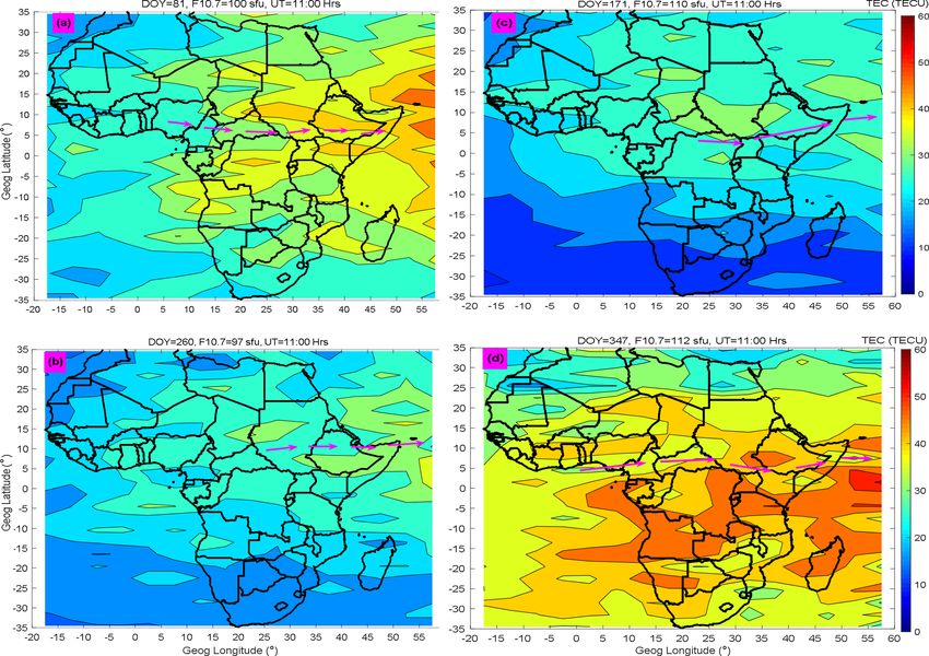
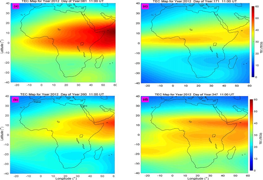
obtained from the MATLAB central website (Okoh et nique produces results (see Fig. 2) which demonstrate that
al., 2019). (https://www.mathworks.com/matlabcentral/ the modeled data match the observed data almost perfectly,
fileexchange/69257-african-gnss-tec-afritec-model?s_tid= it is expected that the spatial variations of TEC in maps of
prof_contriblnk, last access: 12 September 2020). We Fig. 8 are not smooth.
present in Fig. 7 examples of TEC generated by the neural
network model during the year 2012 at 11:00 UT. Over the
East African sector (LT = UT + 3), this time translates to
14:00 LT and falls within the range of LT when EIA exists 6 Conclusions
over the region (Mungufeni et al., 2018). Panels (a) and
(b) in Fig. 7 present TEC during March (DOY 81) and This study developed a model of TEC measured by COS-
September (DOY 260) equinoxes, respectively, while (c) MIC satellites. The TEC data were binned according to lo-
and (d) present TEC during June (DOY 171) and December cal time, seasons, solar flux level, and spatially. The coeffi-
(DOY 347) solstices, respectively. It is important to mention cients of B splines that were fitted to the binned data were
that these four days were geomagnetically quiet. determined by means of the least-squares procedure. As ex-
In order to generate TEC maps using our model for pur- pected, the modeled TEC almost perfectly matched the cor-
poses of comparing with TEC maps in Fig. 7, we noted and responding observed binned TEC data. The model was vali-
used the F10.7 flux values on the days indicated in the figure. dated with independent data that were not used in the model
The TEC maps generated using our model that correspond to development. The validation revealed that (i) the observed
TEC maps presented in Fig. 7 are presented in Fig. 8. and the modeled TEC correlate highly (r = 0.93), (ii) the
Unlike our TEC maps in Fig. 8 which clearly show the EIA coefficient of determination R 2 which is the proportion of
trough (see magenta arrows) in all the seasons, the neural net- variance in the observed data predicted by our model was
work technique TEC maps (Okoh et al., 2019) of Fig. 7 only 87 %, and (iii) the modeled TEC closely approximates the
clearly capture the EIA trough in the December solstice. As observed TEC (RMSE of 5.05 TECU). Due to the exten-
pointed out before, this shortfall in the neural network TEC sive input data and the modeling technique applied, we were
model might be due to a poor amount of data to represent able to reproduce the well-known features of TEC variation
the day of year during model development. Another obser- over the African region. Further validation of our model us-
vation that can be made from Figs. 7 and 8 is that unlike the ing TEC obtained from ionosonde stations over South Africa
neural network model which yields smooth spatial TEC vari- at Hermanus, Grahamstown, and Louisville reported r val-
ation, the spline modeling technique does not yield smooth ues > 0.92 and RMSE < 5.56 TECU. These validation re-
spatial TEC variation. In real life, measurement or observed sults imply that our model can estimate TEC fairly well that
values rarely vary smoothly. Since the spline modeling tech- would be measured by ionosondes over locations which do
not have the instrument.
Ann. Geophys., 38, 1203–1215, 2020 https://doi.org/10.5194/angeo-38-1203-2020P. Mungufeni et al.: Modeling total electron content 1213 Figure 7. Neural network TEC maps during the year 2012 at 11:00 UT. Panels (a) and (b) are for March (DOY 81) and September (DOY 260) equinoxes, respectively, while (c) and (d) are for June (DOY 171) and December (DOY 347) solstices, respectively. Figure 8. Similar to Fig. 7 but generated by the spline modeling technique. Magenta arrows indicate approximate locations of the EIA trough. https://doi.org/10.5194/angeo-38-1203-2020 Ann. Geophys., 38, 1203–1215, 2020
1214                                                                           P. Mungufeni et al.: Modeling total electron content

Data availability. Dst data are provided by the World Data Center           F region to different geomagneticstorms observed by GPS
for Geomagnetism at Kyoto (http://swdcwww.kugi.kyoto-u.ac.jp/,              in the African sector, J. Geophys. Res., 116, A12319,
last access: 12 September 2020; Nose et al., 2020). Kp data are pro-        https://doi.org/10.1029/2011JA016998, 2011.
vided by GFZ Potsdam at ftp://ftp.gfz-potsdam.de/pub/home/obs/           Appleton, E. V.: Two Anomalies in the Ionosphere, Nature, 3995,
kp-ap/ (last access: 12 September 2020; Matzka and Stolle, 2020).           p. 691, 1946.
F10.7 flux data were obtained from http://www.swpc.noaa.gov/             Batista, I. S., Abdu, M. A., and Bittencourt, J. A.: Equatorial F re-
(last access: 12 September 2020; U.S. Dept. of Commerce, 2020)              gion vertical plasma drifts: seasonal and longitudinal asymme-
while ionPrf files used to derive COSMIC TEC were obtained                  tries in the American sector, J. Geophys. Res., 91, 12055–12064,
from http://cosmic-io.cosmic.ucar.edu/cdaac/index.html (last ac-            1986.
cess: 12 September 2020; COSMIC Data Analysis Center, 2020).             Bilitza, D.: International Reference Ionosphere 2000, Radio Sci.,
We thank NOAA for making ionosonde data available via the link              36, 757–767, 2001.
ftp://ftp.ngdc.noaa.gov (last access: 12 September 2020; Gamache         Bolaji, O., Owolabi, O., Falayi, E., Jimoh, E., Kotoye, A.,
et al., 2020).                                                              Odeyemi, O., Rabiu, B., Doherty, P., Yizengaw, E., Yamazaki,
                                                                            Y., Adeniyi, J., Kaka, R., and Onanuga, K.: Observations of
                                                                            equatorial ionization anomaly over Africa and Middle East dur-
Author contributions. PM wrote the first draft of the manuscript            ing a year of deep minimum, Ann. Geophys., 35, 123–132,
and wrote the MATLAB codes to analyze the data. He incorporated             https://doi.org/10.5194/angeo-35-123-2017, 2017.
suggestions made by co-authors and reviewers to the manuscript           Buonsanto, M. J.: Ionospheric Storms – A Review, Space Sci. Rev.,
in order to realize the current version of the article. SS evaluated        88, 563–601, 1999.
the objectives of the first draft of the manuscript and suggested        COSMIC data analsysis center: Level 2 – ionospheric profiles,
some of the validation data of the model developed in this arti-            available at: http://cosmic-io.cosmic.ucar.edu/cdaac/index.html,
cle. YMO provided guidance about Fortran codes for generating               last access: 12 September 2020.
TEC from NeQuick and IRI models. She also intensely evaluated            De-Boor, C.: A Practical Guide to Splines, Springer, New York,
the manuscript and made suggestions before it was submitted for             USA, 1978.
reviewing. YHK suggested comparison of the model developed in            Emmert, J. T., Richmond, A. D., and Drob, D. P.: A computa-
this article with the existing models. Moreover, he intensely evalu-        tionally compact representation of Magnetic-Apex and Quasi-
ated the manuscript and made suggestions which were incorporated            Dipole coordinates with smooth base vectors, J. Geophys. Res.,
before it was submitted for reviewing.                                      15, A08322, https://doi.org/10.1029/2010JA015326, 2010.
                                                                         Ercha, A., Zhang, D., Ridley, A. J., Xiao, Z., and Hao, Y.: A global
                                                                            model: Empirical orthogonal function analysis of total elec-
Competing interests. The authors declare that they have no conflict         tron content 1999–2009 data, J. Geophys. Res., 117, A03328,
of interest.                                                                https://doi.org/10.1029/2011JA017238, 2012.
                                                                         Gamache, R. R., Galkin, I. A., and Reinisch, B. W.: A Database
                                                                            Record Structure for Ionogram Data, University of Lowell Center
                                                                            for Atmospheric Research, available at: ftp://ftp.ngdc.noaa.gov,
Acknowledgements. The first author greatly appreciates the im-
                                                                            last access: 12 September 2020.
mense contribution of Claudia Stolle towards shaping the presenta-
                                                                         Guochang, X.: GPS. Theory, Algorithms, and Applications,
tion of the paper. We thank the developers of the IRI and NeQuick
                                                                            Springer, New York, USA, 2007.
models for making their models available.
                                                                         Habarulema, J. B., McKinnel, L., and Opperman, B.: Regional GPS
                                                                            TEC modeling; attempted spatial and temporal extrapolation of
                                                                            TEC using neural networks, J. Geophys. Res.-Space Phys., 116,
Financial support. The research has been supported by the fund              A04314, https://doi.org/10.1029/2010JA016269, 2011.
from the Air Force Research Laboratory of the United States of           Hargreaves, J. K.: The Solar-Terrestrial environment, Cambridge
America (grant no. FA2386-19-1-0123) to Chungnam National                   University Press, New York, USA, 1992.
University.                                                              Hofmann-Wellenhof, B., Lichtenegger, H., and Wasle, E.: Global
                                                                            Navigation Satellite Systems, GPS, GLONASS, Galileo and
                                                                            more, Springer, New York, USA, 2007.
Review statement. This paper was edited by Dalia Buresova and            Jakowski, N., Hoque, M. M., and Mayer, C.: A new global TEC
reviewed by Rolland Fleury and two anonymous referees.                      model for estimating trans-ionospheric radio wave propagation
                                                                            errors, J. Geod., 85, 965–974, 2011a.
                                                                         Jakowski, N., Schlüter, S., and Sardon, E.: Total electron content
                                                                            models and their use in ionosphere monitoring, Radio Sci., 46,
References                                                                  RS0D18, https://doi.org/10.1029/2010RS004620, 2011b.
                                                                         Klipp, T. D. S., Petry, A., de Souza, J. R., de Paula, E. R., Fal-
Abdu, M. A., Souza, J. R., Batista, I. S., and Sobral, J. H. A.: Equa-      cão, G. S., and de Campos Velho, H. F.: Ionosonde total elec-
  torial spread F statistics and empirical representation for IRI:          tron content evaluation using International Global Navigation
  A regionalmodel for the Brazilian longitude sector, Adv. Space            Satellite System Service data, Ann. Geophys., 38, 347–357,
  Res., 31, 703–716, 2003.                                                  https://doi.org/10.5194/angeo-38-347-2020, 2020.
Adewale, A. O., Oyeyemi, E. O., Adeloye, A. B., Ng-
  wira, C. M., and Athieno, R.: Responses of equatorial

Ann. Geophys., 38, 1203–1215, 2020                                                       https://doi.org/10.5194/angeo-38-1203-2020
P. Mungufeni et al.: Modeling total electron content 1215 Klobuchar, J. A.: Ionospheric time-delay algorithm for single fre- Okoh, D., Owolabi, O., Ekechukwu, C., Folarin, O., Arhiwo, G., quency GPS users, IEEE Trans. Aerosp. Electron. Syst., 23, 325– Agbo, J., Bolaji, S., and Babatunde, R.: A regional GNSS-VTEC 331, https://doi.org/10.1109/TAES.1987.3-10829, 1987. model over Nigeria using neural networks: A novel approach, Krankowski, A., Zakharenkova, I., Krypiak-Gregorczyk, A., Shag- Geodesy and Geodynamics, 7, 19–31, 2016. imuratov, I. I., and Wielgosz, P: Ionospheric electron density Okoh, D., Seemala, G., Rabiu, B., Habarulema, J. B., Jin, S., observed by FORMOSAT-3/COSMIC over the European re- Shiokawa, K., Otsuka, Y., Aggarwal, M., Uwamahoro, J., gion and validated by ionosonde data, J. Geodesy, 85, 949–964, Mungufeni, P., Segun, B., Obafaye, A., Ellahony, N., Okonkwo, https://doi.org/10.1007/s00190-011-0481-z, 2011. C., Tshisaphungo, M., and Shetti, D.: A Neural Network-Based Leva, J. L., de Haag, M. U., and Dyke, K. V.: Performance of stan- Ionospheric Model Over Africa From Constellation Observing dalone GPS, in: Understanding GPS: Principles and Applica- System for Meteorology, Ionosphere, and Climate and Ground tions, edited by: Kaplan, E. D. and Hegarty, C. J., Artech House, Global Positioning System Observations, J. Geophys. Res.- Inc. 685 Canton Street Norwood, MA 02062, 66–112, 2006. Space, 124, https://doi.org/10.1029/2019JA027065, 2019. Nose, M., Iyemori, T., Sugiura, M., and Kamei, T.: Geomag- Opperman, B.: Reconstructing ionospheric TEC over South Africa netic Dst index, World Data Center for Geomagnetism, Kyoto, using signals from a regional GPS network, PhD Thesis, Rhodes available at: http://swdcwww.kugi.kyoto-u.ac.jp/, last access: 12 University, Grahamstown, South Africa, 30 pp., 2008. September 2020. Rama Rao, P. V. S., Jayachandran, P. T., Sri Ram, P., Ramana Rao, Matzka, J. and Stolle, C.: Indices of Global Geomagnetic Ac- B. V., Prasad, D. S. V. V. D., and Bose, K. K.: Characteristics of tivity, World Data Center for Geomagnetism, Kyoto, available VHF radiowave scintillations over a solar cycle (1983–1993) at a at: ftp://ftp.gfz-potsdam.de/pub/home/obs/kp-ap/, last access: 12 low-latitude station: Waltair (17.7◦ N, 83.3◦ E), Ann. Geophys., September 2020. 15, 729–733, https://doi.org/10.1007/s00585-997-0729-3, 1997. Mengist, C. K., Ssessanga, N., Jeong, S.-H., Kim, J.-H., Reinisch, B. and Huang, X.: Deducing topside profiles and total Kim, Y. H., and Kwak, Y.-S: Assimilation of multiple electron content from bottomside ionograms, Adv. Space Res., data types to a regional ionosphere model with a 3D- 27, 23–30, https://doi.org/10.1016/S0273-1177(00)001368, Var algorithm (IDA4D), Space Weather, 17, 1018–1039, 2001. https://doi.org/10.1029/2019SW002159, 2019. Rishbeth, H. and Garriot, O. K.: Introduction to Ionospheric Mukhtarov, P., Pancheva, D., Andonov, B., and Pashova, L.: Global Physics, Academic Press, New York, USA, 1969. TEC maps based on GNSS data: 1. Empirical background TEC Scherliess, L. and Fejer, B. G.: Radar and satellite global equatorial model, J. Geophys. Res.-Space, 118, 4594–4608, 2013. F-region vertical drift model, J. Geophys. Res., 104, 6829–6842, Mungufeni, P., Jurua, E., Habarulema, J. B., and Anguma, S. K.: 1999. Modeling the probability of ionospheric irregularity occurrence Schunk, W. R. and Nagy, F. A.: Ionospheres: Physics, Plasma over African low latitude region, J. Atmos. Sol.-Terr. Phy., 128, Physics, and Chemistry, Cambridge University press, New York, 46–57, 2015. USA, 2009. Mungufeni, P., Habarulema, J. B., and Jurua, E. A.: Trends of Sun, Y., Liu, J., Tsai, H., and Krankwski, A.: Global ionospheric ionospheric irregularities over African low latitude region dur- map constructed by using TEC from ground-based GNSS re- ing quiet geomagnetic conditions, J. Atmos. Sol.-Terr. Phy., 14, ceiver and FORMSAT-3/COSMIC GPS occultation experiment, 261–267, 2016. GPS solutions, 21, 1583–1591, https://doi.org/10.1007/s10291- Mungufeni, P., Habarulema, J. B., Migoya-Orué, Y., and Jurua, 017-0635-4, 2017. E.: Statistical analysis of the correlation between the equato- Tebabal, A., Radicella, S. M., Damtie, B., Migoya- rial electrojet and the occurrence of the equatorial ionisation Orue’, Y., Nigussie, M., and Nava, B.: Feed forward anomaly over the East African sector, Ann. Geophys., 36, 841– neural network based ionosphericmodel for the East 853, https://doi.org/10.5194/angeo-36-841-2018, 2018. African region, J. Atmos. Sol.-Terr. Phy., 191, 1–10, Mungufeni, P., Rabiu, A. B., Okoh, D., and Jurua, E.: Characteriza- https://doi.org/10.1016/j.jastp.2019.05.016, 2019. tion of Total Electron Content over African region using Radio Thébault, E., Finlay, C. C., Beggan, C. D., Alken, P., Aubert, Occultation observations of COSMIC satellites, Adv. Space Res., J., Barrois, O., Bertrand, F., Bondar, T., and Bones, A.: In- 65, 19–29, https://doi.org/10.1016/j.asr.2019.08.009, 2019. ternational Geomagnetic Reference Field: the 12th generation, Najman, P. and Kos, T.: Performance Analysis of Empirical Iono- Earth Planet. Sp., 79, 67–79, https://doi.org/10.1186/s40623- sphere Models by Comparison with CODE Vertical TEC Maps, 015-0228-9, 2015. in: Mitigation of Ionospheric Threats to GNSS: an Appraisal U.S. Dept. of Commerce, NOAA: Daily Solar Data, Space Envi- of the Scientific and Technological Outputs of the TRANSMIT ronment Center, available at: http://www.swpc.noaa.gov/, last ac- Project, edited by: Notarpietro, R., InTech Open Science Publica- cess: 12 September 2020. tions, 5 Princes Gate Court, London, SW7 2QJ, United Kingdom, Zhang, M.-L., Wan, W., Liu, L., and Ning, B.: Variability study 162–178, https://doi.org/10.5772/58774, 2014. of the crest-to-trough TEC ratio of the equatorial ionization Nava, B., Coïsson, P., and Radicella, S. M.: A new version of the anomaly around 120◦ E longitude, Adv. Space Res., 43, 1762– NeQuick ionosphere electron density model, J. Atmos. Sol.-Terr. 1769, 2009. Phy., 70, 1856–1862, 2008. https://doi.org/10.5194/angeo-38-1203-2020 Ann. Geophys., 38, 1203–1215, 2020
You can also read