Impact Assessment for Building Energy Models Using Observed vs. Third-Party Weather Data Sets - MDPI
←
→
Page content transcription
If your browser does not render page correctly, please read the page content below
sustainability

Article
Impact Assessment for Building Energy Models
Using Observed vs. Third-Party Weather Data Sets
Eva Lucas Segarra 1, *,† , Germán Ramos Ruiz 1,† , Vicente Gutiérrez González 1 ,
Antonis Peppas 2 , Carlos Fernández Bandera 1
 1   School of Architecture, University of Navarra, 31009 Pamplona, Spain; gramrui@unav.es (G.R.R.);
     vgutierrez@unav.es (V.G.G.); cfbandera@unav.es (C.F.B.)
 2   School of Mining and Metallurgical Engineering, National Technical University of Athens (NTUA),
     15780 Athens, Greece; peppas@metal.ntua.gr
 *   Correspondence: elucas@unav.es; Tel.: +34-948-425-600 (ext. 800000)
 †   These authors contributed equally to this work.

 Received: 20 July 2020; Accepted: 17 August 2020; Published: 21 August 2020

 Abstract: The use of building energy models (BEMs) is becoming increasingly widespread for
 assessing the suitability of energy strategies in building environments. The accuracy of the results
 depends not only on the fit of the energy model used, but also on the required external files, and the
 weather file is one of the most important. One of the sources for obtaining meteorological data for a
 certain period of time is through an on-site weather station; however, this is not always available
 due to the high costs and maintenance. This paper shows a methodology to analyze the impact on
 the simulation results when using an on-site weather station and the weather data calculated by a
 third-party provider with the purpose of studying if the data provided by the third-party can be
 used instead of the measured weather data. The methodology consists of three comparison analyses:
 weather data, energy demand, and indoor temperature. It is applied to four actual test sites located
 in three different locations. The energy study is analyzed at six different temporal resolutions in
 order to quantify how the variation in the energy demand increases as the time resolution decreases.
 The results showed differences up to 38% between annual and hourly time resolutions. Thanks to
 a sensitivity analysis, the influence of each weather parameter on the energy demand is studied,
 and which sensors are worth installing in an on-site weather station are determined. In these test
 sites, the wind speed and outdoor temperature were the most influential weather parameters.

 Keywords: weather file management; weather datasets; weather stations; building energy simulation;
 sensitivity analysis of weather parameters; thermal zone temperature

1. Introduction
     The sustainable development goals report of 2019 highlighted the concern of the United Nations
toward a more sustainable world where people can live peacefully on a healthy planet. One of the
most important areas for the protection of our planet is the actions to mitigate climate change. “If we
do not cut record-high greenhouse gas emissions now, global warming is projected to reach 1.5 ◦ C in the
coming decades” [1]. This concern was also endorsed by 186 parties in the Paris agreement on climate
change in 2015 [2]. One of the strategies for tackling climate change is to reduce energy consumption
(by increasing the system efficiency) and increase the use of clean energy so that greenhouse gas
emissions are reduced. In this process of decarbonization, the buildings and the construction sector
are critical elements, since as the Global Status Report for Buildings and Construction highlighted,
they are responsible “for 36% of final energy use and 39% of energy and process-related carbon dioxide (CO2 )

Sustainability 2020, 12, 6788; doi:10.3390/su12176788                     www.mdpi.com/journal/sustainability
Sustainability 2020, 12, 6788 2 of 27
emissions in 2018, 11% of which resulted from manufacturing building materials and products such as steel,
cement and glass.” [3].
For this reason, building energy models (BEMs) play an important role in the understanding
of how to reduce the energy consumed by buildings (lighting, equipment, heating, ventilation, and
air-conditioning (HVAC) systems, etc.) and how to optimize their use. As Nguyen et al. highlighted,
there is a huge variety of building performance simulation tools [4], and EnergyPlus is one of the most
used [5]. In any simulation program, to obtain reliable results, the model must not only be adjusted
to the behavior of the building, but all the files on which it depends must be reliable and suitable for
the use that will be given to the model. Of all these files, the weather file is, perhaps, one of the most
important [6].
Bhandari et al. highlighted that there are three kinds of weather data files, typical, actual, and future,
which should be selected according to the use of the energy model [6]. The first corresponds to a
representation of the weather pattern of a specific place taking into account a set of years (commonly
20–30 years). For each month, the data are selected from the year that was considered most “typical” for
that month so that it represents the most moderate weather conditions, excludes weather extremities,
and reflects long-term average conditions for a location. In general, they are used to design and study
the behavior of the building under standard conditions, to obtain Energy Performance Certificates,
to study the feasibility of a building’s refurbishment, etc. The typical files are not recommended in
extreme conditions, such as designing HVAC systems for the worst case scenario.
There are two main sources of typical weather files: those developed by the National Renewable
Energy Laboratory (NREL), which come from stations in the United States and its territories, where the
different versions (typical meteorological year (TMY), TMY2, and TMY3) take into account different
numbers of stations, time periods, solar radiation considerations, etc. [7,8]; and those developed by the
American Society of Heating, Refrigerating and Air-Conditioning Engineers (ASHRAE) as a result of
the ASHRAE Research Project 1015 [9,10]: the International Weather for Energy Calculations (IWEC),
which takes into account weather stations outside the United States and Canada. The latest version
(IWEC2) covers 3012 worldwide locations [11] taking into account a 25 year period (1984–2008) from
the Integrated Surface Hourly (ISH) weather database.
The second kind of weather data file, actual, corresponds to a specific location and time period.
It could be obtained from an on-site weather station or by processing data from several nearby stations.
The latter option is commonly used by external data providers. This type of file is usually used to
carry out building energy model calibrations, calculate energy bills and utility costs, study the specific
behavior of HVAC systems, etc. As can be seen, these files take into account extraordinary situations,
such as heat waves, adverse or extraordinary atmospheric phenomena, etc. [12].
Finally, the last kind of weather data file, future, is mainly used to simulate how it is possible to
adapt the building energy demand to an external energy requirement (demand response [13]) or to
obtain better use strategies of HVAC systems in certain situations (model predictive control [14,15]).
As Lazos et al. highlighted, there are three common groups of forecasting techniques: statistical,
machine learning, and physical and numerical methods [16].
Therefore, each kind of weather data file has a certain purpose; therefore, the reliability of the
results will largely depend on the accuracy and suitability of the file selected [17,18].
Many studies highlighted the importance of the weather file when performing building energy
analysis, as its accuracy is generally assumed, although it is out of the control of the person in charge
of the simulation, its difference being significant. The following are some examples of studies that use
typical weather files for different applications where the weather data are relevant. It is meaningful
in retrofitting scenarios [19], or when quantifying renewable energy as in the cases when sizing
photovoltaic solar panels [20], or when used to obtain ground temperatures [21], even when studying
climate change; the accuracy of the weather files is also very important, as they are the baseline files in
the process of morphing the data [22–24]. Therefore, when using such files, it is important to try to use
the most recent [25].Sustainability 2020, 12, 6788 3 of 27
There are other studies that analyze the building energy performance using actual weather
files, either from commercial vendors [26], or developed using nearby weather stations, not located
in the building [6,27–29], or the lesser ones, from weather stations placed in the building or in
its surroundings [30]. Finally, regarding the future weather files, the uncertainty of the forecast
files is closely related to the accuracy of the files on which they are based [31–33]. There are many
studies that highlight the importance of the weather files, measuring, for example, their impact on
passive buildings [34], on micro-grids [35,36], etc., calculating the loads of district energy systems [37],
the electricity consumption with demand response strategies [13], or evaluating the effect on comfort
conditions [38]. Some analyzed the effect that certain parameters of the weather file have, emphasizing
the temperature as the most sensitive value for load forecasting [39,40].
In terms of temporal resolutions, most research focused on annual results when comparing
different sets of weather data. Wang et al. analyzed the uncertainties in annual energy consumption
due to weather variations and operation parameters for a reference office prototype, concluding that
uncertainties caused by operation parameters were much more significant than weather variations [26].
Crawley et al. analyzed the energy results using measured weather data for 30 years and several
weather datasets for a set of five locations in the USA, and the variation in annual energy consumption
was on average ±5% [17]. Seo et al. conducted a similar study, also analyzing the peak electrical
demand with similar results: a maximum difference of 5% [41].
In terms of research that focused on monthly criteria, Bhandari et al. found that, when using
different weather datasets, the annual energy consumption could vary around ±7%, but up to ±40%
when monthly analysis was performed [6]. Radhi compared the building’s energy performance of
using past and recent (up-to-date) weather data with annual and monthly criteria. This showed a
difference of 14.5% between the annual electricity consumption simulated with past data and actual
consumption, while this difference grew up to 21% for one month when monthly criteria were used [42].
Finally, there were a few studies where the temporal resolution was less than one month. With weekly
criteria, Silvero et al. compared five different weather data sources with the observed meteorological
data, showing that, for the annual criteria, the results were similar, but for the hottest and coldest
weeks of the year, the inaccuracies increased [28].
The aim of this work is to show how to evaluate the impact of using two different actual weather
datasets on the building energy model simulations, measuring both their effect on energy demand
and indoor temperature. The purpose is to analyze if the data provided by the on-site weather stations
(with a high economic cost and maintenance) could be replaced by the actual data provided by a
third-party. For this study, four test sites based on real buildings were used to compare the existing
variations when weather files with data obtained from real stations and external provider were used
in the simulations. These test sites are part of an EU funded H2020 research and innovation project
SABINA (SmArt BI-directional multi eNergy gAteway) [43], which aims to develop new technology
and financial models to connect, control, and actively manage the generation and storage of assets to
exploit synergies between electrical flexibility and the thermal inertia of buildings. The energy demand
variation analysis was measured by grouping it into different periods (annual, seasonal, monthly,
weekly, daily, and hourly) since as explained by ASHRAE [44], “. . . the aggregated data will have a reduced
scatter and associated CV(RMSE), favoring a model with less granular data.” The objective of the paper is to
highlight these differences in the results when using different granular criteria since, depending on
the use of the building energy model, their influence can be significant, for example for calibration
purposes, where the monthly or hourly criteria are required. A sensitivity analysis was also performed
to evaluate the influence of each weather parameter on the energy demand variation when using the
two different actual weather datasets.
The main contributions of this research are: (1) four real test sites, with different uses and
architectural characteristics, located in three different climates were employed in the study; (2) while
most of studies that analyze weather data influence in building energy simulation use the typical
meteorological year (TMY) [19–24], this study performed a comparison of two actual datasets: on-siteSustainability 2020, 12, 6788 4 of 27
and third-party weather data; (3) when the studies used actual weather data, they usually lacked a
local weather station due to its expensive installation [6,27–29]; instead, the observed weather data
from this study were provided by three weather stations installed on the building roofs or in their
surroundings, providing on-site measurements; and (4) the energy results are shown with different
temporal resolutions (from annual to hourly) in order to highlight the differences in the variations
when the data are accumulated.
The paper is structured as follows. In Section 2, we describe the methodology used to analyze
both the differences between the on-site and third-party weather datasets and the variation produced
by these weather files in the results of the simulations in terms of the energy demand and in terms
of the indoor temperature. In Section 3, we show the results obtained from the different approaches:
the weather datasets comparison (Section 3.1), energy demand (Section 3.2), and indoor temperature
(Section 3.3). Finally, in Section 4, we discuss the results obtained in the study, and in Section 5,
the conclusions are presented.
2. Methodology
Figure 1 shows the diagram of the methodology used in this study and the three analyses that
were performed: (1) the weather data comparison between the data provided by the on-site weather
stations and the third-party data; and through energy model simulations using these two weather
datasets; (2) the energy demand comparison; and (3) the indoor temperature comparison.
Simulations at fixed setpoint temperature 21 Simulations at fixed energy
Building Energy Model Building Energy Model
On-site Third-party On-site Third-party
weather file weather file weather file weather file
On-site Third-party On-site Third-party
Energy demand Energy demand Thermal zone temp. Thermal zone temp.
Energy analysis Temperature analysis
Weather comparison
Results
Energy comparison
Temperature comparison
Figure 1. Diagram of the methodology used to check the effect of the use of different actual weather
data in the building energy simulations. Three analyses are performed in the study: weather data
comparison (methodology explained on Section 2.1), energy comparison (Section 2.2), and indoor
temperature comparison (Section 2.3).
2.1. Weather Data Comparison Methodology
Once the weather data from the on-site weather station and the third-party are gathered, the first
analysis is the comparison using a Taylor Diagram [45,46]. This provides a simple way of visually
showing how closely a pattern matches an observation, and it is a useful tool to easily compare different
parameters at a glance using the same plot. This type of comparison is widely used when weather
parameters are analyzed [28,47–51]. Developed by Taylor in 2001, this diagram shows the correspondence
between two patterns (in this case, third-party weather data as the test field (f ) and on-site weather data
as the reference field (r)) using three statistical metrics: the correlation R, the centered root-mean-squared
difference RMSdi f f , and the standard deviation σ of the test and reference field.
The correlation R (3) is used to show how strongly the two fields are related, and it ranges from
−1 to 1. The centered root-mean-squared difference RMSdi f f (4) measures the degree of adjustment in
amplitude. The closer to 0, the more similar the patterns are. Both indexes provide complementary
information quantifying the correspondence between the two fields, but to have a more complete
characterization, their variances are also necessary, which are represented by their standard deviationsSustainability 2020, 12, 6788 5 of 27
σ f (1) and σr (2) [46]. To allow the comparison between different weather parameters and to show them
in the same plot, RMSdi f f and σ f are normalized by dividing both by the standard deviation of the
observations (σr ). Thus, the normalized reference data have the following values: σr = 1, RMSdi f f = 0,
and R = 1.
Figure 2 shows the Taylor diagram baseline plot and how it is constructed. The reference point
appears in the x-axis as a grey point. The azimuthal positions show the correlation coefficient R
between the two fields. The standard deviation for the test field σ f is proportional to the radial distance
from the origin, with the solid dashed arc as the reference standard deviation σr . Finally, the centered
root-mean-squared difference RMSdi f f between the test and reference patterns is proportional to the
distance to the reference point, and the arcs indicate its value. The diagram allows us to determine the
ranking of the test fields by comparing the distance to the reference point.
In Figure 2, two test fields are represented as an example: Example 2 has a correlation ±0.99,
a RMSdi f f ±0.24, and a σ f ±1.15. Example 1 has a correlation ±0.48, a RMSdi f f ±1.40, and a σ f ±1.55.
Example 2 performs better than Example 1 since all the metrics are better. The diagram shows this in a
visual way as Example 2 is closer to the reference point.
N
1
σ2f =
N ∑ ( f n − f¯)2 (1)
n =1
N
1
σr2 =
N ∑ (rn − r̄)2 (2)
n =1
1
N ∑nN=1 ( f n − f¯)(rn − r̄ )
R= (3)
σ f σr
h1 N i1/2
RMSdi f f =
N ∑ [( f n − f¯) − (rn − r̄)]2 (4)
n =1
C
or
re
la
Example 1
ti
no
RMS difference
Example 2
REF
Standard deviation - Normalized
Figure 2. A Taylor diagram example.
2.2. Energy Analysis Methodology
The study of the impact on the energy demand due to the use of two different actual weather
datasets is based on the energy simulation, and therefore, building energy models (BEM) are needed.
For this study, detailed BEMs are employed using the EnergyPlus engine [52,53]. BEMs require
weather files in the EPW format, which are created using the weather data from both sources (on-site
and third-party weather data) and employing the Weather Converter tool [54] provided as an auxiliary
program by EnergyPlus.Sustainability 2020, 12, 6788 6 of 27
As shown in Figure 1, the energy analysis studies the impact on the energy demand when using
both on-site and third-party weather files. BEM provides the energy demand that it requires each
weather file to accomplish with the defined requirements (the temperature setpoint of each space).
The energy results using the on-site weather file are established as the reference as they corresponded
with the weather data measured in the building’s surroundings. Comparing the variation between the
energy demand results using both weather files allows us to analyze the impact of using weather data
from third-party sources with respect to the reference.
In order to perform a deeper study, a sensitivity analysis is performed to analyze the effects on
the energy demand generated by each weather parameter. The methodology consists of replacing
variables (one variable at a time) from the on-site weather file with data from the third-party weather
file and generating specific weather files for each parameter. For example, when the dry bulb
temperature is analyzed, a weather file is prepared that has the dry bulb temperature data from
the third-party, but the rest of the weather parameters are maintained the same as in the on-site weather
file. This way, the impact on energy demand when using only dry bulb temperature data from a
third-party can be studied. This procedure is done for the weather parameters analyzed in the weather
comparison: the dry bulb temperature (Temp), relative humidity (RH), direct normal irradiation (DN I),
diffuse horizontal irradiation (DH I), wind speed (WS), and wind direction (WD). These weather
parameters are selected for the study as they are all used by EnergyPlus in the simulations, unlike
other parameters, such as the global horizontal irradiation [54].
In the case of the other weather parameters provided by the weather stations, such as the
atmospheric pressure and precipitation, they are not presented in this study as their impact in the
BEMs is low. The process to perform the energy analysis is the same as before: BEM is simulated with
the generated weather file with one parameter changed, obtaining an energy demand that is compared
to the reference (the energy demand obtained using the on-site weather data).
As was explained in the Introduction, most of the studies that analyzed the effect of using
different weather datasets in the building energy simulations used only the annual energy results,
and only some of them used smaller temporal resolutions (monthly or weekly). This study presents
the analysis according to different temporal resolutions and discusses the differences in the results.
The time granularity levels proposed are annual, seasonal, monthly, weekly, daily, and hourly. Thus,
the uncertainty metrics calculated for the energy results are related to the accumulated energy demand
provided by the model in year, season, month, week, day, and hour periods.
For the statistical analysis of the results, three metrics are used in the study: the mean
absolute deviation percent (MADP) (5), the coefficient of variation of the root-mean-squared error
(CV ( RMSE)) (6), and the coefficient of determination (R2 ) (7). The equations of these statistical indexes
are shown as:
∑n |yi − ŷi |
MADP = i=1n (5)
∑ i =1 | y i |
s
1 ∑in=1 (yi − ŷ)2
CV ( RMSE) = (6)
ȳi n−p
2
n n n
n · ∑i=1 yi · ŷ − ∑i=1 yi · ∑i=1 ŷ
R2 = q . (7)
(n · ∑i=1 y2i − (∑in=1 yi )2 ) · (n · ∑in=1 ŷ2 − (∑in=1 ŷ)2 )
n
In the equations, n is the number of observations, yi the on-site measured data at moment i, and ŷi
the third-party value at that moment.
MADP and CV ( RMSE) are both quantitative indexes that show the results in percentage terms.
They allow the comparison between different test sites, weather parameters, and time resolutions.
MADP, which is also called the MAD/mean in some studies [55], has advantages that overcome
some shortcomings of other metrics. It is not infinite when the actual values are zero, is very
large when actual values are close to zero, and does not take extreme values when managingSustainability 2020, 12, 6788 7 of 27
low-volume data [55–57]. CV ( RMSE), which gives a relatively high weight to large variations,
is the other percentage metric selected for this study because it is a common metric in energy analysis.
Indeed, the ASHRAE (American Society of Heating, Refrigerating and Air-Conditioning Engineers)
Guidelines [44], FEMP (Federal Energy Management Program) [58], and IPMVP (International
Performance Measurement and Verification Protocol) [59] use it to verify the accuracy of the models.
The coefficient of determination (R2 ) allows us to measure the linear relationship of the two
patterns [60]. It ranges between 0.00 and 1.00, and higher values are better. It should be noted that
uncertainty cannot be assessed using only this metric as the linear relationship may be strong, but with
a substantial bias.
In the study, the MADP and CV ( RMSE) metrics are shown for all the temporal resolutions,
from annual to hour. However, R2 is only analyzed for the hourly time grain as the study of the linear
relationship of larger time grains variations, which has few points, is meaningless.
2.3. Indoor Temperature Analysis Methodology
The third comparison analysis studies the impact of using the two weather datasets (on-site and
third-party weather files) for the building’s indoor temperature. In order to allow the temperature
comparison, the energy used by each model is fixed. In other words, both simulations with on-site and
third-party weather data use the exact same energy; however, due to the differences in the weather
parameters, the indoor temperature is different. The methodology consists of performing the first
simulation with the on-site weather file to obtain the baseline energy demand for each thermal zone of
the model. This baseline energy demand is then injected into the model using an EnergyPlus script for
an HVAC machine that distributes that energy in each thermal zone. Then, the model is simulated
for both the on-site and third-party weather files. The results of the building temperature—unifying
thermal zone temperature, weighing it with respect to its volume—of these two last simulations are
compared to analyze the impact on the indoor temperature conditions.
In this case, two quantitative indexes (mean absolute error MAE (8) and root-mean-squared
error RMSE (9)) and a qualitative index (R2 (7)) are used to quantify the variation in the shape of the
temperature curves.
1 n
MAE = ∑ |yi − ŷi | (8)
n i =1
n
1 1
RMSE = [
n ∑ (yi − ŷi )2 ] 2 . (9)
i =1
The MAE and RMSE indexes are used to determine the average variation of the indoor temperature
when using the different weather files in the simulations [61]. Both measure the average magnitude
of the variation in the units of the variable of interest and are indifferent to the direction of the
differences, overcoming cancellation errors. However, RMSE gives a relatively high weight to large
deviations [62–64]. RMSE will always be greater than or equal to MAE (due to its quadratic nature);
thus, the greater the difference between MAE and RMSE, the greater the variance between the individual
dispersions on the sample. In this case, the three metrics are calculated for the hourly criteria.
3. Results
The methodology described in the previous section was applied to four buildings located in
three different real test sites for a period of one year (2019). The test sites were an office building
at the University of Navarre in Pamplona (Spain), a public school in Gedved (Denmark), and two
buildings in the Lavrion Technological and Cultural Park (LTCP) in Lavrion, Greece: H2SusBuild and
an administrative building. As shown in Figure 1, three different analyses were performed in the study:
weather dataset comparison, energy comparison, and indoor temperature comparison. The following
three subsections develop the three analyses.Sustainability 2020, 12, 6788 8 of 27
3.1. Weather Data Comparison
For the analysis and comparison of the weather data, the first step was the data gathering
from the on-site and third-party sources for the three locations for the period of study, which is the
whole year 2019. On-site weather data were provided by weather stations installed in the buildings’
surroundings. In Pamplona and Gedved, the weather station was installed on the buildings’ roofs.
In the case of Lavrion, the weather station was placed in the Technological and Cultural Park where
the two test sites were located, near H2SusBuild. Table 1 shows the range, resolution, and accuracy of
the sensors that formed part of each weather station. In general, the sensors of Pamplona’s weather
station had the best accuracy. In the case of Lavrion, the diffuse solar radiation had a manual shadow
bar that required readjustment every two days.
The time period of the measured data gathered from the three weather stations is the whole
year 2019. Despite the good quality of the measured weather data, the raw data contained small gaps,
usually a few hours, so interpolation was performed in order to fill in the missing data. On the other
hand, the Weather Converter tool, which is used to generate the weather files, allows undertaking a
complementary validation of the data since it produces a warning if data out of the range are used in
the weather files’ generation process.
The third-party actual weather data for the year 2019 and for three locations were provided by
meteoblue [65]. They are simulated historic data for a specific place and time calculated with models
based on the NMM (nonhydrostatic meso-scale modeling) or NEMS (NOAA Environment Monitoring
System) technology, which enables the inclusion of the detailed topography, ground cover, and surface
cover. Further information about the computation of the weather data provided by meteoblue is
available in [66].
The results of the weather parameter comparison between data from on-site weather stations
and third-party (meteoblue) are shown using the Taylor diagram described in Section 2.1. Figure 3
summarizes all the results: showing the three statistics (R, RMSdi f f erence , and σ) for the whole period
of study (2019) calculated on an hourly basis, for the six weather parameters analyzed (Temp, RH,
DN I, DH I, WD, and WS), and for the three locations (each one represented in a different color).
For Pamplona weather (represented in blue), the diagram shows that Temp provided the weather
parameter for this location that better agreed with the on-site observations as it had the highest
correlation R of around 0.95, the smallest RMSdi f f (±0.3), and a very close σ f (standard deviation) to
the reference (±0.95). RH, DN I, and DH I provided similar results with a correlation around 0.7–0.8,
an RMSdi f f between 0.5–0.6, and a good standard deviation. The parameters that correlated worse
with the observed values were the wind parameters, especially WD (R = 0.09).
For Gedved weather (red color), the Taylor diagram shows that Temp was the third-party weather
parameter that agreed best with the on-site observations, with an R of around 0.97. As in Pamplona,
the wind parameters delivered the results furthest from the reference point. WS had an acceptable
correlation, but a very high standard deviation, and WD performed better for σ f , but had a low
correlation (less than 0.5). For the third location, Lavrion (green color), Temp also had a good correlation
R (higher than 0.95). RH, DH I, and WS had a medium R for the observed data (around 0.8), but they
presented differences in the other metrics. RH had a better standard deviation than the other two,
and RH and DH I had a lower RMSdi f f than WS. In this location, the parameter that provided the
worst results was WD, which had the worst R (−0.22) and the highest RMSdi f f (1.5).Sustainability 2020, 12, 6788 9 of 27
Table 1. Technical specifications of the sensors of the weather stations installed in the office building in Pamplona (Spain), in Gedved School (Denmark), and in the
Technological and Cultural Park in Lavrion (Greece).
Pamplona (Spain) Gedved (Denmark) Lavrion (Greece)
Sensor
Range Resolution Accuracy Range Resolution Accuracy Range Resolution Accuracy
Temperature (◦ C) −50 to +60 0.1 ±0.2 −40 to +60 0.1 ±0.3 −40 to +65 0.1 ±0.5
±3 (0–90%)
Relative Humidity (%) 0 to 100 0.1 ±2 0 to 100 1 ±2.5 0 to 100 1
±4 (90–100%)
Atmospheric Pressure (mbar) 300 to 1200 0.1 ±0.5 150 to 1150 0.1 ±1.5 880 to 1080 ±0.1 ±1
±4%/0.25 (50 mm/h)
Wind Direction (°) 0 to 359.9 0.1 35)
Global Solar Radiation (W/m2 ) 0 to ±1300 1Sustainability 2020, 12, 6788 10 of 27
Pamplona (Spain)
Gedved (Denmark)
Lavrio (Greece)
RMS difference
REF
Figure 3. The normalized Taylor diagram for the three weather locations (Pamplona (Spain), Gedved
(Denmark), and Lavrio (Greece)) compared on an hourly basis for on-site and third-party weather data
for the year 2019. This shows the dry bulb temperature, relative humidity, direct normal irradiation,
diffuse horizontal irradiation, wind speed, and wind direction.
Comparing the statistical results for the three locations, the performance of data provided by
the third-party varied for each location. Gedved provided the best results for four of the six weather
parameters (Temp, RH, DH I, and WD). In the three cases, Temp was the parameter that best matched
the reference (R around 0.95, RMSdi f f lower than 0.4, and σ f near one), and WD was the worst
(correlations lower than 0.5 and RMSdi f f higher than 0.9). WS also provided poor correspondence
with the observations, especially for the Gedved location. The rest of the parameters were scattered in
the medium part of the diagram.
In Appendix A, a deeper analysis is shown where the statistical indexes for the monthly and
seasonal data are represented in order to analyze their homogeneity. Figures A1–A3 show that the
Temp, RH, DN I, DH I, and WD parameters for the three weathers were quite homogeneous, with the
seasonal and monthly indexes quite concentrated, providing similar R, RMSdi f f , and σ f . There are
some exceptions, such as DN I for November in Pamplona and January in Gedved, which agreed worse
with the observations than for the rest of the months. On the other hand, WS had more heterogeneous
monthly and seasonal results since more scattered points were seen in the diagrams. In general,
the winter and autumn months correlated the worst with the observed data.
Since the wind parameters produced higher variations when comparing on-site and third-party
weather datasets, a deeper comparison analysis was performed using wind rose diagrams (see Figure 4).
This diagram shows the distribution of the wind speed and wind direction. The rays point to the
direction the wind is coming from, and their length indicates the frequency in percentage. The color
depends on the wind speed, growing from blue to red colors. Pamplona’s wind rose shows that
WS from the third-party data was much higher than observed, and although the prevailing direction
was north in both cases, there were important differences in the frequency percentages. For Gedved,
the third-party data provided much higher wind speed (yellow to red colors in the wind rose) than
the observed data (blue colors) and a different prevailing wind direction. Finally, the wind roses for
Lavrion show differences in the prevailing wind direction and very different wind speeds, being higher
in the third-party wind rose.Sustainability 2020, 12, 6788 11 of 27
Pamplona (Spain)
On-site windrose Third-party windrose
N N
NNW NNE NNW NNE
NW NE NW NE
WNW ENE WNW ENE
W E W E
0
5
10
15
20
25
30
35
40
45
50
55
60
65
0
5
10
15
20
25
30
35
40
45
50
55
60
65
[0.0 : 1.0)
[1.0 : 2.0)
[2.0 : 3.0)
[3.0 : 4.0)
WSW [4.0 : 5.0) ESE WSW ESE
[5.0 : 6.0)
[6.0 : 7.0)
[7.0 : 8.0)
[8.0 : 9.0)
SW
[9.0 : 10.0) SE SW SE
[10.0 : 11.0)
[11.0 : 12.0)
[12.0 : inf)
SSW SSE SSW SSE
S S
Gedved (Denmark)
On-site windrose Third-party windrose
N N
NNW NNE NNW NNE
NW NE NW NE
WNW ENE WNW ENE
W E W E
20
0
5
10
15
0
5
10
15
20
[0.0 : 1.0)
[1.0 : 2.0)
[2.0 : 3.0)
[3.0 : 4.0)
[4.0 : 5.0)
WSW [5.0 : 6.0) ESE WSW ESE
[6.0 : 7.0)
[7.0 : 8.0)
[8.0 : 9.0)
[9.0 : 10.0)
SW: 11.0)
[10.0 SE SW SE
[11.0 : 12.0)
[12.0 : 13.0)
[13.0 : inf) SSW SSE
SSW SSE
S S
Lavrio (Greece)
On-site windrose Third-party windrose
N N
NNW NNE NNW NNE
NW NE NW NE
WNW ENE WNW ENE
[0.0 : 1.0)
[1.0 : 2.0)
[2.0 : 3.0)
W [3.0 : 4.0) E W E
0
5
10
15
20
25
30
35
40
45
0
5
10
15
20
25
30
35
40
45
[4.0 : 5.0)
[5.0 : 6.0)
[6.0 : 7.0)
[7.0 : 8.0)
[8.0 : 9.0)
WSW [9.0 : 10.0) ESE WSW ESE
[10.0 : 11.0)
[11.0 : 12.0)
[12.0 : 13.0)
[13.0 : 14.0)
SW: 15.0)
[14.0 SE SW SE
[15.0 : 16.0)
[16.0 : 17.0)
[17.0 : inf)
SSW SSE SSW SSE
S S
Figure 4. Wind rose comparison between the weather station and third-party data of the Pamplona
(Spain), Gedved (Denmark), and Lavrion (Greece) locations.
3.2. Energy Analysis Results
After analyzing the variations in the different weather parameters between the on-site and third-party
weather data for the three weathers, the following analysis consisted of the study of the impact produced
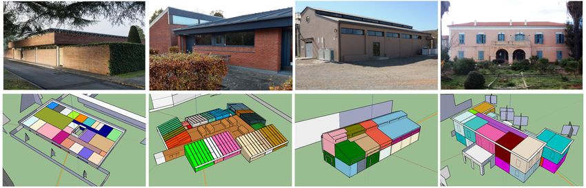
by these variations in the test sites’ building energy demands using detailed BEMs. Figure 5 showsSustainability 2020, 12, 6788 12 of 27
the four test sites analyzed in this study showing a real image from the building and an image of the
performed model in EnergyPlus (in colors for the different thermal zones of each building).
Figure 5. The test sites analyzed. From left to right: office building (University of Navarre, Spain);
Gedved school (Denmark); H2SusBuildand administration building in Lavrio (Greece). On top, the real
buildings and, on the bottom, the building energy models (SketchUp thermal zone representation,
OpenStudio plugin [67]).
The first test site was the office building attached to the Architecture School at the University
of Navarre in Pamplona (Spain). It hosts administration uses and classrooms for the postgraduate
students. This building is a 755 square meter single-story building built in 1974. It has a concrete
structure; the outdoor walls are built of red brick fabric (U value = 0.3 W/m2 K); the flat roof has the
insulation above the deck (U value = 0.2 W/m2 K); and aluminum window frames were installed
in situ with an air chamber. The Gedved public school (Denmark) consists of six buildings and was
built in 1979 and then renewed in 2007. The library of one of the school buildings was selected as the
test site. It is a one-story building with a total surface area of 1138 m2 , with a big central space—the
library—and nine classrooms and serving spaces around it. The building walls consist of two brick
layers with 150 mm insulation in between (U value = 0.27 W/m2 K). The windows are two-layer
double-glazed windows with cold frames. The ceiling is insulated with 200–250 mm mineral wool
for the sloping and flat ceiling, respectively (U value = 0.07 W/m2 K and 0.16 W/m2 K, respectively),
and the floor is made of concrete and contains 150 mm insulation under it (U value = 0.21 W/m2 K).
In Lavrion (Greece), two buildings from the Lavrion Technological and Cultural Park (LTCP) were
used as test sites: H2SusBuild and the administration building. H2SusBuild has a ground floor and an
attic floor with a total surface area of approximately 505 m2 . The ground floor hosts a small kitchen,
toilets, the control room, and the main area. The attic also hosts two offices and a meeting room.
Its envelope consists of a concrete structure with double concrete block walls and single-glazed windows
with aluminum frames. It also has external masonry consisting of double brick walls with 10 cm expanded
polystyrene (EPS) insulation (U value = 0.25 W/m2 K). The roof consists of metallic panels with a 2.5 cm
polyurethane insulation layer in the middle (U value = 0.75 W/m2 K). The administration building hosts
the LTCP managing authority and administrative services. It is a two-story renovated neoclassic building
with a surface area of about 644 m2 . The building envelope is made of stone approximately 70 cm thick
(U value = 1.85 W/m2 K) with wooden-framed double-glazed large windows. The roof consists of a
wooden frame with gutter tiles placed on top (U value = 0.49 W/m2 K).
For each building, an individual pattern of use corresponding to the actual use of the building
was implemented in the simulation model. Each building had its own calendar of use, occupancy,
and internal loads of electric equipment and lighting. Regarding the HVAC systems, setpoints
and usage hours were defined for each. The office building in Pamplona and H2SusBuild and
administration building in Lavrion implemented both heating and cooling systems in the models, and
the Gedved school had only a heating system. Table 2 shows the input data of the four models.Sustainability 2020, 12, 6788 13 of 27
Table 2. Input data of the four models.
Office Building Public School H2SusBuild Administration Building
Pamplona (Spain) Gedved (Denmark) Lavrion (Greece) Lavrion (Greece)
Lighting (W/m2 ) 10 10 8.5 8.5
Equipment (W/m2 ) 8 15 8 8
Occupation schedule Wd 9–21 h/Sat 9–14 h Wd 8–16 h/Sat 8–13 h Wd 9–20 h/Sat 9–14 h Wd 9–20 h/Sat 9–14 h
Heating setpoint (◦ C) 20 Day 21/Night 15.6 21 21
Cooling setpoint (◦ C) 26 No cooling 24 24
Wd: weekdays. Sat: Saturdays.
The results of the statistical analysis for the energy study are presented in Table 3. The table is
divided into four sub-tables, one for each test site. They show the three uncertainty metrics calculated
for the energy demand obtained from simulations using the on-site and third-party weather files (TPW),
with on-site as the reference. The first column of each test site’s table, designated as TPW, shows the
difference in percentage (MADP) of the energy demand when the third-party weather file is used in
the simulation with respect the the reference simulated with on-site weather data. With the inputs
shown in Table 2, the models provide the following annual energy demand: 21.9 kWh/m2 for the office
building, 91.5 kWh/m2 for the Gedved school, 142.2 kWh/m2 for H2SusBuild, and 91.6 kWh/m2 for
the administration building.
The table allows performing two different analyses depending on how it is read. The vertical
interpretation of the table shows the percentage results as a function of the time resolutions (from
annual to hourly criteria) employed for the analysis. On the other hand, horizontally, the variations
in the energy demand for the sensitivity analysis changing only one weather parameter at a time are
presented (DH I, DN I, RH, Temp, WD, and WS).
Table 3. Uncertainty metrics (MADP, CV ( RMSE), and R2 ) were used in the energy analysis for the
four test sites. TPW: the results using the weather file with all the parameters from the third-party
weather data source. The rest changed only one parameter at a time: DH I (diffuse horizontal
irradiation), DN I (direct normal irradiation), RH (relative humidity), Temp (temperature), WD (wind
direction), and WS (wind speed).
Office Building, Pamplona (Spain) School, Gedved (Denmark)
Statistic Index Time TPW DHI DNI RH Temp WD WS TPW DHI DNI RH Temp WD WS
Year 1.42 0.79 4.33 0.50 4.07 0.03 7.95 43.82 0.82 6.24 1.16 0.68 0.01 46.91
Season 9.61 3.93 9.01 3.17 4.07 0.03 11.74 43.82 0.82 6.24 1.16 1.71 0.01 46.91
Month 18.14 4.65 10.29 2.97 12.07 0.03 13.60 43.82 0.82 6.24 1.16 3.59 0.01 46.91
MADP (%)
Week 17.88 5.24 11.17 3.40 14.39 0.04 13.99 43.82 0.90 6.24 1.19 5.16 0.02 46.91
Day 26.03 6.25 11.80 4.02 22.53 0.05 14.08 44.41 0.98 6.25 1.37 8.78 0.02 46.91
Hour 29.96 6.64 12.27 4.71 25.58 0.08 14.31 45.17 1.03 6.27 1.50 10.10 0.02 46.91
Year 1.42 0.79 4.33 0.50 4.07 0.03 7.95 43.82 0.82 6.24 1.16 0.68 0.01 46.91
Season 10.78 4.72 10.11 4.00 4.54 0.03 15.48 58.42 0.95 7.61 1.49 2.25 0.02 60.25
Month 26.12 5.55 13.15 4.02 14.61 0.04 17.96 52.44 0.99 7.05 1.41 4.39 0.02 54.62
CV(RMSE) (%)
Week 26.72 7.12 15.04 5.17 19.68 0.06 20.01 54.15 1.19 7.10 1.45 7.55 0.02 55.29
Day 42.90 9.29 18.18 7.60 34.96 0.08 22.07 60.39 1.44 7.74 1.86 13.11 0.03 59.33
Hour 61.42 13.14 22.37 12.56 50.71 0.20 30.55 91.79 2.75 14.04 3.54 24.99 0.05 88.81
R2 (%) Hour 90.86 99.48 98.64 99.53 92.54 100.00 98.43 95.18 99.99 99.82 99.98 98.55 100.00 96.84
H2SusBuild, Lavrion (Greece) Administration Building, Lavrion (Greece)
TPW DHI DNI RH Temp WD WS TPW DHI DNI RH Temp WD WS
Year 32.86 5.95 5.22 1.97 5.21 1.05 39.40 1.29 11.40 7.27 3.45 9.62 1.93 12.19
Season 44.58 8.14 9.49 3.21 7.25 2.16 39.40 27.75 13.83 13.40 4.20 9.62 2.73 21.63
Month 45.83 10.32 11.20 3.95 11.82 2.94 41.66 38.70 15.56 15.80 4.41 14.73 2.99 29.97
MADP (%)
Week 47.80 10.50 11.15 4.05 13.02 2.93 42.14 38.70 15.69 15.80 4.52 14.78 2.99 29.97
Day 49.46 10.75 11.40 4.46 17.17 2.94 42.49 38.91 15.72 15.80 4.91 16.60 3.00 29.97
Hour 51.58 10.93 11.85 5.12 19.97 2.95 43.95 39.45 15.79 15.83 5.49 17.88 3.01 30.22
Year 32.86 5.95 5.22 1.97 5.21 1.05 39.40 1.29 11.40 7.27 3.45 9.62 1.93 12.19
Season 61.65 9.69 10.71 3.91 12.40 2.58 63.61 36.21 15.57 14.26 4.78 15.61 2.93 34.39
Month 65.24 13.41 13.37 5.04 15.66 3.44 65.89 43.53 20.89 18.63 6.20 20.23 3.83 38.06
CV(RMSE) (%)
Week 72.40 14.11 13.97 5.46 19.34 3.52 73.29 46.18 21.35 19.09 6.62 21.59 3.85 40.61
Day 82.65 14.77 14.74 6.37 24.90 3.68 81.45 49.81 21.93 19.63 7.76 24.17 3.97 43.01
Hour 90.37 18.35 17.92 8.83 34.68 4.85 85.67 90.81 37.52 33.69 15.03 47.91 6.67 72.69
R2 (%) Hour 85.58 98.41 98.43 99.61 93.76 99.88 92.43 81.85 97.30 97.80 99.51 94.91 99.92 91.18Sustainability 2020, 12, 6788 14 of 27
The first analysis obtained from Table 3 was the influence of the time resolution used in the study of
the energy demand variation. In this case, the analysis was done in the vertical from the annual to hourly
criteria. The percentage metrics MADP and CV (RMSE) allowed us to compare the results for each time
grain and study its influence in the results. Both indexes were closely related; however, CV (RMSE) gave
a relatively high weight to large variations. It is remarkable that the differences between CV (RMSE)
and MADP decreased as the time grain increased (from hourly to annual criteria) as, when the energy
demand was accumulated, the outliers were minimized. The results for the hourly basis showed that the
CV (RMSE) values were around twice the MADP values for the four sites and all the weather parameters.
This indicates that significant outliers were present in the energy demand results when both simulations
based on the on-site and third-party weather datasets were compared.
On the other hand, both the MADP and CV ( RMSE) metrics showed how, in the four test sites,
the variations in the energy demand grew as the time grain decreased, which matches with ASHRAE’s
statement about the energy data granularity [44]. If the results were analyzed with the accumulated
energy demand for a period of time (i.e., monthly, annual, etc.), the energy variation was minimized
with respect to the hourly analysis. For example, differences of MADP up to ±38% between the annual
and hourly criteria are seen in the results for the administration building. In this case, the MADP for
the accumulated data for the year was only 1.29%; thus, the annual building energy demand simulated
for the third-party weather file was very similar to the reference, simulated with the on-site weather file.
However, for the hourly basis, this variation grew up to 39.45%, which is a significant deviation.
The reason is because, alternately, in some cases, the model simulation overestimated the energy
demand needed by the building (the model demanded more energy than the reference), and in other
cases, the model underestimated it. When the data were accumulated from the hourly basis to longer
periods of time (daily, weekly, monthly, seasonal, and annual), a compensation effect occurred by
canceling each other out, which resulted in the minimization of the energy demand variation. As the
length of the periods increased, so did the compensation effect and, therefore, also the minimization of
the variations.
It is also remarkable that for all the test sites, the CV ( RMSE) results showed high values for the
monthly and hourly resolutions, which are the time criteria commonly used by the energy analysis standards.
The second analysis was the study of the influence of each weather parameter in the energy demand
variation. In this case, the interpretation of the tables from 3 was done horizontally: the first column
presents the results for the simulation with the third-party weather file (TPW), which had all the weather
parameters changed, and the following columns show the results for the different weather parameters.
Comparing the results of the four test sites using the MADP and CV ( RMSE) indexes, some common
observations can be made. In all of them, the weather parameter that generated less impact in the simulated
energy demand was WD, even though it was the weather parameter that worst fit the on-site weather
data, as was shown in the Taylor diagram (Figure 3). The reason is because the mechanical ventilation and
infiltration EnergyPlus objects used in these models did not account for WD in the simulations [68].
On the other hand, in the four test sites, when WS was analyzed, it showed an important impact
in the energy demand simulations’ outputs. This was mainly due to two causes: The first was the use
of dynamic infiltrations introduced by using the EnergyPlus object ZoneInfiltration:EffectiveLeakageArea,
which took into account the WS parameter in the calculations [68]. The leakage area in cm2 was
calculated by the calibration process previously developed by the authors [69–71]. The second was
because the differences between the third-party WS data and on-site data (see the Taylor diagram in
Figure 3 and the wind roses from Figure 4) were significant.Sustainability 2020, 12, 6788 15 of 27
In both the Gedved school and H2SusBuild, the third-party wind speed provided faster values,
which generated a significant increase in the energy demand during almost all the year, but there were
a few moments with a decrease in the energy demand. Therefore, the compensation effect between the
overestimated and underestimated energy demand was reduced. This explains why the variation due
to WS was high for all the time grains for these test sites. This effect was especially clear in the Gedved
school, which did not have a cooling system. In this case, all the time grains for WS provided the same
MADP because the higher WS of the third-party data always meant a higher heating energy demand
and no energy demand compensation existed.
Regarding the Temp parameter, in the weather data analysis (Section 3.1), based on an hourly
time grain, it was the parameter with less variation between on-site and third-party data for the three
sites. However, the MADP and CV ( RMSE) results, especially for the hourly criteria, showed that it
had a significant impact on the energy demand in the four test sites. It was the second parameter of
influence for the Gedved school, H2SusBuild, and administration building after wind speed and the
first one in the office building with an MADP of ±26%. In relation to the solar irradiation, the Taylor
diagram (Figure 3) showed that DH I from the third-party weather data provided a better correlation
than DN I for the three locations, and this was reflected in the sensitivity energy analysis. For the
Gedved school, these two parameters had less impact on the energy demand than for the other three
models. The reason is because the school lacked a cooling system; therefore, in summer, when more
solar access was available, no energy demand was taken into account.
To conclude the explanation of Table 3, factor R2 was analyzed. It compared the shape of the
energy demand curves from the different simulations and showed that the energy demand simulated
with the third-party weather data fit quite well with the energy demand simulated from the on-site
data for the four test sites (with R2 between ±82% and ±95%). Regarding the different weather
parameters, the results for each parameter matched with the analysis of the hourly percentage indexes.
The parameters with lower hourly MADP and CV ( RMSE) values had higher R2 values.
Finally, to show in a visual way the previous analysis of the influence of the time resolution
employed in the study and the sensitivity of each weather parameter, the MADP index results are
plotted in Figure 6. Each graph presents the MADP result for each test site. In the graphs, the six
time resolutions are shown on the x axis, and the dashed line presents the results for the simulation
with all the third-party weather parameters (TPW). Each color represents the results for each weather
parameter of the sensitivity analysis. The graphs show how the variations in the energy demand grew
as the time grain decreased, especially Temp. They also show that WS was the most sensitive weather
parameter for the Gedved school, H2SusBuild, and administration building. Only in the case of the
office building in Pamplona was WS the most sensitive weather parameter taking into account an
annual criterion; however, per hour, it changed to Temp.
Previous analyses showed the significant variations in the energy demand when using different
actual weather datasets. In order to study if these differences in the energy demand were mostly due
to the building architectures or to the weather, a complementary theoretical analysis was performed,
and this is presented in the following section.
3.2.1. Analysis of the Buildings’ Architecture Influence on the Energy Results
Since four test sites were available for this research, a complementary study was performed to
analyze the influence of the building’s architecture on the previous energy results. The four buildings,
which were completely different in terms of the materials, construction systems, thermal mass,
and window-to-wall ratio, were simulated with the same weather data (on-site and third-party weather
files). For this study, we selected the most homogeneous weather when comparing the third-party
to the on-site weather data: as shown in the previous analysis, energy demands are very sensitive
to WS, so the Gedved weather was discarded for this analysis because its WS was the one with the
worst fit to the reference (see Figure 3). Temp was also a sensitive parameter, and the three weathers
had similar statistical metrics. Finally, for the solar radiation parameters DH I and DN I, Pamplona’sSustainability 2020, 12, 6788 16 of 27
weather better matched the reference compared to Lavrion. Therefore, the Pamplona weather file was
chosen to develop this theoretical study, and for this reason, the four models were configured to have
the same internal loads, HVAC systems, and schedules as the Pamplona office building.
Figure 7 shows the MADP results for this study. The two graphs on the top present the results
using the third-party weather file, which had all the weather parameters provided by the weather
service. They show how when the test sites were simulated with their own weather files (graph on
the left), the MADP results and the trend of the curve were very different for the four test sites (each
colored line represents one test site). However, when the test sites were simulated with Pamplona’s
weather file (graph on the right with dashed lines), the curves became very similar, reducing the
differences in the MADP values and in the trend of the curve.
Thus, the main value responsible for the variation in the energy demand was the weather dataset
employed in the simulations and not the building’s characteristics. This effect was also reflected in
the results from the sensitivity analysis, which are also presented in Figure 7 for the Temp, DN I, DH I,
and WS parameters. The curves from the graphs on the right, which are the simulations of all the test
sites with Pamplona’s weather file, were very similar compared to the curves from the graphs on the
left, especially in the case of wind speed. This study demonstrated the great influence of the weather
parameters on the variation of the building’s energy demand, almost independently of the model,
and this showed the importance of the selection of the weather dataset used in the BEM simulations.
Office building (Pamplona) School (Gedved)
50 Third-party weather 50
Temperature
Relative humidity
40 Direct normal irradiation 40
Diffuse horizontal irradiation
MADP (%)
MADP (%)
Wind speed
30 30
Wind direction
20 20
10 10
0 0
Year Season Month Week Day Hour Year Season Month Week Day Hour
Time grain Time grain
H2SusBuild (Lavrion) Administration building (Lavrion)
50 50
40 40
MADP (%)
MADP (%)
30 30
20 20
10 10
0 0
Year Season Month Week Day Hour Year Season Month Week Day Hour
Time grain Time grain
Figure 6. Representation of the MADP (%) of the energy demand analysis for the four test sites and
for the different time grains. The dashed black line represents the results using the weather file with all
the third-party weather parameters. Each colored line represents each one of the weather parameter
results from the sensitivity analysis.Sustainability 2020, 12, 6788 17 of 27
SIMULATION OF EACH SITE SIMULATION OF ALL THE SITES
WITH ITS WEATHER FILE WITH PAMPLONA'S WEATHER FILE
50 50 Office building
School
H2SusBuild
THIRD-PARTY WEATHER
40 40 Administration building
Sensitivity analysis:
MADP (%)
MADP (%)
30 30
20 20
10 10
0 0
Year Season Month Week Day Hour Year Season Month Week Day Hour
Time grain Time grain
50 50
40 40
Sensitivity analysis:
TEMPERATURE
MADP (%)
MADP (%)
30 30
20 20
10 10
0 0
Year Season Month Week Day Hour Year Season Month Week Day Hour
Time grain Time grain
50 50
DIRECT NORMAL IRRADIATION
40 40
Sensitivity analysis:
MADP (%)
MADP (%)
30 30
20 20
10 10
Year Season Month Week Day Hour Year Season Month Week Day Hour
Time grain Time grain
DIFFUSE HORIZONTAL IRRADIATION
50 50
40 40
Sensitivity analysis:
MADP (%)
MADP (%)
30 30
20 20
10 10
0
Year Season Month Week Day Hour Year Season Month Week Day Hour
Time grain Time grain
50 50
Sensitivity analysis:
40 40
WIND SPEED
MADP (%)
MADP (%)
30 30
20 20
10
10
Year Season Month Week Day Hour Year Season Month Week Day Hour
Time grain Time grain
Figure 7. The comparison between the simulation results when each test site was simulated with its
weather (on the left with continuous lines) and when all the test sites were simulated with Pamplona’s
weather (on the right with dashed lines). Each color represents a test site. The graphs show the MADP
for the energy demand for the different temporal resolutions. From above to below are shown: results
when the third-party weather file was used (all the parameters were changed in the weather file) and
the sensitivity analysis results for temperature, direct normal irradiation, diffuse horizontal irradiation,
and wind speed.You can also read