Interactive Data Exploration Using Semantic Windows
←
→
Page content transcription
If your browser does not render page correctly, please read the page content below

Interactive Data Exploration Using
                                                Semantic Windows

                      Alexander Kalinin                                         Ugur Cetintemel                           Stan Zdonik
                          Brown University                                         Brown University                      Brown University
                akalinin@cs.brown.edu                                       ugur@cs.brown.edu                        sbz@cs.brown.edu

ABSTRACT
We present a new interactive data exploration approach,
called Semantic Windows (SW), in which users query for
multidimensional “windows” of interest via standard DBMS-
style queries enhanced with exploration constructs. Users
can specify SWs using (i) shape-based properties, e.g., “iden-
tify all 3-by-3 windows”, as well as (ii) content-based proper-
ties, e.g., “identify all windows in which the average bright-
ness of stars exceeds 0.8”. This SW approach enables the                                        Figure 1: Exploration queries searching for bright
interactive processing of a host of useful exploratory queries                                  star clusters (left) and periods of high average stock
that are difficult to express and optimize using standard                                       prices (right). Some results are highlighted.
DBMS techniques.
   SW uses a sampling-guided, data-driven search strategy to                                    Unfortunately, traditional DBMSs are designed and opti-
explore the underlying data set and quickly identify windows                                    mized for supporting neither interactive operation nor ex-
of interest. To facilitate human-in-the-loop style interactive                                  ploratory queries. Users typically have to write very com-
processing, SW is optimized to produce online results dur-                                      plex queries (e.g., in SQL), which are hard to optimize and
ing query execution. To control the tension between online                                      execute efficiently. Moreover, users often have to wait until
performance and query completion time, it uses a tunable,                                       a query finishes without getting any intermediate (online)
adaptive prefetching technique. To enable exploration of big                                    results, which is often sufficient for exploratory purposes.
data, the framework supports distributed computation.                                             Consider the following data exploration framework. A
   We describe the semantics and implementation of SW as                                        user examines a multidimensional data space by posing a
a distributed layer on top of PostgreSQL. The experimental                                      number of queries that find rectangular regions of the data
results with real astronomical and artificial data reveal that                                  space the user is interested in. We call such regions windows.
SW can offer online results quickly and continuously with                                       After getting some results, the user might decide to stop the
little or no degradation in query completion times.                                             current query and move to the next one. Or she might want
                                                                                                to study some of the results more closely by making any of
Categories and Subject Descriptors                                                              them the new search area and asking for more details. Let
                                                                                                us look at two illustrative examples in Figure 1.
H.2.4 [Database Management]: Systems—query process-
ing                                                                                                Example 1. A user wants to study a data set containing
                                                                                                information about stars and other objects in the sky (e.g.,
Keywords                                                                                        SDSS [1]). She wants to find a rectangular region in the sky
                                                                                                satisfying the following properties:
Data exploration; Query processing                                                               • The shape of the region must be 3◦ by 2◦ , assuming an-
                                                                                                   gular coordinates (e.g., right ascension and declination).
1.      INTRODUCTION                                                                             • The average brightness of all stars within the region must
  The amount of data stored in database systems has been                                           be greater than 0.8.
constantly increasing over the past years. Users would like
                                                                                                  The example above describes a spatial exploration case,
to perform various exploration tasks with interactive speeds.
                                                                                                where windows of interest correspond to two-dimensional
Permission to make digital or hard copies of all or part of this work for personal or           regions of the sky. However, the framework can be used for
classroom use is granted without fee provided that copies are not made or distributed           other cases, e.g., for one-dimensional time-based data:
for profit or commercial advantage and that copies bear this notice and the full citation
on the first page. Copyrights for components of this work owned by others than the                 Example 2. A user studies trading data for some com-
author(s) must be honored. Abstracting with credit is permitted. To copy otherwise, or          pany. The search area represents stock values over a period
republish, to post on servers or to redistribute to lists, requires prior specific permission   of time. The user wants to find a time interval (i.e., a one-
and/or a fee. Request permissions from permissions@acm.org.                                     dimensional region) having the following properties:
SIGMOD’14, June 22–27, 2014, Snowbird, UT, USA
                                                                                                 • The interval must be of length from 1 to 3 years.
Copyright is held by the owner/author(s). Publication rights licensed to ACM.
ACM 978-1-4503-2376-5/14/06 ...$15.00.
                                                                                                 • The average of stock prices within the interval must be
http://dx.doi.org/10.1145/2588555.2593666.                                                         greater than 50.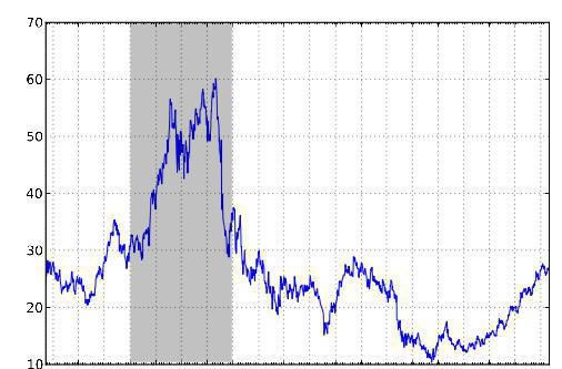
By defining windows of interest in terms of their desired      trees or R-trees. To estimate utilities we collect a sample of
properties, users can express a variety of exploration queries.   the data offline and store it in the DBMS.
Such properties, which we call conditions, can be specified          We conducted an experimental evaluation using synthetic
based on the shape of a window (e.g., the length of a time        and real data. For the latter we used SDSS [1]. The experi-
interval) and an aggregate function of the data contained         mental results show that in many cases our framework can
within (e.g., the average stock value within an interval).        offer online results quickly and continuously, outperform-
   Traditional SQL DBMSs cannot deal with the type of             ing traditional DBMSs significantly. For the comparison we
queries presented here in an efficient and compact way. Avail-    used a complex SQL query, mentioned above, and query
able constructs, such as GROUP BY and OVER, do not allow          completion time of SW queries is often better. Due to the
users to define and explore all valid windows. Although it is     complexity of the query, the query processor was not able
possible to express such queries with a SQL query involving       to plan and execute it efficiently. However, even when the
a number of recursive Common Table Expressions (CTEs),            framework performs worse in total time, the difference can
such a query would be difficult to optimize due to its com-       be eliminated or significantly reduced by prefetching.
plexity.                                                             In summary, the proposed SW framework:
   Another important requirement in data exploration is in-        • Allows users to interactively explore data in terms of
teractivity. Since the amount of data users have to explore           multidimensional windows and select interesting ones via
is generally large, it is important to provide online results.        shape- and content-based predicates.
This allows the user to interrupt the query and modify it          • Provides online results quickly, facilitating human-in-the-
to better reflect her interests. Moreover, many applications          loop processing needed for interactive data exploration.
can be satisfied with a subset of results, without the need        • Uses a data-driven search algorithm integrated with strat-
to compute all of them. Most SQL implementations do not               ified sampling, adaptive prefetching and data placement
allow such functionality, making users wait for results until         to offer interactive online performance without sacrificing
the entire query is finished.                                         query completion times.
   Our approach treats an exploration query as a data-driven       • Offers a diversification approach that allows users to di-
search task. The search space consists of all possible win-           rect the search for qualifying SWs in unexplored regions
dows, which can vary in size and overlap. We use a cost-              of the search space, thus allowing the user to control the
benefit analysis to quantify a utility measure to rank the            classical exploration vs. exploitation trade-off.
windows and decide on the order by which we will explore           • Provides an efficient distributed execution framework that
them. We use sampling to estimate values for conditions on            partitions the data space to allow parallelism while effec-
the data, which allows us to compute a distance from these            tively dealing with partition boundaries.
values to the values specified in the query. We then guide           The remainder of the paper is organized as follows. Sec-
the search using a utility estimate, which is a combination of    tion 2 gives a formal description of the framework. Section
this distance, called benefit, and the cost of reading the cor-   3 describes extensions for SQL to support SW queries. Sec-
responding data from disk. We use shape-based conditions          tion 4 gives a description of the algorithm and our prefetch-
to prune parts of the search space.                               ing technique. Section 5 talks about the architecture and
   Since logical windows may not correspond to the physical       implementation details. Section 6 provides results of the
placement of data on disk, reading multiple dispersed win-        experimental evaluation. Section 7 reviews related work.
dows may result in a significant I/O overhead. The overhead       Section 8 concludes the paper.
comes from seeks and reading the same data pages multiple
times. Thus there is a tension between online performance         2.    SW MODEL AND QUERIES
and query completion time. To control this tension, we use a
                                                                      Assume a data set S containing objects with attributes
prefetching technique: by prefetching additional data when
                                                                  a1 , . . . , am (e.g., brightness, price, etc.) and coordinates
reading a window and thus decreasing the number of dis-
                                                                  x1 , . . . , xn . Thus, S constitutes an n-dimensional search
persed reads, it is possible to reduce the overhead and fin-
                                                                  area with dimensions d1 , . . . , dn . We will often specify S in
ish the query faster. However, this approach might result
                                                                  terms of the intervals it spans (e.g., S = [L1 , U1 ) × [L2 , U2 )
in worse online performance, since delays for online results
                                                                  for a two-dimensional data set). Next, we define a grid
might increase. To manage this trade-off, we use an adap-
                                                                  on top of S. The grid GS is defined as a vector of steps:
tive prefetching algorithm that dynamically adjusts the size
                                                                  (s1 , s2 , . . . , sn ). It divides each interval [Li , Ui ) into disjoint
of prefetching during execution. While new results are being
                                                                  sub-intervals of size si , starting from Li : [Li , Li + si ) ∪ [Li +
discovered, we prefetch less to keep delays to a minimum.
                                                                  si , Li + 2si ) ∪ · · · ∪ [Li + k · si , Ui ). The last sub-interval
When no new results can be found, we start to prefetch more
                                                                  might have size less than si , which has no impact on the
to speed up the execution and finish the query faster. Ad-
                                                                  discussion. Thus, S is divided into a number of disjoint
ditionally, we allow users to control the prefetching strategy
                                                                  cells. The search space of an SW query consists of all pos-
to favor one side of the trade-off or the other.
                                                                  sible windows. A window is a union of adjacent cells that
   Our new framework, which we call Semantic Windows
                                                                  constitutes an n-dimensional rectangle. Since the grid de-
(SW), can be implemented as a layer on top of existing
                                                                  termines the windows available for exploration, the user can
DBMSs. For experimentation purposes, we implemented a
                                                                  specify a particular grid for every query.
distributed version of the framework on top of PostgreSQL.
                                                                      Let us revisit examples presented in the Introduction. Ex-
The computation is done by multiple workers residing on
                                                                  ample 1 could be represented as follows:
different nodes, which interact between themselves and with
                                                                   • d1 = ra, d2 = dec, a1 = brightness 1 .
the DBMS via TCP/IP. To explore windows efficiently, we
                                                                   • S = [100◦ , 300◦ ) × [5◦ , 40◦ ), GS = (1◦ , 1◦ ).
require efficient execution of multidimensional range queries,
                                                                      and Example 2 as:
which can be achieved via common index structures, like B-
                                                                   • d1 = time, a1 = price.
• GS = (1 year), S = [1999/02/01, 2003/11/30) SELECT LB(ra), UB(ra), LB(dec), UB(dec),
An objective function f (w) is a scalar function, defined AVG(brightness)
for window w. There are two types of objective functions: FROM sdss
• Content-based. They are computed over objects belong- GRID BY ra BETWEEN 100 AND 300 STEP 1,
ing to the window. Since the value must be scalar, this dec BETWEEN 5 AND 40 STEP 1
type is restricted to aggregates (average, sum, etc). We HAVING AVG(brightness) > 0.8 AND
further restrict them to be distributive and algebraic [6]. LEN(ra) = 3 AND
This is done for efficiency purposes — the value of f (w) LEN(dec) = 2
must be computable from the corresponding values of the
cells in w. We discuss this in more detail in Section 5.
• Shape-based. They describe the shape of a window and do Figure 2: An SW query written with the proposed
not depend on data within the window. We restrict our- SQL extensions
selves to the following functions: card(w) and lendi (w).
The former defines the number of cells in w, which we example, we provide experimental results for PostgreSQL
call the cardinality of w. The latter is the length of w in in Section 6. More importantly, the query performs an ag-
dimension di in cells. Assuming w spans interval [li , ui ) gregation in the beginning. This means the computation is
in di , lendi (w) = uis−l
i
i
. Other functions, for example blocked until all cells have been computed. Such a query
computing the perimeter or area, are possible. would not be able to output online results. Techniques like
A condition c is a predicate involving an objective func- online aggregation [8] are very limited here, since exact, not
tion. The result of computing condition c for window w approximate, results are required. Also, applying online ag-
is denoted as wc . The framework is restricted to algebraic gregation to such a complex query is challenging at best.
comparisons, for example f (w) > 50. To address these problems we propose to extend SQL to
The conditions for Example 1 can be defined as: lenra (w) = directly express SW queries. Our extensions are as follows:
3, lendec (w) = 2 and avg brightness(w) > 0.8. For Exam- • The new GRID BY clause for defining the search space.
ple 2, the conditions can be expressed as: lentime (w) ≥ 1, This clause replaces GROUP BY (both cannot be used at
lentime (w) ≤ 3 and avg price(w) > 50. the same time).
An SW query can now be defined as QSW = {S, GS , C}, • New functions that can be used for describing windows.
where C is a set of conditions. The result of the query is Namely, LB(di ), U B(di ) to compute the lower and upper
defined as: RESQ = {w ∈ WS |∀c ∈ C : wc = true}, where boundaries of a window in dimension di . Other functions
WS is a set of all windows, defined by GS . are possible depending on the user’s needs.
• New functions for defining shape-based conditions. Namely,
LEN (di ), which is equivalent to lendi (w). This function
3. EXISTING SQL EXTENSIONS FOR DATA is syntactic sugar, since it is possible to compute it by
EXPLORATION using boundary functions introduced above.
As a first option, we look into expressing SW queries using Additionally, we reuse the existing SQL HAVING clause to
SQL. While SQL has constructs for working with groups of define conditions for the query. Figure 2 shows how Example
tuples, such as GROUP BY and OVER, they are insufficient for 1 can be expressed with the proposed extensions.
expressing all possible windows. GROUP BY does not allow In the GRID BY clause, BETWEEN defines the boundaries of
overlapping groups, which makes it impossible to express the search area for every dimension and STEP defines steps
overlapping windows. OVER allows users to study a group of the grid (ra, dec are attributes of sdss and serve as di-
of tuples (also called window in SQL) in the context of the mensions). The query is processed in the same way as a
current tuple via PARTITION BY clause. However, it allows GROUP BY query in SQL, except that instead of groups it
only one such a group for every tuple, not a series of groups works with windows defined via the GRID BY clause. HAVING
with different shapes. Thus, only a subset of possible win- has the same meaning — filtering windows that do not sat-
dows can be expressed this way. The standard SQL is even isfy conditions. Since SELECT outputs windows, only func-
more restrictive and does not allow functions to be used tions describing a window can be used there: the ones de-
in PARTITION BY. This makes it difficult to express multidi- scribing the shape and the ones that were used for defin-
mensional windows at all. ing conditions. Similar restrictions are imposed in the SQL
One general way, which we implemented, is to express an standard for GROUP BY queries.
SW query as follows:
1. Compute objective function values for every cell of the 4. THE SW FRAMEWORK
grid via GROUP BY.
2. Generate every possible window by combining cells, using 4.1 Data-Driven Online Search
recursive CTEs. Values for the objective functions are We first describe our basic algorithm for executing SW
computed by combining the values of the cells. queries with online results. Logically, the search process can
3. Filter windows that do not satisfy the conditions. be described as follows:
This type of query leads to two major problems. First, due 1. Data set S is divided into cells ci as specified by grid GS .
to its complexity most traditional query optimizers would 2. All possible windows w are enumerated and explored one
likely have hard time executing the query efficiently. As an by one in an arbitrary order.
1
The original SDSS data does not contain a brightness at- 3. If window w satisfies all conditions (i.e., {∀c ∈ C : wc =
tribute. However, this attribute or a similar one can be true}), the window belongs to the result.
computed from other attributes using an appropriate func- This suggests a naive algorithm to compute an SW query.
tion. The algorithm presented in this section is designed to pro-vide online results in an efficient way. The main idea is to estimations. In this case only the windows for which new
dynamically generate promising candidate windows as the data is available are actually updated.
search progresses and explore them in a particular order. The procedure begins by determining the initial windows
The search space of all possible windows is structured as via the StartW indows() function. Since the search space
a graph. First we define relationships between windows. might be large, it is important to aggressively prune win-
Giving a window w, an extension of w is a window w0 , which dows. Suppose the user specifies a shape-based condition
is constructed by combining cells of w with a number of that defines the minimum length n for resulting windows in
adjacent cells from its neighborhood. If w0 is extended in a some dimension (e.g., lendi (w) ≥ n). StartW indows() does
single dimension and direction from w, it is called a neighbor. not generate windows that cannot satisfy this condition, ef-
An example can be seen in Figure 3. A two-dimensional fectively pruning initial parts of the graph. Otherwise, the
search area is divided into four cells, labeled 1 through 4. search starts from cells. A similar check is made in the
Window 1|2|3|4 2 is an extension of window 1, since it is GetN eighbors() function, which generates all neighbors of
produced by adding adjacent cells 2 through 4. At the same the current window. It checks for conditions that specify the
time, 1|2|3|4 is a neighbor of 1|2, since 1|2 is extended only maximum length in a dimension (e.g., lendj (w) ≤ m) and
in the vertical dimension and the only direction — “down”. does not generate neighbors that violate such conditions.
The resulting search graph consists of vertices representing Since the number of windows can be very large, at some
windows and edges connecting neighbors. point the priority queue may not fit into memory. It is
With the search graph defined, we use a heuristic best-first possible to spill the tail of the queue into disk and keep only
search approach to traverse it. The heuristic is based on the its head in memory. When a new window has a low utility,
utility of a window, which will be discussed in more detail it is appended to the tail (in any order). When the head
in Section 4.2. In a nutshell, utility is a combination of the becomes small enough, part of the tail is loaded into memory
cost of reading a window from disk and the potential benefit and priority-sorted, if needed. For efficiency, the tail can
of the window, which is a measure of how likely the window be separated into several buckets of different utility ranges
is to satisfy the query conditions. The resulting algorithm where windows inside a bucket have an arbitrary ordering.
is presented as pseudo-code below: While additional pruning, based on other conditions, might
further increase the efficiency of the algorithm, it is not safe
Algorithm 1 Heuristic Online Search Algorithm to apply in general. Since providing approximate results
is not an option we consider, it is not possible to discard
Input: search space S, grid GS , conditions C
a window or its extensions solely on the basis of estima-
Output: resulting windows RESQ
tions. Content-based conditions must be checked on the
exact data. In general, extensions have to be explored as
procedure HeuristicSearch(S, GS , C)
well, since they too can produce valid results. However, in
P Q ← ∅, RESQ ← ∅ . PQ — priority queue
some restricted cases, it is possible to prune them.
StartW ← StartW indows(S, GS , C)
One example is the so-called anti-monotone constraints
for all w ∈ StartW do
[9]. In case of a content-based condition sum(w) < 10 and
EstimateU tility(w)
assuming sum() can produce only non-negative values, it
insert(P Q, w) . utility as priority
is possible to prune all windows that contain the current
while ¬empty(P Q) do window w0 if sum(w0 ) ≥ 10, since sum() is monotonic on
w ← pop(P Q) the size of a window. The length and cardinality of a window
U pdateU tility(w) are other examples of such functions. Since they are data-
if U tility(w) ≥ U tility(top(P Q)) then independent, the corresponding conditions are always safe to
Read(w) . read from disk if needed use for pruning, which our algorithm supports. Such anti-
U pdateResult(RESQ , C, w) monotone pruning, however, would not necessarily decrease
N ← GetN eighbors(w, S, GS ) the amount of data that has to be read. Windows that just
for all n ∈ N do overlap with w0 might still be valid candidates for the result.
EstimateU tility(n)
insert(P Q, n) 4.2 Computing Window Utilities
else The utility of a window is a combination of its cost and
insert(P Q, w) benefit. The cost determines how expensive it is to read a
window from disk. Since the grid is defined at the logical
The algorithm uses a priority queue to explore candidate level without considering the underlying data distribution,
windows according to their utilities. The utility is estimated some windows may be more expensive to read than others,
before a window is read from disk via a precomputed sample. if the data distribution is skewed. Also, since windows over-
Since estimations might improve while new data is read from lap, the cost of a window may decrease during the execution
disk during the search, when the next window is popped if some of its cells have already been read as parts of other
from the queue, we update its utility via the U pdateU tility() windows. We assume that the system caches objective func-
function. This can be seen as lazy utility update. If the win- tion values for every cell it reads, so it is not necessary to
dow still has the highest utility, it is explored (i.e., read from read a cell multiple times. The cost is computed as follows.
disk and checked for satisfying the conditions). Otherwise, Let |S| = n, |GS | = m, where |S| is the total number of
it is returned to the queue to be explored later. Addition- objects in the data set and |GS | is the total number of cells.
ally, we periodically update the whole queue to avoid stale Let the number of objects belonging to non-cached cells of
window w be |w|nc . Then the cost Cw of the window is
2
c1 | . . . |ck labels a window consisting of cells c1 through ck computed as: Cw = |w| nc
n/m
= |w|nc
n
m
.In case data does not have considerable skew, the cost
is approximately equal to the number of non-cached cells
belonging to the window. However, in general the cost might
differ significantly, depending on the skew. To compute the
cost accurately, it is necessary to estimate the number of
objects in a window. We use a precomputed sample for the
initial estimations and update these estimations during the
execution as we read data. When reading a window, we
not only compute the objective function values, but also the
number of objects for every cell. This results in computing
an additional aggregate for the same cells, which does not
incur any overhead. Figure 3: The search graph for an SW query, an-
The second part of the utility computation is benefit esti- notated with benefits, costs, utilities and objective
mation. Here, we determine how “close” a window is to sat- function estimations
isfying the user-defined conditions. First, we compute the
benefit for every condition independently. The framework (bottom) of windows specify benefits, costs and utilities as
currently supports only comparisons as conditions, but the b, c and u respectively. Initially, only the values for cells are
approach can be generalized for other types of predicates. computed, and the values for other windows are computed
Assume an objective function f (w) and the corresponding when they are explored. The search progresses as follows:
condition in the form: f (w) op val, where op is a compari- 1. Since there are no shape-based conditions, the search
son operator. We assume f (w) can be estimated for window starts with cells. Initially, P Q = [2, 3, 1, 4], and the algo-
w via the precomputed sample. Let the estimated value be rithm picks cell 2, which is read from disk. It generates
fw . Then the benefit bfw for condition f for window w is two neighbors: 1|2 and 2|4. f (w) is estimated from the
computed as follows: sample, and the windows are put into the queue. Note
n o that C1|2 = C1 = 1, C2|4 = C4 = 2, since cell 2 has
already been read.
(
f max 0, 1 − |fweps
−val|
if fw op val = f alse
bw = 2. P Q = [3, 1|2, 1, 2|4, 4]. The algorithm picks cell 3 and
1 if fw op val = true reads it from disk. It generates its neighbors: 1|3 and
3|4.
The value eps determines the precision of the estimation
3. P Q = [1|3, 1|2, 1, 2|4, 3|4, 4]. The next window to explore
and is introduced to normalize the benefit value to be be-
is 1|3. It is processed in the same way and generates the
tween 0 and 1. It often can be determined for a particu-
only neighbor possible — 1|2|3|4.
lar function based on the distance of the corresponding at-
4. P Q = [1|2, 1, 1|2|3|4, 2|4, 3|4, 4]. The search moves to
tribute values from val. For example, if f = avg(ai ), then
window 1|2. Since cells 1 and 2 have already been read,
max{|val − min(ai )|, |val − max(ai )|} can serve as eps. Al-
the window is not read from disk and explored in mem-
ternatively, a value of the magnitude of val can be taken
ory. Its only extension, 1|2|3|4, was generated already
initially and then updated as the search progresses.
and is skipped.
The total benefit Bw of window w is computed as the
5. P Q = [1, 1|2|3|4, 2|4, 3|4, 4]. The search then goes through
minimum of the individual benefits, since a resulting window
1, 1|2|3|4, 2|4, 3|4 and, finally, 4 in the order of their
must satisfy all conditions: Bw = minf ∈C bfw .
utilities. Due to caching, all windows except 1|2|3|4 are
Since bfw ∈ [0, 1], it follows that Bw ∈ [0, 1]. The utility of
checked in memory, and when 1|2|3|4 is explored, only
window w is a combination of the benefit and cost:
cell 4 is read from disk.
Cw At every step, after a window is read from disk, the con-
Uw = sBw + (1 − s) 1 − min ,1 dition is checked. If the window satisfies the condition, it is
k
output to the user. Otherwise, it is filtered.
The cost is divided by k to normalize it to [0, 1]. In case
the user did not provide any restrictions on the maximum
cardinality for windows, k is equal to m. Otherwise, it is 4.3 Progress-driven Prefetching
equal to the maximum possible cardinality inferred from Reconsider the heuristic search algorithm presented in
shape-based conditions. The parameter s (s ∈ [0, 1]) is the Section 4.1. Every time a window is explored, all of its cells
weight of the benefit. Lowering the value allows exploring that do not reside in the cache have to be read from disk. If
cheaper, but promising, windows first, while increasing it the grid contains a large number of cells, the search process
prioritizes windows with higher benefits at the expense of might perform a large number of reads, which might incur
the cost. Intuitively, it is better to first explore windows considerable overhead. If the data placement on disk does
with high benefits and use the cost as a tie-breaker, picking not correspond to the locality implied by windows, reading
the cheaper window when benefits are close to each other. even a single window might result in touching a large num-
We illustrate the algorithm with the search graph from the ber of pages dispersed throughout the data file. The problem
previous section, presented in Figure 3. The exact param- goes beyond disk seeks. If only a small portion of objects
eters for the search area are irrelevant. Assume the whole from each page belongs to the window, these pages have
data set contains n = 200 objects and the number of ob- to be re-read later when other windows touch them. This
jects in cells 1, 2, 3 and 4 (m = 4) is 50, 20, 30 and 100 might create thrashing. An implementation of the algorithm
respectively. We assume that eps = 10, k = 4 and s = 21 . that does not modify the database engine cannot deal with
The only condition is f (w) > 13 and the estimated values this problem. The problem might be partially remedied by
fw are specified on top of windows. The numbers to the left clustering the data, yet there are times when users cannotchange the placement of data easily. The ordering might Algorithm 2 Prefetch Algorithm
be dictated by other types of queries users run on the same Input: window w, prefetch size p
data. Another possible way is to materialize the grid by pre- Output: window to read w0
computing all cells. However, this requires that the query
parameters (i.e., the search area, the grid and functions) be procedure Prefetch(w, p)
known in advance. Since exploration can often be an unpre- w0 ← w
dictable ad hoc process, we assume the parameters may vary for i = 1 → n do . n — number of dimensions
between queries. In this case, materialization performed for for dir ∈ {lef t, right}
Q do
every query will make online answering impossible. max ← Cw0 + p k6=i lendk (w0 )
To address this problem, we use an adaptive prefetch- repeat
ing strategy. Our framework explores windows in the same ext ← GetN eighbor(w0 , di , dir)
way, but it prefetches additional cells with every read. The if Cext ≤ max then
window is extended to a new window, according to the def- w0 ← ext
inition of the extension from Section 4.1. When the size until Cext > max
of prefetching increases, intermediate delays might become
more pronounced due to the additional data read with every
can be found. This allows us to finish the query faster. We
window. At the same time, due to the decreased number of
assume that the number of consecutive false positives due
reads, this reduces the overhead and the query completion
to sampling errors is not going to be large, so online perfor-
times. Decreasing the size of prefetching has the opposite ef-
mance will not suffer.
fect. While this approach can be seen as offering a trade-off
The pseudo-code of Algorithm 2 describes how a window
between the online performance and query completion time,
is extended according to the value of p. The size defines a
we show that, in some cases, prefetching can be beneficial
“cost budget” for the extension. This budget is applied as a
for both, as we demonstrate through experiments.
number of possible extension cells independently for every
During the search it is beneficial to dynamically change
direction in every dimension. The budget-based approach
the size of prefetching. A read can have two outcomes. Posi-
allows us to address a possible data skew. Since for a fixed
tive reads result in reading cells that belong to the resulting
dimension a window can be extended in two directions, we
windows. It might be the window just read or windows
denote them as lef t and right.
overlapping with it. While new results keep coming, the
framework prefetches a constant default amount, controlled
by a parameter. By setting this parameter users can favor 4.4 Diversifying Results: Exploration vs. Ex-
a particular side of the trade-off. On the other hand, a false ploitation
positive read does not contribute to the result, reading cells
Our basic SW strategy is designed for “exploitation” in
that do not belong to the resulting windows. A false positive
that it is optimized to produce qualifying SWs as quickly
can happen for two reasons:
as possible without taking into account what parts of the
• The remaining data does not contain any more results.
underlying data space these results may come from. In many
To confirm this, the search process still has to finish read-
data exploration scenarios, however, a user may want to
ing the data. All remaining reads are going to be false
get a quick sense of the overall data space, requiring the
positives. In this case the best strategy would be to read
underlying algorithm to efficiently “explore” all regions of
it in as few requests as possible.
the data, even though this may slow down query execution.
• Due to sampling errors, utilities might be estimated in-
With the basic algorithm, when a number of resulting
correctly. Since new results are still possible, it is better
windows is output, other promising windows that overlap
to continue reading data via select, short requests.
with them will have reduced costs and higher utilities due
Since it is basically impossible to distinguish between the
to the cached cells. Such windows will be explored first,
two cases without seeing all the data, we made the prefetch-
which might favor results located close to each other. In
ing strategy adapt to the current situation. In this new
some cases it might be desirable to jump to another part of
technique, which we refer to as progress-driven prefetching,
the search space that contains promising, but possibly more
the size of prefetching increases with every new consecutive
expensive, windows. This way the user might get a better
false positive read, which addresses the first case. When a
understanding of the search area and results it contains. We
positive read is encountered, the size is reset to the default
considered two approaches to achieve that.
value to switch back at providing online results. The size of
The first approach is to include a notion of diversity of
prefetching, p, is computed as:
results within the utility computation. We define a clus-
p = (1 + α)α+f p reads − 1 ter of results as an MBR (Minimum Bounding Rectangle)
containing all resulting windows that overlap each other.
α ≥ 0 is the parameter that controls the default prefetch- Discovering all final clusters faster might give a better un-
ing size. We call it the aggressiveness of prefetching. In case derstanding of the whole result. When a new window is
α = 0, p = 0 and no additional data is read. Increasing α re- explored we compute the minimum Euclidean distance dist
sults in increasing the default prefetching size, which favors from the window to the clusters already found. The distance
the query completion time. f p reads is the number of con- is normalized to [0, 1] and included as a part of the window’s
0
secutive false positives. When it increases, p increases expo- benefit: Bw = Bw +dist
2
, resulting in the modified utility Uw0 .
nentially. If a new result is discovered, f p reads is set to 0, If the window being explored belongs to a cluster, we find
and p is automatically reset. This corresponds to the adapt- the next highest-utility window w0 with a non-zero dist and
able strategy described above. The exponential increase was compare utilities Uw0 and Uw0 0 . If w0 has a higher utility,
chosen so that the size would grow quickly in case no results it is explored first. We call this a “jump”. With this ap-When a new window is explored, only the cells that are not
in the cache are read. We assume that the objective values
for all cells can fit into memory. This is a fair assumption,
since data objects themselves do not have to be cached.
Sample Maintenance. The Data Manager maintains a
sample that is used for estimating objective function values
and the number of objects for every cell that has not been
read from disk. We assume that a precomputed sample is
available in the beginning of query execution. The parts of
the sample belonging to other partitions are requested from
the corresponding workers.
DBMS Interaction and I/O. When a request for a window
is made, the Data Manager performs the read via a query
to the underlying DBMS. It requests objective function val-
ues for non-cached cells belonging to the window in a single
query. These values are combined with the cached ones at
the Window Processor producing the objective value for the
Figure 4: Distributed SW architecture window. Windows consisting entirely of cached cells are pro-
cessed without the DBMS. We assume that the value of an
proach, promising windows might be stifled by consecutive objective function for a window can be combined from the
jumps. To avoid this problem, the jumping is turned off at values of cells the window consists of. All common aggre-
the current step if the last jump resulted in a false positive. gates (e.g., min(), sum(), avg(), etc.) support this property.
Another approach is to divide the whole search area into Remote Requests. When a window spans multiple parti-
sub-areas, according to a user’s specification. For exam- tions, the Data Manager requests objective values for the
ple, a time-series data might be divided into years. Each cells belonging to other partitions from other workers. If
sub-area has its own queue of windows and the search al- a remote worker does not have the data in cache, it delays
ternates between them at every step. If a window spans the request until the data becomes available. Eventually it
multiple sub-areas, it belongs to the sub-area containing its is going to read all its local data and, thus, will be able to
left-most coordinate point, which we call the window’s an- answer all requests. After every disk read, the worker checks
chor. This approach is similar to the online aggregation over if it can fulfill more requests. If so, it returns the data to
a GROUP BY query [8], where different groups are explored at the requester. At the same time, the requester continues to
the (approximately) same pace. Since some sub-areas might explore other windows. When the remote data comes, the
not contain results, the approach may cause large delays. At corresponding windows are computed and reinserted into the
the same time, it makes the exploration more uniform. queue. The only way a worker may block is when it has fin-
ished exploring its entire sub-area and is waiting for remote
data. Thus, the total query time is essentially dominated by
5. ARCHITECTURE AND IMPLEMENTA- the total disk time of the slowest worker.
TION
We implemented the framework as a distributed layer on 6. EXPERIMENTAL EVALUATION
top of PostgreSQL, which is used as a data back-end. The For the experiments we used the prototype implementa-
algorithm is contained within a client that interacts with tion described in Section 5, written in C++. Single-node
the DBMS. To perform distributed computation, the clients, experiments were performed on a Linux machine (kernel
which we call workers, can work in parallel under the super- 3.8) with an Intel Q6600 CPU, 4GB of memory and WD
vision of a coordinator. The coordinator is responsible for 750GB HDD. All experiments with the distributed version
starting workers, collecting all results and presenting them presented in Section 6.7 were performed using EBS-optimized
to the user. The search area is partitioned into disjoint sub- m1.large Amazon EC2 instances (Amazon Linux, kernel 3.4).
areas among the workers. A window belongs to the worker Data Sets For the experiments, we used three synthetic
responsible for the sub-area containing the window’s anchor, data sets and SDSS [1]. Each synthetic data set was gener-
its leftmost point. Since some windows span multiple par- ated according to a predefined grid. The number of tuples
titions, the worker is responsible for requesting the corre- within each cell was generated using a normal distribution
sponding cell data from other workers. An overview of the with a fixed expectation. Each synthetic data set contains
distributed architecture is shown in Figure 4. eight clusters of tuples, where a cluster is defined as a union
The worker consists of the Query Executor, which imple- of non-empty adjacent cells. We generated three queries, one
ments the search algorithm, including various optimizations for each data set, which select four clusters. These target
such as prefetching. The Window Processor is responsible clusters differ in their distance from each other, which we call
for computing utilities and objective function values (exact spread. Essentially, each data set contains the same clusters
and estimated), based on the information about cells pro- (and tuples), although their coordinates differ. Thus, each
vided by the Data Manager. The Data Manager implements query has the same conditions, which allowed us to measure
all the logic related to reading cells from disk, maintain- the effect of the spread in a clean way. The parameters of
ing additional cell meta-data, and requesting cell data from the query are: S = [0, 1000000) × [0, 1000000), s1 = s2 =
other workers. This includes: 10000, card() ∈ (5, 10), avg() ∈ (20, 30).
Caching. The cache contains objective function values for For the SDSS data set, the situation is different. It is
all cells read from disk and requested from other workers. hard to ensure the same cleanliness of the experiment whendealing with different spreads of the result. We thus chose
three queries with (approximately) the same selectivity and Table 1: Query completion times for different ag-
different spreads. However, in this case the conditions for gressiveness values (in seconds)
Dataset No pref α = 0.5 α = 1.0 α = 2.0
each query differ and the search process explores different
Synth-x 28,206.84 13,521.55 8,602.45 6,957.33
candidate windows in every case. The parameters of the Synth-clust 1,123.12 859.08 886.01 817.59
queries are: S = [113, 229) ×√ [8, 34), s1 = s2 = 0.5, card() ∈
SDSS-dec 26,725.05 4,542.17 3,145.15 2,109.76
(10, 20)/(5, 10)/(15, 20), avg( rowv 2 + colv 2 ) ∈ (95, 96)/ SDSS-clust 1,510.59 1,145.37 1,130 1,158.29
(100, 101)/(181, 182), where ra, dec (from the relational SDSS)
are dimensions, / divides high, medium and low spread re-
spectively and rowv, colv are velocity attributes.
6.1 Query Completion Times
Each of the data sets takes approximately 35GB of space, In this experiment we studied the effect of the data place-
as reported by the DBMS. PostgreSQL’s shared buffer size ment and prefetching on the query completion time. Table 1
was set at 2GB. Computing an objective function for a win- provides the results for the high spread query. Other queries
dow is transformed into a SQL prepared statement call. The exhibited the same trend. α denotes the aggressiveness of
statement is basically a range query, defining the window, prefetching, where “No pref” means no prefetching.
with a GROUP BY clause to compute individual cells. For the To establish a baseline for the comparison, we ran a cor-
efficient execution of range queries, we created a GiST index responding SQL query (as described in Section 3) in Post-
for each data set 3 The size of each index is approximately greSQL and measured the total and I/O (disk) time. Due to
1GB. Each query results in a bitmap index scan, reading the the nature of the SQL query, PostgreSQL did a single read of
data pages determined during the scan and an aggregation the data file, and then aggregated and processed all windows
to compute the objective function. PostgreSQL performed in memory. For the synthetic data set, the query resulted in
all aggregates in memory, without spilling to disk. 1,457.84s total and 677.94s I/O time. For SDSS the query
Data Placement Alternatives As described in Section resulted in 3,589.93s total and 849.70s I/O time. The differ-
4.3, the placement of data on disk has a profound impact ence between the synthetic and SDSS times was due to small
on the performance of the algorithm. In the experimental differences in the size of the data sets and the parameters of
evaluation we considered three options: the queries (SDSS selected more windows, which resulted in
• Ordering tuples by one of the coordinates (e.g., order by more CPU overhead for PostgreSQL).
the x-axis). In this case windows generally contain tuples As Table 1 shows, in case when data is physically clus-
heavily dispersed around the data file. We denote this tered on disk (-clust), the framework is able to outperform
option as “Synth/SDSS-axis” in text (e.g., “SDSS-ra”). PostgreSQL even without using prefetching. This is due to
• Clustering the tuples according to the GiST index. This a very small CPU overhead for the framework. When using
reduces the dispersion of tuples, but since R-trees do not prefetching, the difference becomes even more pronounced.
guarantee efficient ordering, there still might be consid- In the “SDSS-clust” case, using α = 2.0 resulted in 30% less
erable overhead for each range query. This option is de- completion time. It is important to mention that the frame-
noted with suffix “-ind”. work starts outputting results from the beginning, while the
• Clustering the tuples by their coordinates in the data file. SQL approach outputs all results only at the end.
One common way to do this is to use a space-filling curve. In case the data is physically dispersed on disk (-x and
Since we used a Hilbert curve, we denoted this option -dec ordering), prefetching allowed us to reduce the comple-
with suffix “-H”. Another way is to cluster together tuples tion time significantly, i.e., by an order of magnitude. In the
from the same part of the search area. For example, case of SDSS, the framework eventually started outperform-
tuples from each of the eight synthetic clusters are placed ing PostgreSQL, while for the synthetic data a considerable
together on disk, but no locality is enforced between the overhead remained. In general, the performance improve-
clusters. This is a convenient option in case more data is ment depends on the properties of the data set, such as
added and the search area is extended, since it does not the degree of skew or the number of clusters. Despite the
destroy the Hilbert ordering. We define this option with remaining overhead for the synthetic data, we believe the
suffix “-clust”. framework remains very useful even in such cases, since it
Stratified Sampling We used a stratified sampling ap- starts outputting results quickly.
proach to estimate utilities. Assuming the total number of
cells is m and the total sample budget is n tuples, each cell 6.2 Online Performance
n
is sampled with t = m tuples. If a cell contains fewer tu-
This experiment studies the effect of prefetching on online
ples than t, all its tuples are included in the sample and
performance (i.e., delays with which results are output). As
the remaining cell budget is distributed among other cells.
the previous experiment showed, increasing the prefetching
The idea is similar to the idea of fundamental regions [4] and
size reduces the query completion time. At the same time,
congressional sampling [2]. A cell is a logical choice for a fun-
it should increase delays for results since the amount of data
damental region. Each cell is independently sampled with
read with each window increases. To present the experiment
SRS (Simple Random Sampling). Since cells effectively have
more clearly, instead of showing individual result times, we
different sampling ratios, we store the ratio with each sam-
show times to deliver a portion of the entire result (a percent-
pled tuple to correctly estimate the required values, which is
age of the total number of answers). The time to find all the
the common way to do this. All experiments reported were
answers (i.e., 100% in the figures) and the completion time
performed using a 1% stratified sample.
of the query generally differ. The former might be smaller,
since even when all answers are found, the search process has
3 to read the remaining data to confirm this. This means users
In PostgreSQL, GiST indexes are used instead of R-trees,
which would be a logical choice for SW queries. can be sure the result is final only when the query finishes14000 12000
12000 10000
10000
Time (Seconds)
8000
Time (Seconds)
8000
6000
6000
4000
4000
2000 PostgreSQL
2000 PostgreSQL
0
0 1.0 5.0 10.0 20.0 40.0 60.0 80.0 100.0
1.0 5.0 10.0 20.0 40.0 60.0 80.0 100.0
Percentage of the results
Percentage of the results
No Prefetch a = 0.5 a = 2.0
High spread Medium spread Low Spread a = 0.25 a = 1.0
7000 1600
1400 PostgreSQL
6000
1200
5000
Time (Seconds)
Time (Seconds)
1000
4000
800
3000 600
2000 400
PostgreSQL
200
1000
0
0 1.0 5.0 10.0 20.0 40.0 60.0 80.0 100.0
1.0 5.0 10.0 20.0 40.0 60.0 80.0 100.0
Percentage of the results
Percentage of the results
No Prefetch a = 0.5 a = 2.0
High spread Medium spread Low Spread a = 0.25 a = 1.0
Figure 5: Online performance of the synthetic Figure 6: Online performance of the high-spread
queries (Synth-x, top: α = 0.5, bottom: α = 2.0) synthetic query (top: Synth-x, bottom: Synth-clust)
completely. We provide the PostgreSQL baseline, explained dows and used different sizes for prefetching), which made
in the previous section, as a dotted line in the figures. the direct comparison of different queries meaningless.
Figure 5 shows the online performance of all three queries We should mention that first results are output in 10 sec-
with different spreads for the synthetic data set (sorted by onds in most cases and in 80 seconds in worst cases. This
the axis x). All queries behaved approximately the same, fulfills one of the most important goals: start delivering on-
since at every step the algorithm considers windows from the line results fast.
whole search space. The differences were due to the physical
placement of data. For the case of α = 2.0 the final result 6.3 Physical Ordering of Data
was found faster for the low spread query. Since in this case Here we studied the effect of the physical data placement,
clusters were situated close to each other, prefetching large described in Section 4.3, in more detail. Table 2 presents
amounts of data around one cluster allowed the algorithm statistics of data file reads for three different ordering op-
to “touch” another, nearby, cluster as well. Other orderings tions described at the beginning of Section 6. We ran a
of the data set resulted in the same behavior. single query (one per data set) and used systemtap probes
Figure 6 shows the online performance of the high-spread in PostgreSQL to collect the statistics. In the table, “To-
query for the “Synth-x” and “Synth-clust”. For “Synth-x” tal” refers to the total time of reading all blocks, without
larger aggressiveness values resulted in much better online considering the time to process the tuples.
performance during the whole execution, although α = 2.0
created longer delays at some points. The situation changes
with the beneficial clustered ordering. While values up to Table 2: Disk statistics for the synthetic dataset
Data set Total Mean/Dev Reads Re-reads
α = 1.0 behaved approximately the same, α = 2.0 created (s) read (ms) (blks) (blks)
much longer delays. This exposes a trade-off between the Synth-x 24,987 2.4/2.5 10,476,601 6,477,523
query completion time savings coming from prefetching data Synth-ind 3,053 0.7/1.7 4,217,096 218,018
and the delays for online results. Figure 7, which shows the Synth-clust 738 0.2/0.8 4,001,263 2,185
results for the high spread SDSS query, demonstrates the Synth-H 747 0.2/0.8 4,000,592 1,514
same trend. If the user is not aware of the ordering, α = 1.0
might be considered a “safe” value on average, which both When the physical ordering did not work well with range
provides considerable savings and does not cause large initial queries (i.e., -x), the DBMS effectively had to read the same
delays. For advanced usage, the aggressiveness should be data file more than twice (see the “Re-reads” column), which
made available to users to control. If the user is satisfied supports the thrashing claim made in Section 4.3. More-
with the current online results, she can increase the value to over, since each range query resulted in multiple dispersed
finish the query faster. If the ordering is not beneficial (e.g., reads, the time of a single read grew considerably and be-
axis-based), the value should not be set to less than α = 1.0. came more unpredictable (see the “Mean/Dev” column), be-
Other queries exhibited the same trend and are not show. cause of seeks. SDSS showed the same results.
We do not show the results similar to Figure 5 for SDSS.
Since different spread queries for SDSS differ in the num- 6.4 Prefetching Strategies
ber of results and query parameters, the algorithm behaved The size of prefetching depends on the number of consec-
different each time (e.g., considered different candidate win- utive false positive reads. We call such a prefetching strat-9000 14000
8000
12000
7000
Time (Seconds) 10000
Time (Seconds)
6000
5000 8000
4000 PostgreSQL 6000
3000
4000
2000
2000
1000
0 0
1.0 5.0 10.0 20.0 40.0 60.0 80.0 100.0 10.0 20.0 40.0 60.0 80.0 100.0 Total time
Percentage of the results Percentage of the results
No Prefetch a = 1.0 Static, a = 1.0 Static, a = 2.0
a = 0.5 a = 2.0 Dynamic, a = 1.0 Dynamic, a = 2.0
4000 14000
PostgreSQL
3500 12000
3000
10000
Time (Seconds)
Time (Seconds)
2500
8000
2000
6000
1500
4000
1000
500 2000
0 0
1.0 5.0 10.0 20.0 40.0 60.0 80.0 100.0 10.0 20.0 40.0 60.0 80.0 100.0 Total time
Percentage of the results Percentage of the results
No Prefetch a = 1.0 Static, a = 1.0 Static, a = 2.0
a = 0.5 a = 2.0 Dynamic, a = 1.0 Dynamic, a = 2.0
Figure 7: Online performance of the high-spread Figure 8: Online performance of the static and dy-
SDSS query (top: SDSS-dec, bottom: SDSS-clust) namic prefetching (SDSS-dec, top: low-spread SDSS
query, bottom: medium-spread SDSS query)
egy “dynamic”. However, even in the absence of false posi-
tives, there is a default amount of prefetching at every step,
namely (1 + α)α − 1. We call the strategy where the aggres- Table 3: Times to discover clusters for the medium-
siveness does not depend on the number of false positives, spread SDSS query (SDSS-clust, no pref, in seconds)
“static”. The experiment presented in this section studies Strategy First cluster 5 clusters All clusters
the difference in online performance between the two. Original 12.55 56.06 223.53
Figure 8 presents the online performance of both strategies Dist jumps 11.41 56.85 158.03
for two different SDSS queries (dec-axis ordering). Other Utility jumps 11.43 54.36 171
queries showed the same trend. “Total time” bars show the 4 static 19.78 56.40 674.19
9 static 43.13 122.90 1132.10
completion time (“100%” bars show the time to find all re-
16 static 33.58 154.85 825.58
sults). For the same aggressiveness level, the dynamic strat-
egy was better in both online and total performance. When
α = 2.0, the difference seems less pronounced, although parameter — the number of candidates to consider for a
for the “Total time” it reached about 900 seconds for the jump. On the other hand, “Utility jumps” does not require
low-spread and 700 seconds for the medium-spread query. any parameters. The results show that the static strate-
It is evident that taking false positives into account makes gies might perform significantly worse. While for the jump
prefetching more efficient. strategies the online performance remained approximately
the same, static strategies resulted in much larger delays for
6.5 Diversity of Results online results, since they forced uniform exploration across
its groups. Such uniform exploration, while serving a differ-
The experiment presented in this section studies different
ent purpose, might still be beneficial for discovering clusters
diversity strategies from Section 4.4. The resulting times to
in some cases. When we ran the same experiment for the
discover a number of clusters for the medium-spread SDSS
low-spread SDSS query, static strategies reduced the time to
query (clustered ordering, no prefetching) are presented in
find all clusters from 1,219 seconds to 130/339/694 seconds
Table 3. By discovering a cluster we mean finding at least
one window belonging to the cluster. Since clusters are un- for the 4/9/16 static strategy correspondingly. The jump
known in advance, we provide the times after analyzing the strategies did not help at all. This was due to poor window
final result. “Original” refers to the basic algorithm of Sec- estimations, which are essential to make effective jumps.
tion 4.1. “Utility jumps” refers to the approach with mod-
ifying the utility, described in Section 4.4. “Dist jumps” 6.6 Impact of Estimation Errors
examines the best k candidates (from the priority queue) at Since the search process is guided by sampling-based esti-
each step and chooses the furthest from the current clusters. mations, the estimation quality plays an important role on
“X static” refers to another strategy from Section 4.4, where performance. We measured the online performance with an
the search area is evenly divided into X sub-areas. “ideal” 100% sample and then started introducing Gaussian
Initially, the original and the two jump strategies per- noise into it. Figure 9 presents online performance results
formed similarly. However, the time to discover all clusters for medium-spread queries for both data sets (clustered or-
was reduced by 40% comparing with the original approach. dering, no prefetching). The noise percentage equals to the
While “Dist jumps” performed slightly better, it requires a mean of a Gaussian distribution (“No noise” corresponds toYou can also read