VOLUME CALCULATION BASED ON LIDAR DATA - WORLANYO YAO AMAGLO - DIVA PORTAL

Page created by Tracy Mccarthy

Buildings

English

Like
Share
Embed
Fullscreen
Slides
Download HTML
Download PDF
Abuse

←

→

Page content transcription

If your browser does not render page correctly, please read the page content below

VOLUME CALCULATION BASED ON LIDAR DATA - WORLANYO YAO AMAGLO - DIVA PORTAL

DEGREE PROJECT IN THE BUILT ENVIRONMENT,
SECOND CYCLE, 30 CREDITS
STOCKHOLM, SWEDEN 2021

Volume Calculation Based
on LiDAR Data
WORLANYO YAO AMAGLO

KTH ROYAL INSTITUTE OF TECHNOLOGY
SCHOOL OF ARCHITECTURE AND THE BUILT ENVIRONMENT

ROYAL INSTITUTE OF TECHNOLOGY

Volume Calculation Based on LiDAR Data.

                 AMAGLO Worlanyo Yao

DEGREE PROJECT IN GEODESY,SECOND CYCLE, 30 CREDITS
             STOCKHOLM, SWEDEN 2021

  Master Programme Transport and Geoinformation Technology
       School of Architecture and the Built Environment

                         May 2021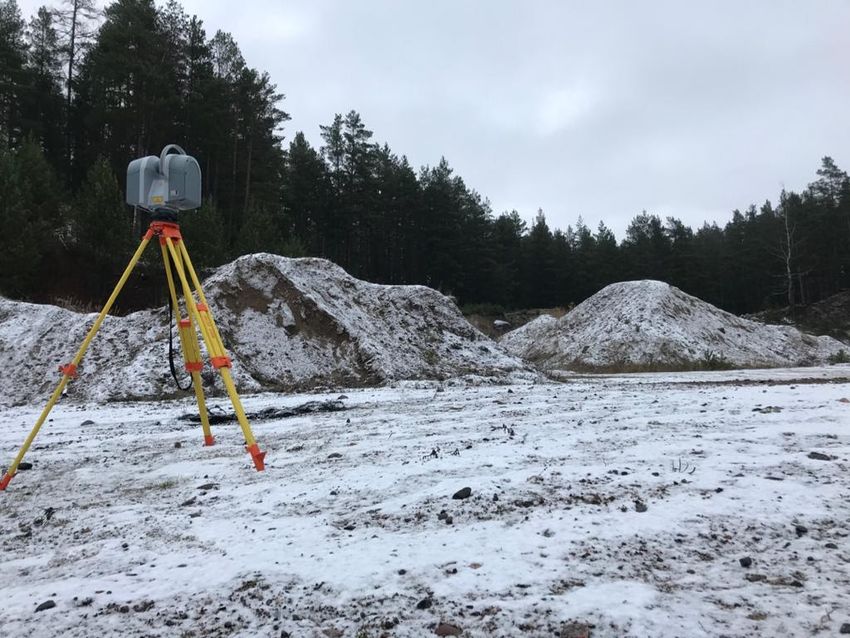

Abstract
In this thesis project, the main objective was to compare and evaluate three surveying methods
for volume determination: Photogrammetry, Terrestrial Laser Scanning (TLS) and Aerial Laser
Scanning (ALS) based on time consumption, efficiency and safety in the mining industry. In
addition, a volumetric computational method based on coordinates was formulated to estimate
the volume of stockpiles using lidar data captured with a laser scanner.
The use of GNSS receiver, UAV (Unmanned Aerial Vehicle) equipped with a LiDAR sensor as well
as a camera, and terrestrial laser scanner were adopted for making measurements on stockpiles.
Trimble Business Center and Trimble RealWorks were used in processing LiDAR data from TLS
and ALS. Two volume computational approaches were also explored using both TLS and ALS
LiDAR data. Agisoft Photoscan was used in processing the images captured adopting the structure
from motion principle. These softwares were used to estimate the volume of the stockpile. Matlab
was used to estimate the volume of stockpile using LiDAR data. A volume computational method
based on coordinates of point cloud was implemented in Matlab. Analysis based on time taken to
capture and process all data types till the final product was done. The results obtained from each
data capturing methods were evaluated. Simulated data technology is also adopted in this project
as it can be modeled in different ways to study the effect of surface roughness (point density) on
volume estimated. A part of this project explores the use of MATLAB to filter out unwanted
point clouds coming from the weeds that grow on the surface of an abandoned stockpile and also
surface areas that were to be excluded from the volume computation, as in this case.
From the results obtained, TLS and ALS do not differ much in the final volume estimates. Pho-
togrammetry on the other hand estimated a greater volume as compared to the other survey
methods. MATLAB in estimating the volume of stockpile achieves approximately an equal estim-
ate as that of the TLS and ALS within a short period of time. The point density and filtering
algorithm plays a critical role in volume computation which helps in providing a good estimate of
the stockpile. Findings from this project show that is it time consuming to estimate the volume
of stockpile using TLS and Photogrammetric approach. In terms of safety on an active mining
site, these two survey method have high risk probability as compared to the ALS approach. The
accuracy for the data captured and processed can be said to be satisfactory for each survey method.

Title Volume Calculation Based on LiDAR Data
Author AMAGLO Worlanyo Yao
Department Real Estate and Construction Management
TRITA number TRITA-ABE-MBT-21502
Supervisors Milan Horemuž and Krzysztof Gajdamowicz
Keywords Laser scanning, Volume, Stockpile, Photogrammetry, ALS, TLS,
. Mining, MATLAB, SfM

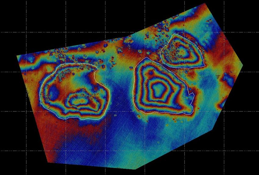
Sammanfattning
I detta avhandlingsprojekt var huvudmålet att jämföra och utvärdera tre kartläggningsmetoder
för volymbestämning: Fotogrammetri, Terrestrial Laser Scanning (TLS) och Aerial Laser Scan-
ning (ALS) baserat på tidsförbrukning, effektivitet och säkerhet i gruvindustrin. Dessutom for-
mulerades en volymetrisk beräkningsmetod baserad på koordinater för att uppskatta volymen av
lager med hjälp av lidardata som fångats med en laserskanner.
Användningen av GNSS-mottagare, UAV (obemannad flygbil) utrustad med en LiDAR-sensor
samt en kamera och markbunden laserscanner antogs för att göra mätningar på lager. Trimble
Business Center och Trimble RealWorks användes vid bearbetning av LiDAR-data från TLS och
ALS. Två volymberäkningsmetoder undersöktes också med både TLS- och ALS LiDAR-data.
Agisoft Photoscan användes vid bearbetning av de bilder som tagits och antagit strukturen från
rörelseprincipen. Denna programvara användes för att uppskatta volymen på lagret. Matlab
användes för att uppskatta volymen av lager med LiDAR-data. En volymberäkningsmetod baserad
på koordinater för punktmoln implementerades i Matlab. Analys baserad på den tid det tar att
fånga och bearbeta alla datatyper tills den slutliga produkten var klar. Resultaten från varje
datafångstmetod utvärderades. Simulerad datateknik antas också i detta projekt eftersom den kan
modelleras på olika sätt för att studera effekten av ytjämnhet (punkttäthet) på den uppskattade
volymen. En del av detta projekt utforskar användningen av MATLAB för att filtrera bort
oönskade punktmoln som kommer från ogräset som växer på ytan av ett övergivet lager och
även ytarealer som skulle uteslutas från volymberäkningen, som i detta fall.
Från de erhållna resultaten skiljer sig TLS och ALS inte mycket i de slutliga volymuppskattningarna.
Fotogrammetri å andra sidan uppskattade en högre volym jämfört med de andra undersöknings-
metoderna. MATLAB vid uppskattning av lagervolymen uppnår ungefär lika stor uppskattning
som TLS och ALS inom en kort tidsperiod. Punkttätheten och filtreringsalgoritmen spelar en
viktig roll i volymberäkning som hjälper till att ge en bra uppskattning av lagret. Resultat från
detta projekt visar att det är tidskrävande att uppskatta lagervolymen med TLS och fotogram-
metrisk metod. När det gäller säkerhet på en aktiv gruvplats har dessa två undersökningsmetoder
hög risk sannolikhet jämfört med ALS-metoden. Noggrannheten för de insamlade och bearbetade
uppgifterna kan sägas vara tillfredsställande för varje undersökningsmetod.

Titel Volymberäkning baserat på LiDAR data
Författare AMAGLO Worlanyo Yao
Institution Fastigheter och Byggande
TRITA nummer TRITA-ABE-MBT-21502
Handledare Milan Horemuž och Krzysztof Gajdamowicz
Nyckelord Laserskanning, Volym, Lager, Fotogrammetri, ALS, TLS,
. Brytning, MATLAB, SfM

Acknowledgements
First and foremost, I give glory, praise and thanks to God almighty for the gift of life and good
health thus has brought me thus far.
Secondly, I am deeply grateful to my academic supervisor Milan Horemuž for every form of support
provided during my studies and guiding me throughout my thesis. His prompt response to all
challenges solved via both zoom and physical meeting was really beneficial to the execution of my
thesis project. He took me up as more than just a student and I am grateful for that. I would
also like to thank my examiner, Huaan Fan for supporting my thesis project.
Thirdly, I would like to extend my sincere thanks to my external supervisor Krzysztof Gajdamowicz
for giving me this great opportunity to work in his renowned establishment, VISIMIND AB. He
makes limitless effort to make all the necessary provisions to obtain data required for my thesis
work, the comfort of working in his office and with his staff, and not forgetting the edibles that
come alongside working in the office. I would also like to thank Dawid Felczak for his assistance
in one of the crucial parts of my thesis work: Data Capturing. The hunt for a suitable study area
was hectic, yet a memorable and successful trip that was.
Finally, I must express my very profound gratitude to my parents, Dr. Joseph K. and Mrs. Rebecca
E. Amaglo and to my fiancée, Eugenia Y. Darko for providing me with unfailing support and
continuous encouragement throughout my years of study and through the process of researching
and writing this thesis. This accomplishment would not have been possible without them.
Special thanks to my close friends, Kwasi Nyarko Poku-Agyeman, Benedicta Osam-Pinanko and
Robert Antoh for their unconditional support throughout my studies in KTH Royal Institute of
Technology. Thank you.

iii

Table of Contents
List of Figures                                                                                             vi

List of Tables                                                                                             viii

1 Introduction                                                                                               1
     1.1   Motivation    . . . . . . . . . . . . . . . . . . . . . . . . . . . . . . . . . . . . . . . .     1
     1.2   Research objectives . . . . . . . . . . . . . . . . . . . . . . . . . . . . . . . . . . .         2
     1.3   Scope and Limitation      . . . . . . . . . . . . . . . . . . . . . . . . . . . . . . . . . .     2

2 Literature Review                                                                                          3
     2.1   Definitions . . . . . . . . . . . . . . . . . . . . . . . . . . . . . . . . . . . . . . . . .     4
     2.2   Total Station . . . . . . . . . . . . . . . . . . . . . . . . . . . . . . . . . . . . . . .       4
     2.3   GNSS receivers . . . . . . . . . . . . . . . . . . . . . . . . . . . . . . . . . . . . . .        5
     2.4   Unmanned Aerial Vehicles . . . . . . . . . . . . . . . . . . . . . . . . . . . . . . . .          6
     2.5   Laser Scanning . . . . . . . . . . . . . . . . . . . . . . . . . . . . . . . . . . . . . .        7
     2.6   Digital Elevation Model . . . . . . . . . . . . . . . . . . . . . . . . . . . . . . . . .         7

3 Methodology                                                                                                9
     3.1   Research Strategy . . . . . . . . . . . . . . . . . . . . . . . . . . . . . . . . . . . .         9
     3.2   Data Collection . . . . . . . . . . . . . . . . . . . . . . . . . . . . . . . . . . . . . .       9
           3.2.1   Case Study . . . . . . . . . . . . . . . . . . . . . . . . . . . . . . . . . . . .        9
     3.3   Data Processing     . . . . . . . . . . . . . . . . . . . . . . . . . . . . . . . . . . . . .    11
           3.3.1   GNSS-RTK Survey . . . . . . . . . . . . . . . . . . . . . . . . . . . . . . . .          11
           3.3.2   Photogrammetry (SfM) . . . . . . . . . . . . . . . . . . . . . . . . . . . . .           12
           3.3.3   Terrestrial Laser Scanning (TLS) . . . . . . . . . . . . . . . . . . . . . . . .         14
           3.3.4   Aerial Laser Scanning (ALS) . . . . . . . . . . . . . . . . . . . . . . . . . .          16
           3.3.5   Simulated Data (MATLAB) . . . . . . . . . . . . . . . . . . . . . . . . . . .            16
           3.3.6   LiDAR Data (MATLAB) . . . . . . . . . . . . . . . . . . . . . . . . . . . .              18

4 Analysis                                                                                                  19
     4.1   Volume Estimation . . . . . . . . . . . . . . . . . . . . . . . . . . . . . . . . . . . .        19
     4.2   Point Density . . . . . . . . . . . . . . . . . . . . . . . . . . . . . . . . . . . . . . .      19
     4.3   Noise . . . . . . . . . . . . . . . . . . . . . . . . . . . . . . . . . . . . . . . . . . . .    20

5 Results and Discussion                                                                                    21

iv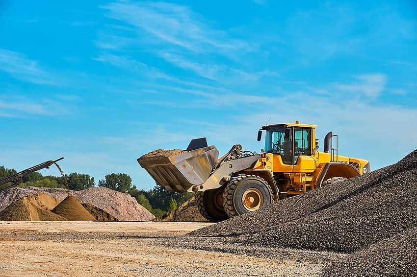

6 Conclusion and Recommendations                                                                   23

Bibliography                                                                                       24

Appendix                                                                                           26

A Appendix A                                                                                       26
  A.1 Photogrammetry . . . . . . . . . . . . . . . . . . . . . . . . . . . . . . . . . . . . .     26
  A.2 Terrestrial Laser Scanning . . . . . . . . . . . . . . . . . . . . . . . . . . . . . . . .   29
  A.3 Airborne Laser Scanning . . . . . . . . . . . . . . . . . . . . . . . . . . . . . . . . .    30
  A.4 MATLAB . . . . . . . . . . . . . . . . . . . . . . . . . . . . . . . . . . . . . . . . .     32

                                                                                                    v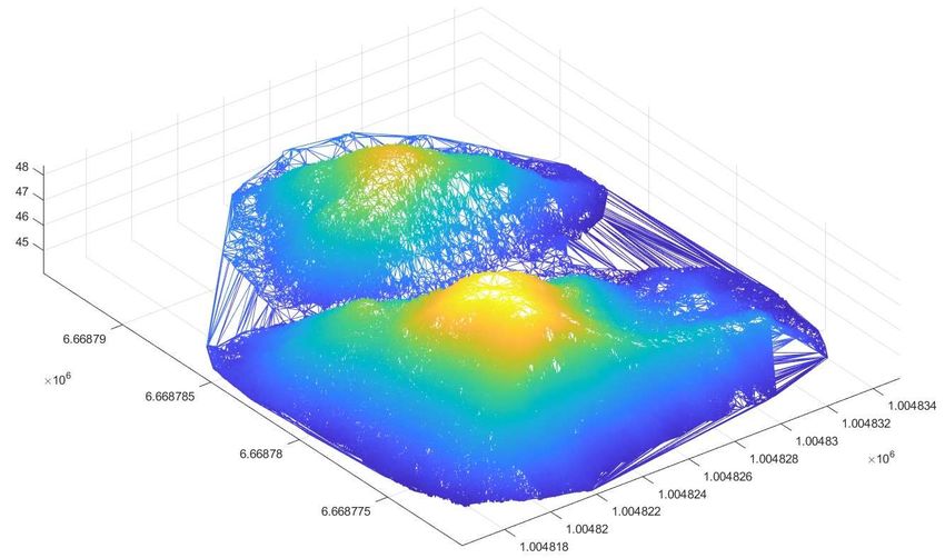

List of Figures
     1.1   Excavation on Mining site. . . . . . . . . . . . . . . . . . . . . . . . . . . . . . . . .       1

     2.1   Measuring with Total Station. . . . . . . . . . . . . . . . . . . . . . . . . . . . . . .        5
     2.2   Concept of RTK GNSS. . . . . . . . . . . . . . . . . . . . . . . . . . . . . . . . . .           6
     2.3   DSM and DTM. . . . . . . . . . . . . . . . . . . . . . . . . . . . . . . . . . . . . .           8
     2.4   Triangulated Irregular Network. . . . . . . . . . . . . . . . . . . . . . . . . . . . . .        8

     3.1   Aerial image of study area. . . . . . . . . . . . . . . . . . . . . . . . . . . . . . . .       10
     3.2   Measuring with Trimble TX8. . . . . . . . . . . . . . . . . . . . . . . . . . . . . . .         10
     3.3   Measuring with hexacopter UAV equipped with 6 intelligent flight batteries. . . . .             11
     3.4   Flowchart of data processing of SfM, TLS and ALS data. . . . . . . . . . . . . . .              11
     3.5   Measuring location of targets with RTK GNSS . . . . . . . . . . . . . . . . . . . .             12
     3.6   Step 1 to 4 . . . . . . . . . . . . . . . . . . . . . . . . . . . . . . . . . . . . . . . .     13
     3.7   Step 5 to 7 . . . . . . . . . . . . . . . . . . . . . . . . . . . . . . . . . . . . . . . .     13
     3.8   TLS scanning parameters. . . . . . . . . . . . . . . . . . . . . . . . . . . . . . . . .        14
     3.9   Six TLS stations . . . . . . . . . . . . . . . . . . . . . . . . . . . . . . . . . . . . .      15
     3.10 Accuracy of TLS station registration. . . . . . . . . . . . . . . . . . . . . . . . . . .        15
     3.11 Georeferencing errors . . . . . . . . . . . . . . . . . . . . . . . . . . . . . . . . . . .      15
     3.12 Simulated cuboid.      . . . . . . . . . . . . . . . . . . . . . . . . . . . . . . . . . . . .   16
     3.13 Simulated cuboid with surface roughness. . . . . . . . . . . . . . . . . . . . . . . .           17
     3.14 Indexed triangle. . . . . . . . . . . . . . . . . . . . . . . . . . . . . . . . . . . . . .      17
     3.15 LiDAR data in MATLAB . . . . . . . . . . . . . . . . . . . . . . . . . . . . . . . .             18

     4.1   Point Density in relation to volume estimation. . . . . . . . . . . . . . . . . . . . .         19

     5.1   Estimated Volume of Stockpile using LiDAR data            . . . . . . . . . . . . . . . . . .   22

     A.1 SfM Report . . . . . . . . . . . . . . . . . . . . . . . . . . . . . . . . . . . . . . . .        26
     A.2 Targets control accuracy. . . . . . . . . . . . . . . . . . . . . . . . . . . . . . . . . .       27
     A.3 Target controls error. . . . . . . . . . . . . . . . . . . . . . . . . . . . . . . . . . . .      27
     A.4 Image overlaps. . . . . . . . . . . . . . . . . . . . . . . . . . . . . . . . . . . . . . .       27
     A.5 Positional accuracy of targets. . . . . . . . . . . . . . . . . . . . . . . . . . . . . . .       28
     A.6 Boundary of stockpile use in Volume estimate. . . . . . . . . . . . . . . . . . . . .             28
     A.7 TLS overlaps. . . . . . . . . . . . . . . . . . . . . . . . . . . . . . . . . . . . . . . .       29
     A.8 DEM obtained from RTK GNSS topology data. . . . . . . . . . . . . . . . . . . . .                 29

vi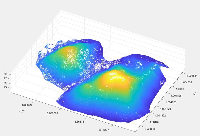

A.9 Stockpile surface model from TLS LiDAR data. . . . . . . . . . . . . . . . . . . . .          30
A.10 LiDAR data from ALS. . . . . . . . . . . . . . . . . . . . . . . . . . . . . . . . . .       30
A.11 DEM generated using LiDAR data from ALS. . . . . . . . . . . . . . . . . . . . . .           31
A.12 Stockpile surface model from ALS LiDAR data.. . . . . . . . . . . . . . . . . . . .          31
A.13 Untrimmed Surface. . . . . . . . . . . . . . . . . . . . . . . . . . . . . . . . . . . .     32
A.14 Trimmed Surface. . . . . . . . . . . . . . . . . . . . . . . . . . . . . . . . . . . . . .   32

                                                                                                  vii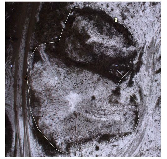

List of Tables
       3.1   Softwares used for estimating volume of stockpile based on data type. . . . . . . .         9

       4.1   Varying point density and corresponding estimated volume . . . . . . . . . . . . .         20

       5.1   Estimated volume of stockpile. . . . . . . . . . . . . . . . . . . . . . . . . . . . . .   21
       5.2   Summary of estimated volume from TLS and ALS LiDAR data. . . . . . . . . . .               21
       5.3   Summary of estimated time for Data capturing and processing. . . . . . . . . . . .         22

viii

1. Introduction
The mining industry is one of the leading communities in the west African sub-region which drives
the country’s economy. Most companies try to take advantage of the latest technology to improve
on their production and to maximise profit. As part of their operations, volume estimate update
is an essential part of the daily operations within the mining industry. The volume of stockpile
is important as the amount of crust excavated from an area need to be accounted for, relocating
stockpile requires the knowledge of the amount of crust being moved and also to keep records of
amount of crust accumulated for possible sales. With the aid of modern technology point cloud
and 3D models can be used to effectively estimate volume in a more efficient and precise way. In
this research I seek to use the point cloud and 3D surface model of a mass haul to estimate the
volume of stockpile in the mining field. This would make surveys of the mines safe for construction
workers as well as monitoring of mining progress for the construction manager.

Figure 1.1: Excavation on Mining site.

In the western part of Africa, Ghana to be precise, Gold mining is one of the top mineral mining
industries. Gold has a large market value, hence the high interest of most mineral mining compan-
ies. In gold mining, a large amount of earth crust is excavated to get access to gold hot-spots. In
doing so,the excavated crust is transported and offloaded at an assumed suitable space as shown
in Figure 1.1. The traditional method of estimating the volume of crust excavated i.e. ”before
and after” approach is unsafe,time consuming and inefficient to work in the mining industry. The
estimation of the existing volume of crust is a challenge as excavation work goes on by the hour.

1.1 Motivation
Laser scanning produces an output product known as point clouds, which represents surfaces of
various features on the earth. Such features consist of both natural and artificial objects. There
are natural minerals in the earth crust. Deep into the earth, deep drilling machines are being
used to extract minerals from the ground. These minerals are somewhat not easy to find. Mineral
mining industries go to great extents to obtain these rare minerals from the earth, hence large
volumes of earth crust being excavated. This project seeks to aid in maintaining the harmony
of a socio-ecological environment.There must be a balance in the extraction of minerals and the
natural habitat around us. In this project, focusing on the volume of crust excavated and offloaded,

point clouds from aerial photos and LIDAR scanners are used to calculate the large volumes of
crust offloaded at the assumed suitable space. The objective of this project is to assess the
survey methods for estimating volume of crust excavated (existing) using volumetric computation
with a number of software, which solves the issue of finding suitable zones for depositing such a
large amount of crust. This project was executed with supervision, assistance and resources from
VISIMIND AB, Stockholm, Sweden.

1.2 Research objectives
The main objective of this study is to evaluate three survey methods that yield the best results,
are efficient and the most convenient to be used in the mining industry. To be specific, the study
has the following objectives:
1. Evaluate survey method (UAV,TLS and ALS) based on area of site and timely result of data
captured and processed.
2. Evaluate the accuracy of volumetric estimation computed using Lidar data processing softwares
(Trimble Real Works and AGISOFT).
3. Simulate surfaces with variation in the surface properties (different roughness) for analysis
using volumetric computation methods in MATLAB.
4. To evaluate available data processing software on the market for volumetric computation of
point cloud data.

1.3 Scope and Limitation
The scope of this project covers three data capturing methods, the use of LiDAR data processing
software and the programming language, MATLAB, for computing volumes based on simulated
and actual LiDAR point clouds. The method for computation of volume is strictly based on the
coordinates of point clouds. Volume estimated in LiDAR data processing softwares would be
explored using the features and functions available in the software (i.e. EarthWorks in Trimble
Business Centre, TBC). However there are some limitations. In previous cases where large volumes
of stockpile existed, the volume could be computed from two generated surfaces (i.e. before-and-
after). In this case, there is no data on the surface before the stockpile was created hence this
project.

2. Literature Review
With the advancement in technology we have seen a great improvement of reconstructing reality
from precise point-wise measurement to represent an object to more continuous modeling of the
reality using 3D surface reconstruction. Global adaptation of the technology has grown over the
decade and hence much cost efficient, accurate and precise measurement of reality has vastly been
in different communities for various applications which include mining, construction and robotics.
In construction, the technology has made a major effect on how the construction industry pro-
gresses over a long period of time. The most recent progressions have benefited the industry in
endless ways. Extremely high costs are brought down, security rates are improved, and projects
are dealt with more proficiently. Moreover, the most recent technological devices and programs
permit administration groups to better keep track of projects and laborers remotely.
It is undeniable, innovation infringes on basically each perspective of or domestic and work lives,
which applies to customarily low-tech businesses such as construction. Fast progressions in tech-
nology, and the expanding rate of selection have driven to more secure and more effective work
destinations, decreased costs, quicker work completion and expanded profits. With the increasing
number of positive outcomes from high-profile, large-scale construction and framework projects,
indeed the techno skeptics of the industry are seeing emotional changes and are executing projects
in a collaborative and well organized environment.
In mining, specifically in the African sub-region, the mining industry in Sudan took a high interest
in exploration for fuel and minerals such as ore, iron, silver, chromite amongst others. The
products from the mines accounted for about 4% of gross domestic profit (GDP). With increasing
productivity over the years, Sudan has created a legitimate business for private companies to
invest in the mining sector (Khayal 2020). There has been similar growth in many other African
countries where the mining sector brought revenue to the country’s economy.
Several years ago, data capturing was more tedious to do. The use of chains, tapes, compasses,
electronic distance measuring equipment, theodolites, and total stations were what surveyors used
to map and make measurements of topographic features (Wolf 2002). These instruments are used
to measure distances, heights and angles of object positions. Measurements made with survey
equipment are represented using points which define the vertices or details of the object being
measured. These points are represented in x, y, and z coordinates. The equipment used in
capturing details of points have evolved over the years. Production of point clouds from data
captured can be developed directly or indirectly depending on the survey equipment used in
collecting the data. This has been studied by researchers in the field of geomatics and surveying
to assess the accuracy,efficiency and complexity of processing data into point clouds to produce
results. In categorizing point cloud development, images obtained from Structure from Motion
(SfM) are used to produce point clouds (Fonstad et al. 2013) which is an indirect process of
developing point clouds, whereas light detection and ranging (LiDAR) sensors produce directly
point clouds (Mancini et al. 2013). In recent times, LiDAR technology has proven efficient in
making measurements in almost every field of application,such as metal tracing in mining (Witt
2016), 3d mapping earthwork survey (Siebert & Teizer 2014), as-built BIM (Tang et al. 2010)
and many others. Some projects require collecting data from the field at given time demand.
There is the need for data to be captured over a period of time like in monitoring of construction
works (Pradhananga & Teizer 2013) where future decisions can be made in order to complete any
project earlier or in time. Point clouds basically depict the surface nature of the object scanned.
In other words digital surfaces are formed using point clouds as researched by Pluta & Domej
(2021). The surfaces are connecting polygons formed from a network of point clouds or can be
technically referred to as reconstruction of surface from point cloud scan as explored by Pluta &
Domej (2021), Erler et al. (2020) and Wang (2021).
There are various approaches to generating 3D models. The objective of most researchers is to
improve on existing algorithms to improve on them. This has brought about various methods of
constructing 3D models from point clouds. There are many application fields that require the need

for 3D models to be formed such as structural and mechanical components like pipes (Perez-Perez
et al. 2018), representation of features under water (Sarakinou et al. 2016), indoor navigation
(Dı́az Vilariño et al. 2016), mine roadway (Guo et al. 2016), train rails (Diaz-Benito 2012), etc.
Some techniques used in generating 3D models are cylinder projection method (Dı́az Vilariño
et al. 2016), Poisson equation reconstruction (Dı́az Vilariño et al. 2016), Delaunay triangulation,
amongst others. There are various survey instruments that can be used to collect point cloud
data for measuring the volume of the stockpile. In recent times, the most common instruments
used for earthworks are the total station, GNSS receivers, Unmanned Aerial Vehicle (UAVs)
and Laser scanners. These are all electronic measurement systems used in monitoring ongoing
projects on site. Total stations, GNSS receivers, cameras and laser scanners are capable of making
distance measurements of objects. These survey instruments have limitations based on the field
of application in which it is used.

2.1 Definitions
LiDAR is an acronym for Light Detection And Ranging. Laser scanning can be defined as the
use of a laser to collect dimensional data of objects in the form of a ”point cloud”. Point cloud is
a collection of points with 3D coordinates in a common reference system (Horemuz 2020). This
point cloud LiDAR data contains two types of information: metric and intensity.
Registration of point clouds is the transformation of all point clouds from different scan stations
to one station set up (home scan). Georeferencing is the transformation of point clouds to a
geographical reference system (external).
Photogrammetry in 3D is the process of extracting 3D information about objects in the environ-
ment from overlapping photographs and converting them from 2D to 3D digital models. Digital
Elevation Model (DEM) is one of many 3D data outputs of photogrammetry. Surface is the topo-
logy defined by point clouds from which volume measurements can be made. GNSS-RTK is one
of many modes of acquiring geographic positional coordinates using a Global Navigation Satellite
System device. “Real-time kinematic positioning is a satellite navigation technique used to en-
hance the precision of position data derived from satellite-based positioning systems such as GPS,
BeiDou, GLONASS, Galileo and NavIC” (Wikipedia contributors 2021).
Unmanned Aerial Vehicle (UAV) is an aircraft without a human on board. This device is mostly
controlled remotely. The system of a UAV comprises the following basic components for remote
operation, GPS, IMU, Camera and Antenna. These UAV devices are used for various applications
such as disaster study, shipping, wildlife monitoring, surveillance, photography, geographic map-
ping, engineering works. There are several kinds of UAVs in the market. The Matrice 600 is a
six-rotor flying platform designed for aerial photography and cinematography, as well as industrial
solutions. On board this system is a LiDAR system for scanning objects of interest.

2.2 Total Station
A comparative analysis was done with robotic total station and terrestrial laser scanner to es-
timate the volume of stockpile using different software (Pflipsen 2006). This search was done to
investigate the lowest number of point clouds to significantly change the volume estimated, also
time consumption and cost comparison was taken into consideration. The use of a total station
provides some level of accuracy to the estimated volume. Data collected using this method creates
fewer points as compared to point clouds from laser scanners or images from cameras and also the
depends on the distribution of measured points. This implies that when a total station is used, the
volume estimated from the measurement can be lower than that of the laser scanner or camera,
hence making estimates made from the total station less reliable. The density of points observed
is significant to attaining high accuracy measurements. The basic measurements the total station

takes are angles and distance which are used to obtain coordinates of points measured. There have
been technological advancements over the years, where a total station is being coupled with GNSS
receivers to acquire global referenced locations of objects. That principle of application is common
to all total stations. Totals station is mostly used for measuring regular surface objects like house
plan, road layout, boundary of water bodies, railway tracks, bridges, or setting out points in a
plane field for construction purposes, see Figure 2.1. Taking measurement of irregular surfaces for
volumetric estimation can be challenging as the surface of the object can not be entirely measured
hence some amount of volume would not be accounted for. It would be best to have the complete
surface of the object measured for best volume estimation.

Figure 2.1: Measuring with Total Station.

2.3 GNSS receivers
Satellites orbiting in space communicate with GNSS receivers on land. The Global Positioning
System (GPS) is used to track up to 31 satellites in space. These 31 satellites orbit the earth on
orbital planes with a number of satellites on each plane (Ershad & Ali 2020). GNSS is a position
location system that provides geographical positional information. This system consists of three
segments: user, control and space. Here, signal messages are transmitted on radio frequencies
common to each device. This mode of communication between satellites in space and positional
devices (GPS) has developed over the years. From static mode of acquiring a single position
over a long period of time, to RTK mode providing centimeter level accuracy in seconds with
fixed solutions. Thus, with the help of a reference base station, corrections can be transmitted to
increase positional accuracy. Static, Post processing kinematic and Real-Time Kinematic mode
are modes of observing GNSS data from satellites. It is also possible to post process data after
collection from the field. Studies have been made to explore and investigate the potential of using
GNSS receivers in the field of survey. Each mode has its advantages over one another and also
have their individual limitations on usage basis. The GPS aids in position location, navigation,
tracking and timing. GNSS was used in a similar project to capture the topology of the stockpile
and measure its volume. In the project the writer concludes that it is essential to have a high
density of points to achieve better results (Korall 2008).

Figure 2.2: Concept of RTK GNSS.

2.4 Unmanned Aerial Vehicles

Unmanned aerial vehicles (UAVs), or drones, are picking up in notoriety. These vehicles can be
controlled remotely or fly a preset way to perform studies based in locations of features and also
assess the progress of ongoing field projects. Improved models can take airborne video, pictures
and 3D pictures. UAVs are moreover supportive in checking logistics, performing site assessments
and surveying as-built works. Although numerous development experts may be concerned about
the costs and down to earth application of this modern innovation, the potential benefits and a
more long-term profit ought to exceed these concerns. UAVs are vehicles that are used in several
fields of application. They are mounted with different payloads depending on the purpose for
which it would be used. UAVs mounted with cameras have a lot of areas of application. They
can be used for photography, videography, surveillance, and photogrammetric purposes. In the
field of engineering, location is of high importance hence some UAVs are equipped with GNSS
receivers. Other UAVs can also be equipped with LiDAR sensors, which are used for laser scanning
in engineering works like structure monitoring, construction progress monitoring, deformation
monitoring, stockpile measurement for mining sites. The use of UAVs has proved beneficial in
many engineering fields. This technology has been adopted by all engineers to make their work
more easy and efficient. This has been so due to the numerous research made by researchers to
discover the potential of the system. It is generally known that the level of accuracy expected of any
survey instrument is dependent on the project in which it is to be used. Engineering construction
works would require higher accuracy and precision than object feature measurements. UAVs are
used regardless of project as it is only a mobile system carrying for the payload mounted on it.
A study was made using a DJI mavic air UAV as a photogrammetric approach to investigate
the applicability of UAV Photogrammetry for the estimation of the volume of stockpiles (Ajayi
& Ajulo 2021). In this project the researcher made comparative analysis with total station and
UAV based on processing time and accuracy. The data captured with the UAV was processed
using Agisoft Metashape Pro; this software was used to produce a digital elevation model which is
then used in estimating the volume of the stockpile. Data from the total station was processed in
ArcGIS to generate a triangulated irregular network (TIN) model from which the volume of the
stockpile can be estimated. A standard volume of the stockpile was obtained from a mill-machine
and used as reference measurement to the other two volume estimation methods. This paper also
concludes on UAV being accurate and time economical as well.

2.5 Laser Scanning
Laser scanning is defined as the process of using a laser to collect dimension data of objects in the
form of a “point cloud”. These point clouds are used to define the shape of objects in a process
known as reconstruction or modeling (Horemuz 2020). Instruments with laser sensors for scanning
are laser scanners. There are two types of sensors, active and passive. Passive sensors detect the
reflected or emitted electro-magnetic radiation from natural sources, while active sensors detect
reflected responses from objects which are irradiated from artificially generated energy sources,
such as light radar. The laser scanner has the advantage of obtaining centimeter level precision.
This makes reconstructing the scanned object highly detailed and close to the actual object. This
technology is used in most archaeological works where ancient buildings are scanned and modeled
in 3D for analysis and making future improvements to it. High density point clouds can be
obtained from the terrestrial laser scanner, which improves the ability of the modeled point cloud
to fit the real surface of the object. Reverse reconstruction of features with point cloud is a method
of modeling real features into a digital format. TLS scanner is the most robust scanning system
and takes technical know-how to capture data efficiently.
In a study (Pflipsen 2006), a terrestrial laser scanner and total station was used in surveying
stockpiles in a project. In this project a number of targets are placed on and around the stockpile.
The laser scanner was used to scan the stockpile as well as the target. The TLS scanner was
mounted at different positions to be able to scan the entire surface of the stockpile. The researcher
used data processing software, Cyclone, Geo and Geograf to process the field data. Comparison
between Cyclone and Geograf based on reduction of the number of point clouds. At the end of
the project it was concluded that the number of points affects both the time taken to capture the
data as well as processing it. The researcher went further to advise that it would not be advisable
to purchase a laser scanner for just volumetric estimation projects. Should a laser scanner be
available where the time to execute the project is short, it is best to use that for data capturing
and also have control over the number of point clouds used for processing (Pflipsen 2006).

2.6 Digital Elevation Model
Digital Elevation Model (DEM) is the representation of the surface of the earth without objects
or features. Digital Surface Model (DSM) is the representation of the surface of all features on the
earth. Digital Terrain Model (DTM) is the representation of the terrain of the ground including
the natural terrains of water bodies which can be generated from points from a number of survey
instruments. The data collected is required to be dense enough to depict the nature of the surface
of the ground. The height measurements obtained from DEM is used as the reference height from
which volumetric measurements are made. There are a number of methods for which the model
could be formed.
Triangulated Irregular Network (TIN) is one of many methods that is used to model a surface.
This method uses a network of triangles with varying sizes to create a surface model using the
point clouds. The set of vertices used in constructing the network in this case are the point clouds
which are connected with each other with an edge to form a network of triangles.

Figure 2.3: DSM and DTM.

    Figure 2.4: Triangulated Irregular Network.

8

3. Methodology
3.1 Research Strategy
Volumetric estimation from point cloud data sets are estimated using different volumetric compu-
tational methods. The goal of this study is to identify optimum surveying and processing methods
for volume determination. The use of different survey methods to capture the same sample data
contributes to the results obtained after processing. Each of the methods of survey have their
independent limits and setbacks to the accuracy of measurement taken. With simulated data, a
regular shape of 3D point cloud is created and the volume computed based on coordinates. Given
this simulated data, variation in surface roughness would be introduced as noise and the effect of
noise and point density on the result of volume estimated would be assessed.
Three survey methods are implemented in capturing field data of two different study cases. With
the help of a GNSS-RTK device and targets or markers as ground control points are surveyed
and used in georeferencing the lidar data during processing. Geographic information data can be
managed and improved using software capable of processing spatial data. Software that have the
capability to process Lidar data is used for this study.
Data collected would be thoroughly examined and cleared of all noise so as to generate precise di-
gital elevation models (DEM) and achieve accurate measurements. For the data (images) obtained
from UAV, Agisoft photoscan is used in processing the images. Lidar data obtained from TLS
and ALS is processed using Trimble Real Works (TRW). A list of software capable of estimating
the volume of the stockpile is provided amongst which one software is tested. One actual study
area and one simulated data would be considered for this analysis. Software for computing the
volume of data is shown in Table 3.1.
UAV TLS ALS
S1 AGISOFT TRW TRW
S2 - MATLAB MATLAB
Table 3.1: Softwares used for estimating volume of stockpile based on data type.

S1 (actual) and S2 (simulated) are the data under study used to determine and compare the
volumetric computational methods of the data. Find the difference in measurement of both study
areas to determine a suitable volumetric computation method that best fits the nature of the
surface to the crust. A theoretical approach to computing the estimated volume of material using
point cloud data obtained from lidar sensors and coordinates of simulated data was implemented
using MATLAB.

3.2 Data Collection
3.2.1 Case Study
For S1 field (actual) data, a suitable site was located in Trosa, the south-western part of Stockholm.
In this study area was an abandoned quarrying site with stockpiles. These stockpiles were partially
covered in snow at the time of the survey as shown in Figure 3.2 .All three data capturing methods
were used to survey the stockpiles.
Trimble TX8 is one of Trimbles 3D laser scanners. It is able to make a 360° scan with its vertical
rotating mirror on a horizontal rotating base as shown in the Figure 3.2. It has the capability of
scanning 1million points per second, with a standard scanning range of 120 meters which can be
extended to 340 meters.
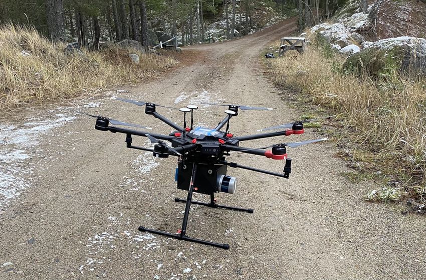
The ALS is a custom designed aerial scanning system suitable for UAVs and easy to operate. This
is a customized Matrice 600 Pro, a hexacopter UAV equipped with 6 intelligent flight batteries
that extends the flight time of the UAV for a longer duration. Onboard this hexacopter is an IMU
capable of being integrated with an RTK GNSS receiver to obtain centimeter level positioning.

Figure 3.1: Aerial image of study area.

                           Figure 3.2: Measuring with Trimble TX8.

It also comes with an ortho camera, Manta G-1236, a 12.4MP machine vision camera as shown in
the Figure 3.3. A laser scanner was integrated into the system to obtain LiDAR data. Velodyne
Ultra Puck is a 360° horizontal scanner with a 40° vertical field of view which produces high-density
and long-range intensity data. The Ultra Puck tops it class when it comes to intensity calibration
and accuracy.

10

Figure 3.3: Measuring with hexacopter UAV equipped with 6 intelligent flight batteries.

3.3     Data Processing
Shown in Figure 3.4 below is a flowchart of how images from SfM and LiDAR data from TLS and
ALS are processed before finally estimating the volume of stockpile.

             Figure 3.4: Flowchart of data processing of SfM, TLS and ALS data.

3.3.1    GNSS-RTK Survey
This mode of position acquisition was used to pick the topographic nature of the earth surface.
The topographic nature of the ground was needed to visualize the flatness of the area where the
stockpiles are located. This data was used to generate a digital terrain model which was also used
as a reference surface for the stockpile. The positions of black and white targets distributed as
well as the instrument station of the terrestrial laser scanner were surveyed also. This data was
used in the georeferencing stage of point cloud processing. Digital elevation model was generated

                                                                                               11

with the spot height data collected on site. This DEM was generated in TBC using the surface
creation tool. This surface was used as the before surface and a reference height from which the
volume of the stockpile was computed.

Figure 3.5: Measuring location of targets with RTK GNSS

3.3.2 Photogrammetry (SfM)

Structure from Motion (SfM) principle was adopted to generate the point clouds for volume
estimation and generating an orthophoto map. For images captured, markers were reasonably
distributed within the study area and surveyed for point cloud registration and georeferencing.
Having captured images of the site simultaneously with the ALS, 113 images were processed in a
photogrammetric software called Agisoft Photoscan. The images imported were initially aligned
with the help of tie points to get the camera position and orientation for each of the images as
captured, see step 1 in Figure 3.6. The default alignment parameters are used to produce sparse
point clouds.
Next, the GPS data containing the locations of the 10 targets or markers placed on the ground
were imported and identified in the all 113 images. This is done to aid the system automatically
find the images that have similar targets in them. The higher the number of images used to
identify a target, the closer the estimated position of the target automatically identified in the
images. In doing so the images are transformed into the desired external coordinate system, in
this case SWEREFF99 TM, see step 2 in Figure 3.6.
Reconstruction of dense point clouds are generated to develop a 3D model of the stockpile as
shown in step 3 and 4 in Figure 3.6 . With high density point cloud, meshes can be created to
visualise the stockpile as shown in step 5 in Figure 3.7. From the dense point cloud and mesh, a
DEM is generated as well as an orthophoto, see step 6 and 7 in Figure 3.7.
A volume estimation tool is available in Agisoft Photoscan. The algorithm for calculating the
volume from point clouds is based on the surface difference where the algorithm defines a reference
or base surface based on a user-defined boundary enclosing the area for which the volume is to be
measured.

Step 1                             Step 2

Step 3                             Step 4
         Figure 3.6: Step 1 to 4

Step 5                             Step 6

                  Step 7
         Figure 3.7: Step 5 to 7

                                            13

3.3.3 Terrestrial Laser Scanning (TLS)

The laser scanner is leveled and a preview scan is made from which the objects of interest to be
scanned are being selected in the preview. Scan settings were configured as shown in the Figure
3.8
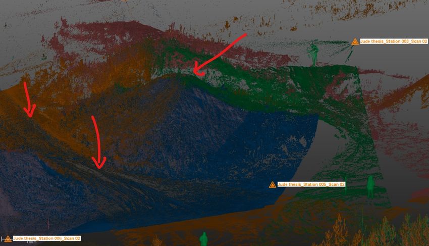
This is the scanning configuration used for all 6 scan stations with an approximate scanning time
of about 20 minutes per station, see Figure 3.9 . The time taken for the TLS to scan the stockpile
completely was about one hour and 45 minutes including time to move to a new station and re-level
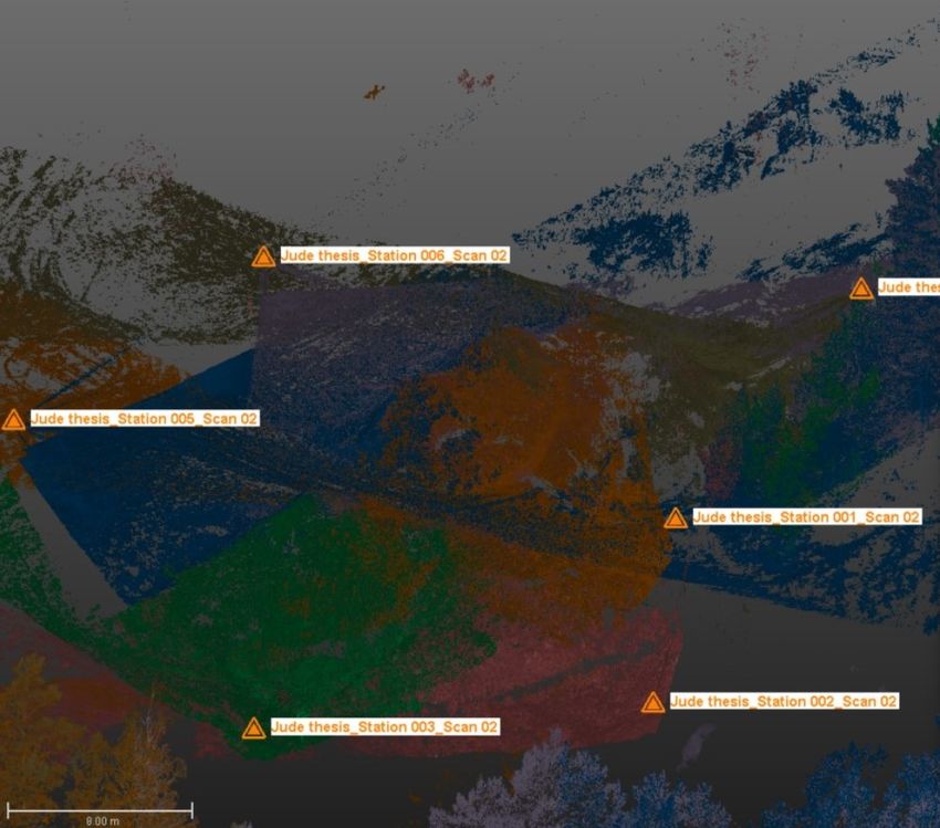
the scanner. In order to completely scan the stockpile, six scan stations were established. The
position of these scan stations were surveyed with the GNSS-RTK instrument. The job files were
exported into Trimble realworks where cloud to cloud manual registration was done, see Figure
A.7. This registration was done with one scan station set as the home scan. Point clouds were
registered in pairs until all scans were registered into one coordinate system and the errors were
acceptable as shown in Figure 3.10. The overall Cloud to Cloud error was 6.51 mm with maximum
error of 18 mm between scan station 001 and 002, and minimum error of 3 mm between scan
station 005 and 006.
Georeferencing of the registered point cloud was done by assigning the geographical coordinates
obtained from the GNSS-RTK data collected on the field. The six coordinates of the TLS in-
strument setup stations were observed with fixed solutions which guarantee a high accuracy of
the stations location. The instrument height was inferred from the difference in the height of the
point cloud closest to the setup station and the height obtained from the GNSS-RTK device. The
average error margin after georeferencing was quite reasonable as the height factor plays a role in
the transformation and rotation matrix of the point cloud, results as shown in Figure 3.11.
In Trimble Business Center (TBC), clearing point clouds of all noise was done both manually
and automatically. The automatic process of clearing unwanted points from point clouds involved
ground classification. This function was executed at the click of a button applied to the selected
point cloud input. With the new set of classified point clouds a boundary was defined using a
polyline vector layer to enclose the area where the measurement was made. Using the surface
creation tool, a surface layer was generated for the set of unclassified point clouds in order to be
used in the volume estimation tool, see Figure A.9.

Figure 3.8: TLS scanning parameters.

Figure 3.9: Six TLS stations

  Figure 3.10: Accuracy of TLS station registration.

Part 1                                           Part 2
         Figure 3.11: Georeferencing errors

                                                          15

3.3.4    Aerial Laser Scanning (ALS)
Data capturing with the ALS took about 45 minutes to scan an area of about 12, 300 m2 . Data
from ALS was processed with a private software called Data Processing Module (DPM). The point
clouds were processed in the same steps as data from TLS with final processed data as shown in
Figure A.10. Similar visual output of stockpile mesh and DEM from ALS data was generated as
shown in Figure A.12 and Figure A.11 respectively.

3.3.5    Simulated Data (MATLAB)
In the initial stages of using MATLAB to estimate volume of an object, regular shaped 3D figures
were used to test the initial volumetric computation. 3D points representing the vertices of a
cuboid were generated, see Figure 3.12. The approach to computing the volume is based on the
use of the coordinates of the vertices. The product of the difference between the maximum and
minimum value of each axis, i.e dimensions of cuboid, gives the volume of the cuboid. This was
quite a straightforward approach to computing the volume for a regular 3D shape. Having created
a 3D cuboid with dimensions 2 m x 5 m x 10 m, a computed volume of 100 m3 is obtained.
Next, a number of random 3D points with varying heights were generated to the top surface of
the cuboid to depict roughness on the surface as shown in Figure 3.13. This variation was based
on the density of points. In doing so, the initial computation method for calculating the volume
of the new cuboid would be inaccurate hence the need for a different computational method.

                                Figure 3.12: Simulated cuboid.

From Figure 3.14, A, B and C are the vertices of a triangle that forms part of the mesh surface
of the stockpile. The area is computed from the coordinates and multiplied by the difference in
height of the 3 vertices from the reference height. Delaunay function was implemented to generate
indices for a triangulated irregular network of 3D points. A geometric mathematical approach for

16

Figure 3.13: Simulated cuboid with surface roughness.

                                  Figure 3.14: Indexed triangle.

computing the volume of objects with irregular surfaces based on the coordinates was implemented.
The formula adopted for this computation is as shown in the equation 3.1 , (John D 2011).

                      h                                   i
                          Ax(By−Cy)+Bx(Cy−Ay)+Cx(Ay−By)
                                                                   Az+Bz+Cz               
          V olume =                     2
                                                              ×        3       − Ref.Height    (3.1)

A study was done using this simulated data to make inference on the effect of noise and point
density on the volume estimated.

                                                                                                 17

3.3.6    LiDAR Data (MATLAB)
A crucial part of undertaking this project is studied in this section. The possibility to estimate
the volume of stockpile using data collected from TLS or ALS without reference surface data is
explored. Thus, capturing data using a laser scanner and importing the point clouds directly in
MATLAB for volume estimation. It is of essence that the LiDAR data is prepared before being
imported to MATLAB. LiDAR data has to be registered, georeferenced, if needed, and trimmed to
the area of interest before exporting to .txt format. The only parameters required and necessary
for computing the volume of the stockpile in MATLAB are the three coordinates of the point
cloud (x, y and z coordinates). The algorithm implemented for volume computation of simulated
data is applied here on actual LiDAR data. LiDAR data imported in MATLAB is visualized as
seen in the Figure 3.15.

                            Figure 3.15: LiDAR data in MATLAB

In cases where there is a small amount of noise, for example weeds on the surface of stockpile,
a filter function is implemented to exclude such noise from being added to the total estimated
volume

18

4. Analysis
4.1 Volume Estimation
In estimating the volume of the stockpile from LiDAR data, two approaches were used. approach 1,
volume estimate based on stockpile surface and stockpile boundary whereas approach 2 calculates
the volume based on stockpile surface and surface of ground (DEM). In Approach 1, the selected
surface is set as the final surface and the initial surface is defined from the stockpile boundary.
Where the surface is above the boundary, cut is computed (stockpile); where the surface falls below
the boundary, fill is computed (depression). In Approach 2, the Initial surface is the original surface
and Final surface is the stockpile or surface after excavation. Where the Initial surface is above
the Final surface, then cut is computed; where the Initial surface is below the Final surface, then
fill is computed.Volumes are computed only in areas where the initial and final surfaces overlap.
The advantage of Approach 1 is that a the precise area of stockpile for measurement is well-
defined. Approach 2 has the advantage of considering the slanted surface within the overlapping
region. However, Approach 2 is most likely to underestimated that area of stockpile in the volume
estimation as some regions within the boundary would be below the actual reference surface of
the ground.

4.2 Point Density
The number of points is a major factor in estimating the volume of stockpile. Points obtained
from any scan system helps define the geometry of the stockpile. It can be said that, more points
obtained by the scanner increases how detailed the scanned object is. A well defined object gives
high precision and accuracy in measurements made. For this reason, 100, 500, 1000, 5000 sets of
random points were simulated to observe the precise volume as compared to the actual volume of
the cuboid. Based on the results in Table 4.1, conclusions can be made.
From the graph shown in the Figure 4.1, it is noticed that the point density influence the estimated
volume in m3 which increases but never attains the absolute volume of 100 m3 . From this we can
interpolate the estimated volume from a specific number of random points and vice versa.

Figure 4.1: Point Density in relation to volume estimation.

Table 4.1: Varying point density and corresponding estimated volume
              Number of random points                Estimated Volumes(m3 )
                         100                                  94.19
                         500                                  95.90
                         1000                                 96.75
                         5000                                 97.30

4.3     Noise
LiDAR data would normally have noise in the data. In the LiDAR data captured, weeds growing
in the surface of the stockpile were picked up by the laser pulse and interfered as object in the
data. This point cloud noise forms part of the data hence reducing the precision of volume to
be estimated. Filtering out these noise point clouds is necessary to get the right volume when
making measurements. Due to the vertical nature of weeds growing on the surface of the stockpile
a vertical pattern is observered which inturn creates a longer distance as compared to the distance
pattern between the point cloud of the stockpile when the TIN function is applied. This noise
point cloud can be filtered out or trimmed out by observing the trend in the length of the sides of
the triangles. The difference in results before and after filter can be seen in Figure A.13 and A.14
under the appendix section.

20

5. Results and Discussion
The topology of the site surveyed with the RTK GNSS receiver was close to a plane surface with
maximum and minimum height of 47.2 m and 44.6 m. With a height difference of about 2.6 m,
it can be said that the surface around the stockpile is relatively flat, see Figure A.8. This is the
surface assumed to be the initial surface before the stockpile existed. The DEM generated from
this surface shows a peak height at the north-eastern region of the DEM.
Reports from initial image processing is as shown in Figure A.1. The ten markers were identified
during image registration and their positional error and accuracy of control points after registration
is as displayed in Figure A.2, Figure A.3 and Figure A.5. The positional accuracy is within a
margin error of ±1.8 cm of which one target, m29a, being an outlier with value −3 cm. This could
be as a result of misidentifying the central position of the target in the 7 images it was identified
in. The total error obtained after registration was 20 cm. The registration result is acceptable for
this study. It can also be seen in the Figure A.4 that the minimum number of images overlapping
is 1 and over 9 images had an overlap. This shows that the data captured is good and has no
gaps; in other words, all areas of the stockpile and its neighboring areas were captured. The area
of scan is 0.01662 km2 of which 3% is the area of the stockpile being measured, see Figure A.6.
The estimated volume of stockpile measure in the Agisoft photoscan is 363.43 m3 as shown in the
volume report generated, see Table 5.1.

Table 5.1: Estimated volume of stockpile.
Perimeter Area (m2 ) Volume Volume Volume
(m) above (m3 ) below (m3 ) total (m3 )
Stockpile 75.600 357.706 363.437 8.128 355.309

The TLS produced over 50 million point clouds of which not more than 3.3% of the point clouds
were under study. The overall cloud to cloud error obtained after registration was of maximum,
17.89 mm and minimum, 3.22 mm, see in Figure 3.10. The point clouds were georeferenced as
well. From the mesh created, the maximum and minimum height of the stockpile was 49.9 m
and 44.7 m respectively. With a boundary of area 325 m2 , the volume of stockpile within the
boundary was measured with the results displayed in Table 5.2.

Table 5.2: Summary of estimated volume from TLS and ALS LiDAR data.
SURVEY METHOD APPROACH A (m3 ) APPROACH B (m3 )
TLS 361.2 372.3
ALS 359.2 375.6

Data obtained from ALS was already processed. The same boundary used in estimating the
volume of stockpile from the TLS data was applied. The reason for this is to be able to estimate
the volume of the same area of stockpile and compare the results. From the results we can see
that the estimated volume is definitely affected by the mode of capture, slight variation in the area
of stockpile defined by the boundary used, as well as the methodological approach of computing
the volume. An overall difference of about 2 − 3 m3 irrespective of the mode of data capture or
approach is not so significant for this analysis.
In MATLAB, the algorithm for filtering noise and computing the volume of stockpiles based on
coordinates is one of the research objectives. The fundamental volume equation would only hold
for a regular shaped object. In the case of the 3D cuboid with dimensions 2 m x 5 m x 10 m, a
computed volume of 100 m3 is obtained. Hence the test to determine the effect of surface roughness
on the volume estimated was possible by varying the number of points that form the surface of
the figure. An increase in the number of points forming the surface gets the estimated volume
closer to its absolute volume. Adopting the Delaunay function immensely eases the computation
of volume. It allows the user to calculate the area based on each triangle that forms the surface
mesh of the stockpile. Being able to do this, the height factor becomes an essential part of the
computation. The height of each vertex of a triangle is the difference between the reference height

and the height at the surface. With a reference height of 44.5 m, an estimated volume of 375.29 m3
was achieved immediately after hitting the RUN button as shown in Figure 5.1.

Figure 5.1: Estimated Volume of Stockpile using LiDAR data

The time taken for each survey method is estimated and recorded for analysis as shown in Table
5.3. From the tabulated result, it can be observed that TLS take much longer time as compared
to the other two data capturing methods. This is because of the number of scan stations required
to scan the stockpile from all angles. In the processing stage, SfM has the maximum processing
time due to the number of images as well as the level of processing required. ALS has a lower
processing time as it does not require cloud-to-cloud registration of scenes, that is point clouds
from ALS are in the same orientation. MATLAB has the least processing time. Amongst the
three survey methods, ALS has the least time duration for capturing, processing, and estimating
the volume of stockpile.

Table 5.3: Summary of estimated time for Data capturing and processing.
SURVEY CAPTURING PROCESSING TOTAL (hr)
METHOD (hr) (hr)
SfM 0.5 4-5 4.6-5.6
TLS 1.7 2-3 3.7-4.7
ALS 0.6 1.5 2.1
MATLAB - 0.2 0.2

6. Conclusion and Recommendations
Based on area of site and timely result of data captured and processed as shown in Figure 5.3, it
can be confirmed from the scope of this project that ALS is the most efficient survey mode for
capturing and processing data. Should there be the challenge of ALS not being available TLS is
recommended but for data processing, the best method is to extract coordinates from Lidar data
and then compute the volume separately using MATLAB or any other programming language.
The accuracy of volumetric estimation computed using Lidar data processing software varies. In
Agisoft, the user could barely have control over the data while processing. Right from processing
of images to generating orthomosaic the user can only choose from a limited list, other processing
parameters to be applied to the data. Like in the estimation of volume, that software required the
user to define the boundary for which the point clouds within the boundary would be included
in the volumetric computation. The software by default uses the best fitting plane to define the
reference surface of the stockpile. This computational workflow method is biased. In TRW/TBC,
the user has more control over the data as to the number of points to be used in processing,
reference surface data to be used in estimating the volume, etc. This improves the accuracy of
data used in estimating the volume of stockpile. Conclusions to be drawn from the result from
the analysis of simulated surfaces with variation in the surface roughness suggest that depending
on the volumetric computation method implemented in MATLAB, the algorithm would not be
flexible enough to take into consideration the surface roughness of the object. The user needs to
have full control of the point cloud to be included in the volume estimation, hence the need for
a more flexible volumetric computation method. Coupling of these functions breaks the barrier
between volume estimation of regular and irregular 3D shapes.
To determine the feasibility of a survey method to any given ground nature to produce the best
accuracy for analysis, accessibility of the site is important. ALS draws a huge gap between itself
and TLS when it comes to topology, accessibility and safety. Comparing the time factor and
estimated volume with both survey methods, ALS is suitable for both accessible and inaccessible
sites and very undulating topology. It is obviously safe for mining sites as the survey does not
need to be present on the field. ALS can be used to produce volume estimates as often as the
site manager wishes. SfM, is not recommended in any aspect of this project as it poses harm to
the surveyor on a mining site and takes so much time to capture and process data for a single
estimate.
From previous research works done in relation to this thesis, available data processing software
on the market for volumetric computation of point cloud data are Agisoft Photoscan, Geograf,
Cyclone, Trimble Business Center, ArcGIS, Global Mapper, Quantum GIS, and many more.
Overall, volumetric estimation based on coordinates of point clouds in MATLAB, is dynamic
and flexible for the user to manipulate the algorithm to suit the Lidar data captured. The user
only needs a well prepared LiDAR data before importing into MATLAB for the script to run
successfully.

You can also read