Vol. IV - Global climate change impacts on natural systems in the Lombardia region
←
→
Page content transcription
If your browser does not render page correctly, please read the page content below
Technical Summary                                                                                pag. 1

Vol. IV - Global climate change impacts on natural systems
in the Lombardia region
Unità Operativa: Politecnico di Milano

According to the IPCC Fourth Assessment Report, published in October 2007, “warming of the
climate system is unequivocal, as is now evident from observations of increases in global average
air and ocean temperatures, widespread melting of snow and ice and rising global average sea
level” (IPCC, 2007). Anthropogenic emissions of greenhouse gases are today identified with a very
high level of confidence as the cause of relevant impacts on natural systems; in the coming years
these emissions can sensibly impact human activities, such as agriculture, water supplies, human
health or ecosystems. Climate is in fact one of the factors that determines natural systems
composition, productivity and structure. A great number of plants can successfully grow and
reproduce only in a specific range of temperatures and precipitation regimes; at the same time,
meteo-climatic conditions affect fauna geographical distributions, together with food resources
availability. Climate change, thus, can affect ecosystems, populations and individuals directly (e.g.,
owing to the increase of average temperature) or indirectly (e.g., through changes in food resources
availability).
A comprehensive albeit qualitative assessment of climate change impacts is described in Volume II
of this report. The quantitative analysis of all the expected impacts on natural systems in Lombardia
is extremely complicated and is beyond the scope of this project. Therefore, in this volume we
present a study on climate change effects for few charismatic species that characterize the habitats
of the Lombardia region: the alpine ibex (Capra ibex ibex) in Parco dell’Adamello; the brown trout
(Salmo trutta) in the upper portion of river Adda; the black grouse (Tetrao tetrix tetrix) in the Parco
dell’Alpe Veglia-Devero; the chamois (Rupicapra rupicapra) in Valchiavenna. As climate change
impacts on vegetation are expected on long timescales, the attention is thereby directed toward
animal species, because of the shorter time scale of the response to climatic variation. Habitat
suitability models have been used to study climate change impacts; these models evaluate the
suitability of a certain area for a specific species on the basis of the area characteristics. Habitat
suitability models describe the relation existing between presence and abundance of a species and
habitat characteristics (morphological, climatic, vegetational, anthropic). Using these relations, it is
possible to estimate information such as suitable areas and potential number of individuals that can
be sustained by a defined area.
Finally, climate change impacts on the population dynamics of alpine ibex (Capra ibex ibex) have
been studied, focusing on the population in Parco del Gran Paradiso. In this analysis, scenarios of
climate change were regionalised to derive stochastic series of local daily precipitation and
temperature from trends simulated by global models.

Alpine ibex (Capra ibex ibex)
A first analysis was conducted on alpine ibex (Capra ibex ibex), a charismatic species, threatened
with extinction in the recent past, in Parco dell’Adamello (Figure 1). The Parco dell’Adamello
forms, together with the four adjacent parks (Figure 2), one of the biggest protected areas of Europe
(more than 250,000 ha). The 3,000 m of altimetric range between the lowest and the highest
altitudes (from 390 to 3,539 m above sea level) determines climatic changes which, with
lithological differences, affects structure, composition and distribution of the ecosystems in the
Parco. During the XVIII century, the alpine ibex was gone extinct because of intense hunting and

Progetto Kyoto Lombardia – Linea Esternalità Ambientali (2008)         Technical Summary - Terzo Anno
Technical Summary pag. 2
poaching. Between 1994 and 1997 and since 2000, re-introduction operations in the Parco
dell'Adamello were carried out; therefore it is important to know how ibex will respond to climate
change for re-stocking operations to be completely successful.
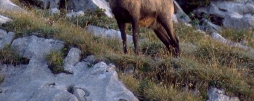
Figure 1: The ibex (Capra ibex ibex) in Parco dell’Adamello.
Figure 2: Adamello, Adamello-Brenta, Stelvio and Engadina parks.
The optimal habitat for alpine ibex is characterised by rock slopes facing south, beyond the tree
line, mixed with meadows and cliffsides up to the snow limit. In the summer, alpine ibex prefer
high altitudes, up to above 3,000 m; during winter, steep slopes, facing south, are preferred between
1,800 and 2,500 m, where snow slides down leaving the grounds uncovered. During winter and
spring, alpine ibex move downhill towards coniferous forests; in particular, in springtime they move
towards lower altitudes seeking for grass in the forest.
The habitat suitability of Adamello has been studied with model that consists of two submodels:
one for winter and one for summer habitat suitability (Pedrotti e Tosi, 1996; Ranci Ortigosa et al.,
2000). The wintering model depends, via discrete functions, on altitude, aspect, slope and
vegetation; function values are listed in Table 1. The habitat suitability function for the wintering
model is defined by the following expression:
Habitat Function = (Altitude + Slope + Aspect) * Vegetation.
Progetto Kyoto Lombardia – Linea Esternalità Ambientali (2008) Technical Summary - Terzo Anno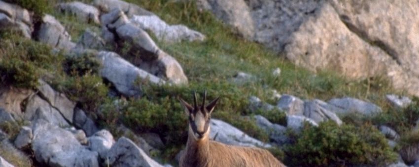
Technical Summary                                                                                                pag. 3

The winter habitat suitability function varies between 0 and 9. Suitability classes are four; each
class defines ibex potential density, as reported in Table 2.
The aestivation model depends on altitude only. The suitability function is equal to one (suitable
area) if altitude is higher than 2,000 m, and to zero (non suitable area) if it is lower. Ibex potential
density is defined in Table 2.

                  Table 1: Habitat suitability model: ibex wintering model (Pedrotti e Tosi, 1996).
                                                   Score                                        Score
            Environmental Variables               Winter          Environmental Variables       Winter
            Altitude                                              Aspect
            1200-1500                                 1           180-202 (W)                       1
            1500-1800                                 2           202-293 (SW-S)                    2
            1800-2200                                 3           293-337 (SE)                      3
            2200-2400                                 2           337-360 (E)                       1
            2400-2600                                 1           Slope
            Vegetation                                            30°-35°                           1
            Forest with the exception of
            pecceta and subalpine larch;              0           35°-45°                           2
            glaciers and grasslands.
            Otherwise                                 1           45°-60°                           3

         Table 2: Potential ibex density for the wintering and the aestivation models (Pedrotti e Tosi, 1996).
                                                                        Potential density
                           Suitability score     Suitability class
                                                                            (n°/100 ha)
                          Wintering model
                          0-3                      Non suitable                  0
                          4-5                        Suitable                    6
                          6-7                          Good                      25
                          8-9                        Optimum                     40
                          Aestivation model
                          0                        Non suitable                  0
                          1                          Suitable                    6

In order to estimate climate change impacts on habitat suitability, altitude is considered a proxy for
temperature. Under the hypothesis that temperature varies with elevation according to a moist
adiabatic lapse rate, the ibex altitudinal ranges were re-calculated for the temperature increases of
climate change scenarios. As temperature raises, suitable altitudinal ranges shift to higher
elevations.
We considered two climate change emission scenarios among those drawn by IPCC, A2 and B2,
and the monthly average increase of temperature (with respect to 1961-1990) in the cell of Northern
Italy as simulated by Hadley Center HadCM3 model for 2020 (short term scenario) and 2050
(medium term scenario). We considered as reference period 1979-1990 because of the availability
of monthly temperature series recorded in a meteorological station close to the Parco
dell’Adamello. The increase of temperature in winter and summer seasons are in Table 3 for the A2
and B2 scenarios, in both 2020 and 2050.
Maps of the Parco dell’Adamello are necessary in order to implement the suitability model with a
GIS; in particular, the necessary maps are for: altitude, slope, aspect and vegetation. The first three
maps are available for the complete extension of the park. The vegetation map is available only for
a part of the park, with a resolution of 50 m. Maps are in Gauss Boaga projection and are derived
from the regional technical map (1:10,000) and from the physiognomic-vegetational map
(1:10,000).

Progetto Kyoto Lombardia – Linea Esternalità Ambientali (2008)                    Technical Summary - Terzo Anno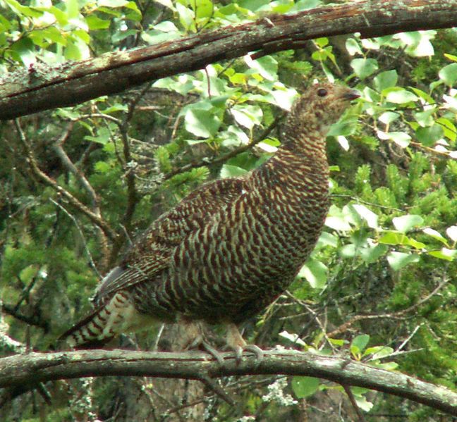
Technical Summary                                                                                     pag. 4

                    Table 3: Average temperature increases in winter and summer seasons for
                   A2 and B2 scenarios in 2020 and 2050; increases are simulated by HadCM3
                                          model for Northern Italy cell.
                                      Winter Summer Winter Summer
                                       2020       2020       2050        2050
                                        (°C)       (°C)       (°C)       (°C)
                                A2      0,84       2,39       2,02       4,83
                                B2      1,54       3,08       1,82       4,42

Areas suitable for their morphological, vegetational and trophic characteristics, may not be suitable
because of their small extension; these areas are not capable of providing individuals with the
minimum necessary space. The suitability map must, thus, be corrected eliminating those areas that,
even if suitable, are too small in extension. On the basis of the alpine ibex ecology, minimum area
dimension is set equal to 400 ha. The number of potential individuals in Parco dell’Adamello under
different scenarios of climate change is listed in Table 4.

                         Table 4: Number of alpine ibex individuals in the baseline and
                                         climate change scenarios.
                                                    Potential individuals
                                                 Winter            Summer
                               Baseline            1.139             1.507
                               A2 – 2020           1.455              862
                               A2 – 2050           1.617              360
                               B2 – 2020           1.612              696
                               B2 – 2050           1.608              416

Results of the analysis clearly show that the ibex population distribution and consistency in Parco
dell’Adamello will be affected by climate change. Precisely, because of the projected increase of
average temperature, the population potential density will slightly increase in the winter and
strongly decrease in the summer. Figure 3 shows the suitability maps, obtained as the output of the
wintering model, for the A2 scenario in 2020 and 2050. Current suitable areas that are projected to
remain suitable in the future are coloured in yellow; current suitable areas that will become
unsuitable are coloured in pink; current unsuitable areas that will became suitable are coloured in
blue. Figure 4 shows output maps of the aestivation model for A2 scenario; as in Figure 3, yellow
areas will remain suitable in the future and pink areas are those that will be lost because they will
become unsuitable. There is a marked contraction of the 2020 suitable area, with a further
worsening in 2050. In future scenarios, the suitable area shifts toward the Eastern side of the Parco
dell’Adamello, where the highest elevations are located. An analogous result is achieved for the B2
scenario.
In the summer, ibex potential density in Parco dell’Adamello decreases from 1,511 individuals to
891 in the best scenario (A2 – 2020) down to 380 in the worst scenario (A2 – 2050); in the winter,
potential density increases from 1,587 to 1,777 in the best scenario (A2 – 2050) and to 1,684 in the
worst scenario (A2 – 2020). The critical season is thus summer: the availability of suitable areas in
this season will act as a bottleneck for the overall ibex individuals in the Parco dell’Adamello.
These are preliminary analysis and the different formulation of the wintering and the aestivation
models may have caused such a dramatic difference between summer and winter potential
populations. Summer distribution depends, in fact, only on altitude. Since climate change causes a
temperature increase, ibex suitable areas move toward higher altitudes and, thus, the suitable area
decreases because it is limited by mountain peak. Even if the structure of the model may influence
the results, it is consistent with what expected to actually happen: species will be able to survive to

Progetto Kyoto Lombardia – Linea Esternalità Ambientali (2008)                Technical Summary - Terzo Anno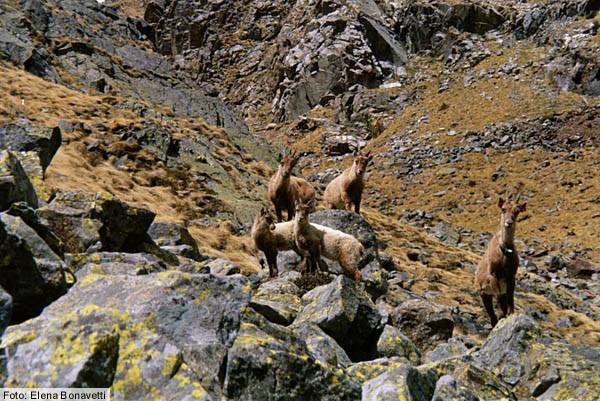
Technical Summary                                                                                                 pag. 5

increased temperatures until they will be able to find, at higher elevations, habitat with climatic (but
not only) suitable characteristics. Model results may be interpreted as follow: the most critical
impacts of climate change in alpine environment will emerge for those species that are sensible to
high temperatures, in particular in the summer season.

 Figure 3: Ibex habitat suitability maps for the winter model in Parco dell’Adamello. Yellow: areas that are currently
suitable and that will remain suitable under GCC; pink: areas that are currently suitable and that will become unsuitable
  under CCG; blue: areas that are currently unsuitable and that will became suitable under CCG. The map on the left
                         refers to A2 – 2020 scenario, the map on the right to A2 – 2050 scenario.

 Figure 4: Ibex habitat suitability maps for the summer model in Parco dell’Adamello. Yellow: areas that are currently
suitable and that will remain suitable under GCC; pink: areas that are currently suitable and that will become unsuitable
           under CCG. The map on the left refers to A2 – 2020 scenario, the map on the right to A2 – 2050.

Progetto Kyoto Lombardia – Linea Esternalità Ambientali (2008)                     Technical Summary - Terzo Anno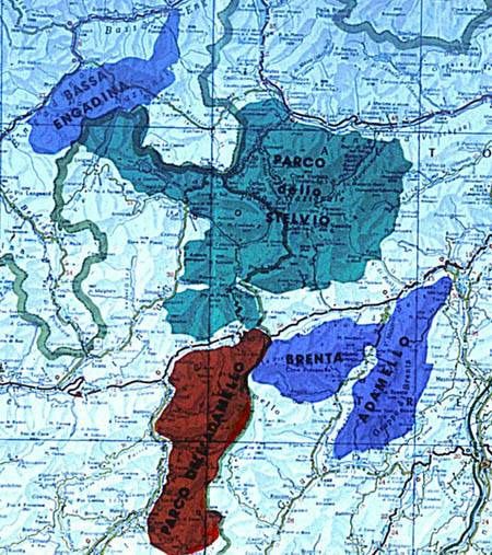
Technical Summary                                                                                      pag. 6

Brown trout (Salmo trutta)
A second climate change impact assessment focuses on an aquatic species: the brown trout (Salmo
trutta; Figure 5) that lives in the upper part of river Adda (Valtellina valley), flowing from Lovero
to lake Como (Figure 6). Aquatic species, such as fishes, are a useful indicator: being an upper
trophic level, they strongly depend on water and flowrate quality. Thus, if it is possible to estimate
alterations of the fish community, it is also possible to evaluate changes of the overall aquatic
environment.
River Adda flow regime is typical of alpine rivers, characterized by low waters in the winter. In the
past, the river flow was naturally shaped by precipitations (abundant in the summer) and by snow
melt during spring. Since 1896, with the construction of many hydro-power stations, catchments
and reservoirs, and with the industrial and agricultural demanding usage of water, the present
regime has considerably changed; in particular, flows are markedly lower all along the river.

                                     Figure 5: Brown Trout (Salmo trutta).

                  Figure 6: Upper river Adda basin; numbers indicate stations for water quality
                                    measurement (ARPA Lombardia, 2003).

The brown trout is a common species in Italy, even if original only in the Alps and in the Northern
part of Apennines. Brown trout prefers cold water mountain streams; thus, habitat is restricted and
limited by specific parameters, such as water temperature, dissolved oxygen, stream velocity and
depth. These traits make the species a good indicator for climate change impacts studies (Mohseni
et al., 2003; Hari et al., 2005).
In order to study climate change impacts on brown trout in the Adda upper river, two variables
sensitive to climate change have been identified: water temperature and river regime. Two distinct
models have been written to predict temperature and flow regime future trends in the presence of
climate change. The first model simulates water temperature under climate change given the current
relation existing between water and air temperature (measured in Villa Tirano and Sondrio
respectively). Future projections for temperature and precipitation under different scenarios of

Progetto Kyoto Lombardia – Linea Esternalità Ambientali (2008)                 Technical Summary - Terzo Anno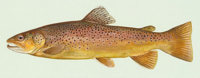
Technical Summary pag. 7
climate change have been derived from the Tyndall Centre for Climate Change Research dataset
(Mitchell et al., 2004). We considered future projection for two emission scenarios (A2 and B2) for
2020, 2050 and 2080. The Tyndall dataset differs from the IPCC dataset for the model output
spatial definition which is 10’. Moreover, the Tyndall Centre offers a dataset for past climatic
variables at the same spatial resolution (10’). For this reason, the two models have been run both in
the past, to produce a baseline scenario, and in the future, to project changes due to climate change.
Emissions scenarios considered are IPCC A1, A2 and B2 in 2020 and 2050; temperature and
precipitation changes are those estimated by the Hadley Centre’s HadCM3 model for the Northern
Italy cell. With these data, we estimated future water temperatures and daily flows and then
calculated suitability indexes under climate change scenarios.
Variazioni di temperatura mensili per il periodo 2050 Variazioni di precipitazioni per il periodo 2050
7
A1Fi
6 A2
1,8
B2 A1Fi
5 1,6 A2
4
B2
[°C]
1,4
f mese
3
1,2
2
1
1
0 0,8
o
e
e
e
zo
no
o
o
io
io
ile
e
br
t
br
gi
br
br
ai
gl
os
ra
tte o
e
ce e
zo
re
no
o
io
ar
fe i o
io
e
r
e
ug
ag
m
m
nn
br
ap
to
r
t
gi
m
lu
br
ril
bb
gl
os
a
b
ra
ag
b
m
ar
ug
tte
ve
gi
ot
ag
m
m
ce
nn
ap
to
m
ge
m
lu
bb
ag
fe
m
0,6
ve
gi
se
no
ot
m
di
ge
se
no
di
Figure 7: Temperature and precipitation average changes for A1Fi, A2 and B2
emission scenarios in 2050 with respect to 1961-1990; projections are from
HadCM3 model for Northern Italy cell.
To study climate change impacts on brown trout, two suitability indexes were used. The first index
is related to the maximum water weekly temperature, because river suitability depends on this
parameter. Habitat suitability varies with maximum weekly water temperature via the function
shown in Figure 8 where the blue curve is for adults and juveniles, and the red dotted curve for fry
(Raleigh et al., 1986). The index value varies between zero (non suitable habitat) and one (optimal
habitat).
The second index deals with low flowrates. A study on the upper river Adda showed that an
increase in flowrate means an increase of usable area for brown trout, and that this increase is not
linear; in particular, the increase is modest for flows over 40 m3/s (Vismara et al., 2001). The 40
m3/s flow is, thus, assumed as the minimum flowrate for brown trout in the upper river Adda, and is
therefore used as reference value to estimate how many days a year the river is not suitable because
of its low flow, through the Imagre index.
Progetto Kyoto Lombardia – Linea Esternalità Ambientali (2008) Technical Summary - Terzo Anno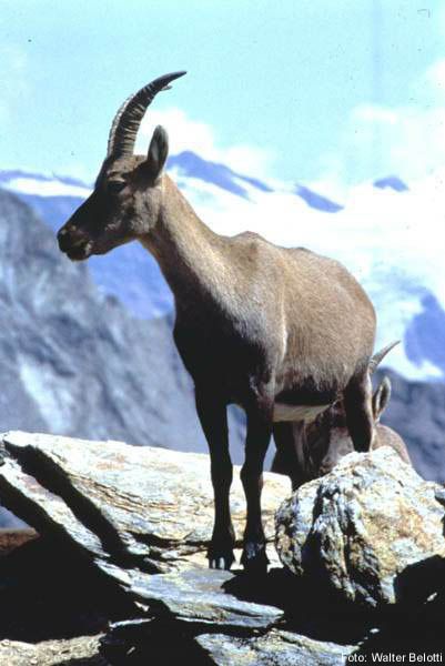
Technical Summary                                                                                                                                           pag. 8

                                               1,2

                                               1,0

                     indice di vocazionalità
                                               0,8

                                               0,6                                                                                    adulti e giovani
                                                                                                                                      avannotti
                                               0,4

                                               0,2

                                               0,0
                                                                         1       6       11       16       21        26       31
                                                                                        T max media settimanale

        Figure 8: Brow trout suitability curves as a function of maximum weekly water temperature;
           blue curve is for adults and juveniles, red dotted curve is for fry (Raleigh et al., 1986).

We estimated the variation of meteo-climatic and hydrological variables under global climate
change scenarios. Weekly average water temperature is estimated through a linear relation between
water and air temperatures. We used measures of water temperature from ARPA in Sondrio for
2000-2006; these are punctual measures, registered once a month, and they do not refer, as
preferable, to an average (daily or monthly) temperature. Air temperature as well refers to measures
in Sondrio for 2000-2005. For each degree of air temperature increase, water temperature increase
is estimated about 0.46°C in Villa Tirano, the hottest station; we assumed that if critical
temperatures are not likely to be registered in Villa Tirano, they should not be expected in other,
cooler, stations as well. Maximum weekly water temperature in baseline and climate change
scenarios were estimated with the following assumptions: the relation found for 2000-2005 remains
valid in the future and also for weekly averages. These simplifying hypothesis are necessary in
order to compensate the scarcity of more detailed measures of water temperature.
The graph in Figure 9 shows the results of the habitat suitability model that utilizes maximum water
temperature. Results show that adults and juveniles (blue bars) will not be affected by increasing
water temperature, since the indexes remain equal to one in all scenarios. Fry, instead, will be
negatively affected by warmer waters (red bars): the suitability index decreases up to 0.8 in the A1
scenario in 2050.
                                                                             1
                                               indice di vocazionalità

                                                                         0,75

                                                                          0,5

                                                                         0,25

                                                                             0
                                                                                 Base         A2 2020     A2 2050         B2 2020   B2 2050
                                                                                                          scenario

                    Figure 9: Values of the suitability index of maximum water temperature for
                         adults and juveniles and for fry under climate change scenarios.

Daily average flow is estimated via a lazy learning algorithm (Birattari e Bontempi, 2003) function
of air temperature and precipitation on the upper river Adda basin. We used air temperature series
measured in Sondrio, precipitation on the upper Adda basin and flowrates in Fuentes; all data are

Progetto Kyoto Lombardia – Linea Esternalità Ambientali (2008)                                                                      Technical Summary - Terzo Anno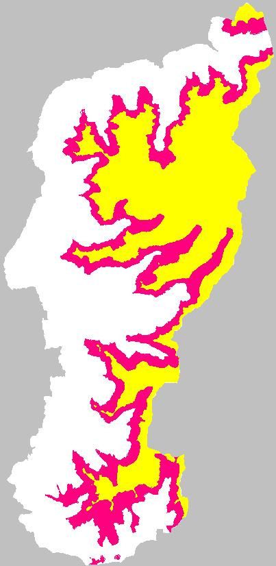
Technical Summary                                                                                    pag. 9

daily averages for 1984-2002. The lazy learning algorithm is applied only after the removal of the
process periodicities. At this purpose, we used a Fourier series decomposition, whose expression
was found after trial and errors and whose parameters were estimated via minimum square
algorithm. Figure 10 shows measured and estimated flowrates. The baseline scenario was obtained
applying the same algorithm, but using as input values measures from 1965 through 1980. This
scenario, thus, can be compared with climate change scenarios because all projections are affected
by the same errors.

                  Figure 10: Measured and simulated flows in validation; data are shown since
                                                march 1998.

The frequency of days with flow below the minimum flowrate doesn’t show marked changes in
future scenarios. While baseline frequency is about 6%, it varies between 4.8% in A2-2050 and 7%
in B2-2050. The low flow frequencies show increases as well as decreases with respect to the
baseline scenario; this is consistent with uncertainties of projected precipitation changes under
climate change in Northern Italy.
We can conclude with the observation that climate change impacts on brown trout in upper river
Adda are estimated to be moderate. The analysis, though, was limited by some critical aspects: first
of all, the scarcity of available data for the models’ calibration (water and air temperature) and their
low quality. Furthermore, upper river Adda is strongly regulated, making more difficult to model
the river regime; a black box model was in fact used to model the river discharge. A conceptual
model would probably allow a better fit and would be capable of including different phenomena
affected by climate change, such as glaciers’ retreat and snowmelt.

Progetto Kyoto Lombardia – Linea Esternalità Ambientali (2008)               Technical Summary - Terzo Anno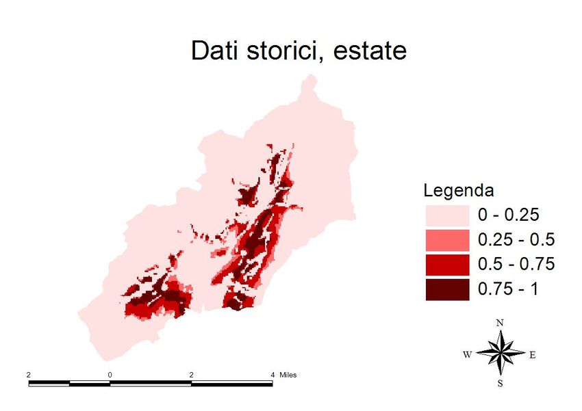
Technical Summary                                                                                            pag. 10

Black grouse (Tetrao tetrix tetrix)
In the Alpine environment, which is characterised by high biodiversity and vulnerability, the
species of the black grouse (Tetrao tetrix) is an important ecological indicator (Wöss e Zeiler,
2003). In January 2008, an European climatic atlas of birds species has been published (Huntley et
al., 2007). Using bioclimatic models, the atlas shows how global climate change will affect species
(such as the black grouse) distribution through a shift of about 550 km towards north-east by the
end of the century, with consequences on habitat availability and biodiversity.
This study focuses on identifying some of the possible impacts of climate change on the black
grouse habitat. In particular, a suitability model is used to study the impacts in the area of Alpe
Devero. As a result of this analysis, we show that the temperature increase will cause a habitat shift.
The black grouse (Figure 11) is a large bird in the grouse family. The species doesn’t have strict
requirements in choosing its habitat; it prefers the upper limit of the forest and, as nesting sites,
vegetation made of small shrubs, rhododendrons and blueberry, which provide food and protection.
It generally avoids dense wood forests. The preferred altitude ranges between 1500 and 2200 m. A
peculiar mating ritual takes place during spring in traditional open areas (arenas) where the males
display making a highly distinctive mating call. The presence of forested slopes is equally important
because it provides suitable habitat to survive to rigid winter conditions (Parco Veglia-Devero,
2006).

             Figure 11: Two male individuals during the mating ritual (left); a female individual (right).

The Parco Naturale dell’Alpe Veglia e dell’Alpe Devero is located in Val d'Ossola (Verbania), the
western limit of Lepontine Alps. The park was established in 1995 and is a protected area of about
10.000 ha. The natural environment is mainly characterized by vast pastures, surrounded by
coniferous forests with rhododendron and blueberry in the underwood. The area of study is the
Conca del Devero, located within the Parco, and has an extension of 56,8 km2 (Figure 12). The
species that distinguish the Alpe Devero are mainly larch (Larix decidua), with undergrowth to
rhododendron (Rhododendron ferrugineum) and black blueberry (Vaccinium myrtillus). The forest
upper limit is at 2000-2200 m; at higher altitudes there are only rhododendron and blueberry that
gradually diminish.

Progetto Kyoto Lombardia – Linea Esternalità Ambientali (2008)                   Technical Summary - Terzo Anno
Technical Summary pag. 11
Figure 12: Geographical location of the Parco Veglia Devero.
The habitat suitability model used in this study has been developed, calibrated and validated for the
Alpe Devero (Ranci Ortigosa, 2000). It is developed on cartographic data (1:10.000 and 1:25.000
scales) of the area and it allows to evaluate the suitability of a specified area at local level. The
model distinguishes separately the environmental features that characterize the spring arenas for the
mating rituals and the areas for the nesting and caring for the chicks. The model results are
expressed in terms of probability of presence of the species. The analysis related to the mating areas
are derived from the counts of both male and female individuals in the arenas. The analysis related
to the nesting areas are derived only from the counts of the female individuals with a nest. The
cartography needed for the development of the two models is listed in Table 5. The analysis has
been restricted only on the Alpe Devero because the vegetation map is not available for the whole
area, but only for this limited part of the park. The model is implemented with ArcGIS 9.1 software.
Table 5: Maps needed for the implementation of the habitat suitability model.
Scale,
Maps References Extension
resolution
Digital elevation model (DEM) Res.50 m Gauss Boaga Digital
Vegetation map for the Alpe Devero 1:25.000 CH1903 Paper
Carta Tecnica Regionale - feature 1:10.000 Gauss Boaga Digital
The habitat suitability model for the black grouse was developed through univariate and
multivariate statistical analysis (Ranci Ortigosa, 2000) in order to study the relationship between the
presence of the species and the environmental variables (elevation, slope, exposure of the slopes,
the presence of rivers and lakes, the presence of cables, the presence of buildings, vegetation types
and a diversity index of the vegetation coverage).
In particular, the suitability highly depends on the maximum altitude and on the vegetation patterns
in both the spring (mating areas; April and May) and the summer models (nesting areas). For the
mating areas the percentage of larch forest are determinant, whilst for the nesting models the
percentage of larch forest together with rhododendron are determinant. The model in formulated as
written in the equation, where the coefficient are described in Table 6:
Progetto Kyoto Lombardia – Linea Esternalità Ambientali (2008) Technical Summary - Terzo AnnoTechnical Summary pag. 12
2
exp(bo + b1 x1 + b2 x1 + b3 x2 )
p= 2
1 + exp(b0 + b1 x1 + b2 x1 + b3 x2 )
Table 6: Regression coefficients for the habitat suitability models (Ranci Ortigosa, 2000).
Spring – mating areas Summer – nesting and feeding areas
Intercept b0 -162.51 Intercept b0 -214.83
Max altitude x1 160.70 Max altitude x1 207.04
Max altitude 2 x 12 - 40.28 Max altitude 2 x 12 -51.78
% larch forest x2 3.77 % larch forest with rhododendron
x2 9.18
The results of the habitat suitability model for the baseline scenario, thus without considering global
climate change, show that there are large areas suitable for the black grouse within the park both in
the spring and in the summer (Figure 13). The most suitable areas are located at the base of the
slopes, at altitudes between 1800 and 2100 m.
Figure 13: Suitability maps for the spring (left) and the summer (right) models under the baseline scenario.
One of the main consequences of climate change is the shift towards higher altitudes in an attempt
to keep in pace with temperature increase. In this case study, two SRES emission scenarios have
been considered (A2 and B2) for three temporal horizon (2020, 2050, 2080); temperature increases
are projected through the HadCM3 AOCGM model (Table 7; IPCC, 2001). Altitude is considered a
proxy for temperature; we assumed that temperature varies with elevation according to a moist
adiabatic lapse rate.
Table 7: Temperature increase (°C) as an average of monthly values.
A2, spring A2, summer B2, spring B2, summer
2020 1,10 0,94 1,28 1,54
2050 1,80 2,88 2,01 2,63
2080 3,96 5,10 2,88 3,87
With a temperature increase of about 1°C, such as those occurring in the spring of 2020 (that is, on
average between 2010 and 2039, for the scenarios A2, +1,095°C, and B2, +1,28°C), the
corresponding altitudinal shift is of about 160 m; results show that for such a shift there is no
excessive loss of habitat. This result seems in line with the argument that the alpine ecosystem can
tolerate, at the local level, temperature increases of about 1-2°C, but can be compromised by further
increases, such as 3-4°C (Theurillat e Guisan, 2001).
The maps in Figure 14 show the results of the spring model for A2 scenario in 2020 and 2050; maps
in Figure 15 show the results of the summer model for A2 scenario in 2020 and 2050. The decrease
Progetto Kyoto Lombardia – Linea Esternalità Ambientali (2008) Technical Summary - Terzo AnnoTechnical Summary pag. 13
of suitable area that occurs for the mating area (spring model) in 2020, although certainly not
negligible, seems to allow the permanence of areas sufficient to host the species. The availability of
suitable area drastically decreases by 2050; at this time, areas with the highest suitability sharply
decrease. With regards to the availability of nesting areas (summer model), there is a lower share of
suitable area in the area already for the baseline scenario. With climate change, the suitable area
sharply decreases already by 2020. Similar results are observed for the B2 emission scenario.
Figure 14: Black grouse suitability maps in the Alpe Devero; spring model, A2
emission scenario.
Figure 15: Black grouse suitability maps in the Alpe Devero; summer model,
A2 emission scenario.
The changes in suitable areas can also be observed by analysing the statistics resulting from the two
implemented models. In particular, Figure 16 and Figure 17 show the percentages of the number of
cells in each probability (of species occurrence) class for each scenario and timeframe, respectively
for the spring and summer models (note that the area upon which statistics are calculated remains
constant as is the area of study, namely the basin of Devero). Climate change impacts on area
suitability are highest for the most suitable classes (those with a probability of species occurrence
higher than 0,5). The share of pixels with probability 0,5÷0,75 dramatically decreases already by
2020; pixels with probability higher than 0,75 disappear by 2050. Global climate change will have a
relevant role impact on the black grouse: the results of the spring and summer models shows that
we can expect a sharp decrease in the suitable area. the existence of the species might be
compromise by habitat reduction.
Progetto Kyoto Lombardia – Linea Esternalità Ambientali (2008) Technical Summary - Terzo AnnoTechnical Summary pag. 14
PRIMAVERA
100%
95%
90% 0,75-1
0,50-0,75
0,25-0,50
85% 0-0,25
80%
75%
Dati storici A2-2020 A2-2050 B2-2020 B2-2050
Figure 16: Share of pixels belonging to each suitability class for the spring model.
ESTATE
100%
95%
90% 0,75-1
0,50-0,75
0,25-0,50
85% 0-0,25
80%
75%
Dati storici A2-2020 A2-2050 B2-2020 B2-2050
Figure 17: Share of pixels belonging to each suitability class for the summer model.
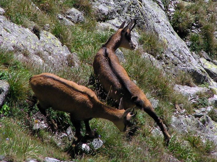
The chamois (Rupicapra rupicapra)
In this case study, we analysed climate change impacts on the chamois (Rupicapra rupicapra)
habitat in Val Chiavenna (Sondrio). The chamois is an important species in the alpine ecosystem;
moreover it is important in the managing of the hunting season. A habitat suitability model for the
chamois is available, whose validity has already been tested for the area in examination (Ranci
Ortigosa 2000; Tosi et al., 1996).
The alpine chamois (Rupicapra rupicapra) is an herbivorous goat that lives in the mountain or sub-
mountain environment (Figure 18). The chamois prefers both the open environments, such as high-
alpine meadows, and the wooded areas. In the winter, the chamois searches for places that offer
repair and have little snow, such as slopes beaten by the wind, steep and sunny slopes, wooded
areas at medium and low altitude.
The Val Chiavenna alpine area extends for 57.603 ha between the Lepontine and the Retiche Alps.
This area is highly mountainous and is characterized by rapid changes of landscape: from hills to
mountains and steep slopes (63% of the area is above 1,500 metres above sea level). A rich and
diverse vegetation covers the area; over a third (39%) of the area is covered with forests, mainly of
deciduous species at lower altitudes and of conifers at higher altitudes. Pastures and prairies cover
about 12% of the area. The chamois is a stable presence in the area, even though with a low density
Progetto Kyoto Lombardia – Linea Esternalità Ambientali (2008) Technical Summary - Terzo AnnoTechnical Summary pag. 15
individuals (Scherini, 1994). The population is estimated to be of about 500÷900 individuals
(census data for the period 1991-1997), whilst the known culls are 4÷9% of population.
Figure 18: The alpine chamois (Rupicapra rupicapra).
The model used to assess the habitat suitability of Val Chiavenna is a model similar to the one used
for the ibex. The habitat suitability model is divided into two models: one is dedicated to evaluate
suitable areas for the winter, the other is dedicated to evaluate suitable areas for the summer. The
wintering model is based on the following environmental variables: altitude, slope, morphological
complexity, land use, assolation. The aestivation model depends on the following environmental
variables: altitude, slope, morphological complexity, land use and aspect. The habitat suitability
function for both the wintering and the aestivation models is given by the sum of the scores given
by all individual environmental variables, as listed in Table 8. The number of potential individuals
that can be sustained by a unit of area depends on the final score of the habitat suitability function
for that unit of area. As listed in Table 9, the density potential ranges from 0 for unsuitable areas to
25 chamois per 100 ha for the most suitable areas. The 98 (104) classes of suitable aestivation
(wintering) suitable areas were divided into 5 classes for clarity, as it is listed in Table 10.
Table 8: Environmental variables for the habitat suitability model for the chamois in Val Chiavenna (Tosi et al., 1996).
Environmental variables Wintering Aestivation Environmental variables Wintering Aestivation
Altitude Slope
(degrees)
2000 13 17
Morphological Assolation (hours/year)
complexity
Nulla 5 5 864-1477 5 -
Bassa 12 12 1477-2090 8 -
Media 24 24 2090-2704 14 -
Elevata 30 30 2704-3317 17 -
3317-3931 20 -
Land use Aspect
Urbanizzato 0 0 Tutte - 10
zone di erosione 0 0 S - 5
bosco ceduo di latifoglie 8 6 SO - 6
bosco di conifere 12 10 SE - 6
Prati 4 4 O - 8
Maggenghi 3 7 E - 8
Progetto Kyoto Lombardia – Linea Esternalità Ambientali (2008) Technical Summary - Terzo AnnoTechnical Summary pag. 16
Environmental variables Wintering Aestivation Environmental variables Wintering Aestivation
pascoli d'alta quota 13 18 NO - 7
incolti erborati 13 11 NE - 7
incolti con cespugli 15 13 N - 7
incolti vegetazione mista 14 12
vegetazione rupestre 20 20
roccia nuda 16 16
Table 9: Potential density of chamois (Tosi et al., 1996).
Potential density Wintering Aestivation
(capi/100 ha) model model
0 0-55 0-45
2 56-60 46-50
4 61-65 51-55
6 66-70 56-60
8 71-75 61-65
10 76-80 66-70
15 81-90 71-75
20 91-100 76-85
25 101-110 86-102
Table 10: Division into six classes of suitability.
Summer Winter
classe 1 1-45 1-55
classe 2 46-55 56-65
classe 3 56-65 66-75
classe 4 66-75 76-85
classe 5 76-85 86-95
classe 6 86-98 96-104
The model is implemented with GIS software; the needed digital cartography comprises the digital
elevation model (DEM) of the soil (slopes and aspects are then derived from the DEM), available
with a 50 m resolution; the vegetation map, derived form CORINE land cover 1:100.000; the
morphological complexity map, derived as a combination of slope and aspect (given by the sum of
the variances of these two variables); the assolation map, derived from slope and exposure maps
together with the number of hours of sun per day over the year (Bartorelli, 1967). For the baseline
scenario, thus without climate change, the maps of suitable areas for the wintering and aestivation
models are in shown Figure 19.
Progetto Kyoto Lombardia – Linea Esternalità Ambientali (2008) Technical Summary - Terzo AnnoTechnical Summary pag. 17
Figure 19: Habitat suitability map for the aestivation (left) and for the wintering
(right) model for the chamois in Val Chiavenna
In order to evaluate the impacts of global climate change of the chamois habitat suitability, two
scenarios have been considered, A2 and B2 chosen within the IPCC emission scenarios. The
temperature variation is derived from the dataset elaborated by the Tyndall Centre for Climate
Change Research, on the basis of the HadCM3 AOGCM model results. The Tyndall dataset
comprises monthly average temperatures at a detailed spatial scale of 10’, both for the baseline
scenario and for future projections (Mitchell et al., 2004). The vertical resolution of the data is 18,5
km at all latitudes, while the horizontal resolution to 45° latitude is 13,1 km. Projected temperature
increases for each scenario and each time horizon under consideration are listed in Table 11.
Table 11: Average temperature increase (°C) for the winter (December, January,
February) and summer (June, July, August) seasons.
A2, winter A2, summer B2, winter B2, summer
2020 0,90 1,41 0,72 1,38
2050 2,07 3,27 1,38 2,62
2080 3,63 5,74 1,87 3,57
Given the moist adiabatic lapse rate that correlates temperature with altitude, it has been possible to
assess how much the temperature increase, due to climate change, affects the chamois habitat
suitability. It is possible to observe some results from the suitability maps (for example, Figure 20
shows the aestivation suitability maps for the A2 scenario): over the years, areas with a high habitat
suitability index (blue-light blue) are projected to decrease, whilst areas with lower habitat
suitability index (green-yellow) are projected to increase. This highlights the impacts of climate
change on the spatial distribution of the chamois in Valchiavenna: with rising temperatures, suitable
areas decrease and, moreover, there is a general decrease in the value of the habitat suitability
indexes.
Progetto Kyoto Lombardia – Linea Esternalità Ambientali (2008) Technical Summary - Terzo AnnoTechnical Summary pag. 18
Figure 20: Suitability maps for the aestivation of the chamois in Val Chiavenna;
A2 scenario in 2020, 2050 e 2080 (left to right).
From the suitability maps for future scenarios it is possible to estimate the potential number of
individuals that can be sustained, through the table that relates habitat suitability index to the
chamois potential number (Table 9). The trend of the potential number of chamois in the years
2020, 2050 and 2080 for scenarios A2 and B2 is listed in Table 12. A slight decrease in the
potential number is projected by the wintering model (from 1278, in the baseline, to 1161
individuals in the worse case). The same result is valid for the aestivation model, where the number
of potential individuals decreases from 2781, in the baseline, to 2242 individuals in the worse case.
Table 12: Number of potential chamois for A2 and B2 scenarios.
Baseline scenario 1278 2781 1278 2781
A2, winter A2, summer B2, winter B2, summer
2020 1244 2631 1251 2406
2050 1214 2312 1235 2242
2080 1161 1767 1214 2633
Climate change impacts on the alpine ibex population dynamics in the Parco del Gran
Paradiso
The aim of this part of the research project is to assess the ecological impacts of climate change on
the dynamic of a charismatic population at local scale; the analysis is carried out with a series of
simulations of possible future behaviour according to different climate change scenarios. There is a
vast literature on environmental impact assessment that investigates impacts at a large spatial scale,
considering a population at its equilibrium. On the other hand, there is limited literature on change
impacts on the dynamic of a population, mainly because of the lack of data necessary to validate
ecological models (Coulson et al., 2001). A further issue is the lack of climate scenarios at a spatial
and temporal scale small enough for ecological analysis; in this study, we propose a method to
derive stochastic series of daily temperature and precipitation at local scale from global climate
models trends. The method is developed in accordance to the IPCC guidelines (IPCC-TGICA,
2007) and returns a description of both daily and annual climatic variability; these results can be
usefully applied not only to ecological studies, but also to other studies, whenever spatially and
temporally detailed climatic projections are needed.
Progetto Kyoto Lombardia – Linea Esternalità Ambientali (2008) Technical Summary - Terzo AnnoTechnical Summary pag. 19
In this case study, we analyzed climate change impacts on the alpine ibex population located in the
Parco del Gran Paradiso. The ibex is a species with a strong symbolic value: it escaped extinction
thanks to the establishment of the first Italian national park, the Gran Paradiso. Moreover, the Gran
Paradiso colony made the ibex restocking feasible: today ibex can be found in many areas all over
the Alps, with a total number of 31.000 individuals (1993 data). The Gran Paradiso ibex colony is
the largest, accounting for 4.000 individuals. Since 1956 ecological data of the ibex population have
been collected by the Park, thus constituting an exceptionally long time series; this has been the
object of many studies, some of which have investigated the relationship between population
dynamics and climatic conditions, e.g.: Jacobson et al., 2004, Bianchi et al., 2006, Corani e Gatto,
2007. This literature provides a valuable knowledgebase for the development of analysis of climate
change impacts. Jacobson et al. (2004) derived from the data of the Gran Paradiso ibex colony a
model that describes the total number of individuals, without distinguishing by ages or sex. The
annual growth rate is affected by the average winter snow depth measured at the meteorological
station in Serrù (2275 m), which is close to the ibex area, and by a factor that includes both climate
(as snow depth) and density. The set of parameters changes according to the average winter snow
depth being above or below a snow threshold, estimated to be 154 cm. The model had been
calibrated and validated using the time series available since 1956; the last 20 years have been used
for the validation, with positive results in terms of the model being able to reproduce the population
dynamic.
Since the ecological models (Jacobson et al., 2004; Corani e Gatto, 2007) that describe the ibex
population dynamic depend on the average winter snow depth, it is necessary to derive from future
emission scenarios and from global circulation models (GCM) the projected snow depth in the area
of interest. GCM supply the trend of statistics over thirty years timeframe (average and standard
deviation) of some climatic variables (e.g., precipitation, minimum and maximum temperature).
Moreover, the projected changes must be applied to local observed statistics in order to estimate
future values for the area of interest more accurate with respect to coarse GCM cells.
Through an autoregressive model, we obtained monthly values for the climatic variables; then,
through a weather generator we derived daily series of the climatic variable to be used as input to
the snow model. The snow model performs a daily balance between accumulated and melted snow;
these terms depend on daily precipitation and on minimum and maximum temperature. Figure 21
schematically describes the method outlined here to obtain future trends of the population of ibex as
a result of climate change on snow depth.
Figure 21: Scheme of the model for the definition of the future snow depth
scenarios derived from global climate change models (GCM) and local
Progetto Kyoto Lombardia – Linea Esternalità Ambientali (2008) Technical Summary - Terzo AnnoTechnical Summary pag. 20
observations. The climatic variables considered are: precipitation (P), minimum
temperature (Tm) and maximum temperature (TM).
For each climate change scenario and for the baseline scenario, one hundred stochastic simulations
were done based on different disturbances (as input of precipitation, minimum and maximum
temperature variables in the monthly models, as input of the same variables in the daily models and,
finally, in the ecological models). The baseline scenario is derived by imposing no trend for the
average temperatures and no change for the average precipitation and the standard deviations, so
that climate projections for this scenario will have the same statistics as in the 1961-1990
timeframe. Observations measured in 1991 have been used as the initial conditions for the climatic
variables, whilst for the demographic simulations the initial conditions are the most recent available
data (2005). To filter the uncertainty of disturbances, the mean and the extreme percentiles are
derived from the whole stochastic simulations. The projections for the snow depth are simulated
until the 2070-2099 timeframe (centered in 2085); while the time horizon for the ibex demographic
simulations is 2050 because of the model performance. Results of the model show that the snow
depth (Figure 22) is projected to dramatically decrease in the future years with respect to the
baseline scenario (without climate change): by 2085 the snow depth will be 10-35 cm, depending
on the scenario (A2 or B2) and on the GCM (HadCM3, CSIRO, CGCM2) versus 70 cm of the
baseline scenario. By 2050, the reduction will be substantial, with average values between 45 and
50 cm. Some GCM also predict a reduction in climate variability; this could result in a lower
frequency of severe winters. Both for the 2070-2099 and the 2040-2069 timeframes, there are
evident climate change impacts on snow depth: the stochastic simulations are well below the
baseline scenario for all the emission scenarios and all the GCM considered.
Figure 22: Results of the simulation of the winter average snow depth; the graph
shows the median snow depth for climate change scenarios and for the baseline.
The two models of the ibex population dynamic shows an initial increase in the number of
individuals common to all scenarios (Figure 23 and Figure 24), this is probably due to the fact that
the initial conditions (relative to 2005) corresponds to a low stage of the population cycle. After a
few years, the number of ibex sharply increases and then, after 2020-2030, stabilizes at about 200-
1000 individuals. The Jacobson et al. (2004) model is more sensitive to the differences between the
different climate scenarios than the Corani and Gatto (2007) model; results of the Jacobson et al.
(2004) model are trajectories more dispersed and with more fluctuations. Moreover, the Jacobson et
al. model is more sensitive to climate variability: for the baseline scenario the range between the
two percentiles is 2500-5500 individuals compared to 2800-4400 individuals for the Corani and
Progetto Kyoto Lombardia – Linea Esternalità Ambientali (2008) Technical Summary - Terzo AnnoTechnical Summary pag. 21
Gatto model. The range of demographic variability as a result of climate change is estimated to be
respectively 2500-6500 individuals and 3000-5000 individuals. There is no trajectory, whatever the
disturbance or the climate scenario, that shows the extinction of the ibex population; the CSIRO-B2
projection reports the worst case, with the lower quantile decreasing to 1500 individuals.
The simulations of ibex population under climate change conditions show an increase in the number
of individuals up to 4000-4800 compared to 3800 in the baseline scenario. The SRES A2 scenarios
project a higher decrease in snow cover than the B2 scenarios; this, in turns, results in a higher
increase of the ibex individuals for the A2 scenarios than in the B2 scenarios, showing that
population dynamic is mainly driven by direct effects of snow depth on mortality.
Figure 23: Statistics (median of the number of individuals) of the ibex simulation for climate
change scenarios and for the baseline scenario with the Jacobson et al. (2004) model.
Figure 24: Statistics (median of the number of individuals) of the ibex simulation for climate
change scenarios and for the baseline scenario with the Corani and Gatto (2007) model.
Progetto Kyoto Lombardia – Linea Esternalità Ambientali (2008) Technical Summary - Terzo AnnoTechnical Summary pag. 22 Much caution should be used when analyzing these projections on the ibex population in the Gran Paradiso National Park. First of all, these results are at odds with recent observation of the ibex population. There is growing evidence that the advance of the growing season affects the quality and the nutritional value of the grasses on which ibex juveniles feed, hence causing an increase in mortality rates. Moreover, the results of the habitat suitability models applied to the ibex in Adamello Park showed a sharp decrease in suitable habitat because of climate change and, thus, a decrease in the number of ibex that can be sustained by the park. It is problematic to use only population dynamic models to assess climate change impacts because the model doesn’t take in account indirect effect that could be critical for the ecological system; indirect climate change impacts should be introduced through specific conceptual models. In particular, it could be very interesting, as a continuation of this research, to use habitat suitability models to estimate the population carrying capacity and then to integrate this results in a population dynamic model in order to consider the increase in intraspecific competition due to the reduction of available resources. Adaptation policies and conclusions The climate system is destined to undergo continuous changes in the next centuries: human activities will continue to impacts the climate system; even if greenhouse gas emissions would abruptly stop, there will still be climatic changes. For this reason, we must take action not only to mitigate emissions, but also to adapt to the inevitable consequences of climate change. Species may respond to changes brought by climate change, in different ways: they can adapt to new conditions; move their lifetimes traits over time or move in space, where conditions are still adequate or have become so; if the environmental changes are sudden and do not allow species to adapt or migrate, species will go extinct at local level and, in the event of changes over the whole area of distribution, at global level. Species and organisms have developed various mechanisms to monitor climatic conditions under which they have adapted to live and reproduce; therefore they are able to adapt "autonomously" to climate change. However, this is a very limited capacity because in the absence of significant evolutionary change (which generally requires tens of thousands of years or more), species depend only on their innate ability to respond to climate change. If suitable habitats disappear or change faster than the population adaptive capacity, species will undergo extinction (Malcolm et al., 1998). It is important to underlie that, at least in this century, evolutionary changes will not play an important role in the adaptation of species to climate change (Malcom and Pitelca, 2000). The conservation of biodiversity, of natural ecosystems and of their functions is essential not only for their intrinsic value and for the services they provide to human society, but also for the strict interactions with the climatic system. The sequestration of carbon by natural vegetation, soil, forests, agricultural areas (the terrestrial biosphere) is, in fact, a key component of the carbon cycle. On the other hand, there are several processes that can turn the biosphere from a sink to a source of carbon: fires, pests, violent floods, heat waves, increased water stress and other extreme events. Administrators and all stakeholders should consider a priority to develop policies and measures to reduce the negative impacts of climate change on biodiversity and ecosystems. In particular, the goal should be to increase ecosystems resilience of thus reduce their vulnerability, so that they can respond and adapt to climate change. The adaptation policies should take into account the high degree of uncertainty associated with climate change and its impacts on ecosystems. Where possible, synergistic positive results should be pursued when developing adaptation policies (so-called win-win policy): for example to promote Progetto Kyoto Lombardia – Linea Esternalità Ambientali (2008) Technical Summary - Terzo Anno
Technical Summary                                                                                 pag. 23

the preservation of an ecosystem and, at the same time, to contribute to greenhouse gas emissions
mitigation through the enhancement of carbon sequestration in the terrestrial biosphere. Policies
should be flexible and able to adapt to situations that rapidly change: climate is no longer one of
environmental constant used to develop conservation measures. Today, under climate change,
attention is focused more on adaptive management, that is based on a dynamic and flexible
approach in which measures are planned, implemented and carefully monitored (Mitchell et al.,
2007; Peterson et al., 1997).

Four key elements for ecosystems adaptation policies can be identified (Mitchell et al., 2007): (1)
reduce the direct impacts; (2) reduce the indirect impacts; (3) increase the resilience, (4) facilitate
changes. The measures that can be taken to implement these policies are described below.

- Direct management of ecosystems in order to reduce impacts. The direct management of
ecosystems refers to situations where intervention, such as changing the microclimate or soil
drainage, can allow organisms to persist in their current location.

- To promote the dispersal of species, and to allow species to move into new areas with a suitable
climate. Measures that have been proposed include the establishment of ecological corridors and
stepping stones that connect the main patches of the habitat. At the same time, we must improve the
quality of environmental matrix in which the patches are. The implementation of this strategy
strongly depends on species and habitat characteristics. The ecological corridors can also encourage
undesired effects, such as the spread of invasive species; in this case, monitoring and counter-
measures are essential.

- To increase the available habitat, both by enlarging existing patches or by creating new ones, in
order to favours the increase of resilience. On the one side, it increases the population size, on the
other it increases the diversity of climates and, therefore, there are more possibilities that there will
be suitable areas even under climate change.

- To reduce pressures other than climate change. In order to reduce ecosystems and species
vulnerability, it is of major concern to pursue the reduction of all those impacts that are not directly
linked to climate change (eg, water and air pollution, fertilizer and chemical compounds leakages,
habitats fragmentation, land use change).

As already mentioned, together with adaptation policies, a long term monitoring of the results of the
policies implemented should be carried out. It is also important to monitor climate change and its
impacts on species and ecosystems. Obviously, without monitoring, it would not be possible to
evaluate the success (or failure) of the implemented measures, and to adjust them in order to make
them as much effective as possible.

Finally, the importance of the availability of a robust knowledge base of climate change and of its
impacts on species and ecosystems is stressed out. Without this knowledge, the design of effective
adaptation policies becomes more and more complicated. It is important to reduce the uncertainties
and to increase the understanding of the processes that drive changes and to further develop the
ability to estimate projected changes. Unfortunately, to date, this knowledge base in Lombardy, and
in Italy in general, is rather fragile. In Italy, Alps are the only areas from which data are considerate
reliable by IPCC’s AR4; according to IPCC (Parry et al., 2007) data are deemed reliable if they
derive from at least 20 years long studies and if they show significant changes even in disagreement
with global climate change. There is lack of impacts assessment on biological systems throughout
the rest of the national territory. This shows a serious weakness in a country that is in the list of
global biodiversity hotspots, both terrestrial (Myers et al., 2000) and marine (Bianchi and Morri,
2000).

Progetto Kyoto Lombardia – Linea Esternalità Ambientali (2008)          Technical Summary - Terzo Anno
You can also read