Projected Shifts in 21st Century Sardine Distribution and Catch in the California Current
←
→
Page content transcription
If your browser does not render page correctly, please read the page content below
ORIGINAL RESEARCH
                                                                                                                                               published: 19 July 2021
                                                                                                                                     doi: 10.3389/fmars.2021.685241

                                            Projected Shifts in 21st Century
                                            Sardine Distribution and Catch in the
                                            California Current
                                            Jerome Fiechter 1* , Mercedes Pozo Buil 2,3 , Michael G. Jacox 3,4 , Michael A. Alexander 4
                                            and Kenneth A. Rose 5
                                            1
                                              Ocean Sciences Department, University of California, Santa Cruz, Santa Cruz, CA, United States, 2 Institute of Marine
                                            Sciences, University of California, Santa Cruz, Santa Cruz, CA, United States, 3 Environmental Research Division, Southwest
                                            Fisheries Science Center (NOAA), Monterey, CA, United States, 4 Physical Sciences Laboratory, National Oceanic
                                            and Atmospheric Administration (NOAA), Boulder, CO, United States, 5 Horn Point Laboratory, University of Maryland Center
                                            for Environmental Science, Cambridge, MD, United States

                                            Predicting changes in the abundance and distribution of small pelagic fish species
                                            in response to anthropogenic climate forcing is of paramount importance due to
                          Edited by:        the ecological and socioeconomic importance of these species, especially in eastern
                     Chih-hao Hsieh,
                                            boundary current upwelling regions. Coastal upwelling systems are notorious for the
    National Taiwan University, Taiwan
                                            wide range of spatial (from local to basin) and temporal (from days to decades)
                         Reviewed by:
                         Evan Howard,       scales influencing their physical and biogeochemical environments and, thus, forage
             University of Washington,      fish habitat. Bridging those scales can be achieved by using high-resolution regional
                          United States
                            Chen-Yi Tu,     models that integrate global climate forcing downscaled from coarser resolution earth
         Institute for National Defense     system models. Here, “end-to-end” projections for 21st century sardine population
       and Security Research, Taiwan
                                            dynamics and catch in the California Current system (CCS) are generated by coupling
                  *Correspondence:
                                            three dynamically downscaled earth system model solutions to an individual-based
                      Jerome Fiechter
                   fiechter@ucsc.edu        fish model and an agent-based fishing fleet model. Simulated sardine population
                                            biomass during 2000–2100 exhibits primarily low-frequency (decadal) variability, and
                   Specialty section:
         This article was submitted to
                                            a progressive poleward shift driven by thermal habitat preference. The magnitude of
Global Change and the Future Ocean,         poleward displacement varies noticeably under lower and higher warming conditions
               a section of the journal     (500 and 800 km, respectively). Following the redistribution of the sardine population,
          Frontiers in Marine Science
                                            catch is projected to increase by 50–70% in the northern CCS and decrease by 30–
           Received: 24 March 2021
            Accepted: 16 June 2021          70% in the southern and central CCS. However, the late-century increase in sardine
            Published: 19 July 2021         abundance (and hence, catch) in the northern CCS exhibits a large ensemble spread
                              Citation:     and is not statistically identical across the three downscaled projections. Overall, the
               Fiechter J, Pozo Buil M,
        Jacox MG, Alexander MA and
                                            results illustrate the benefit of using dynamical downscaling from multiple earth system
      Rose KA (2021) Projected Shifts       models as input to high-resolution regional end-to-end (“physics to fish”) models for
  in 21st Century Sardine Distribution      projecting population responses of higher trophic organisms to global climate change.
  and Catch in the California Current.
            Front. Mar. Sci. 8:685241.      Keywords: climate projection, dynamical downscaling, California Current, sardine fishery, end-to-end ecosystem
     doi: 10.3389/fmars.2021.685241         model, upwelling system

Frontiers in Marine Science | www.frontiersin.org                                  1                                              July 2021 | Volume 8 | Article 685241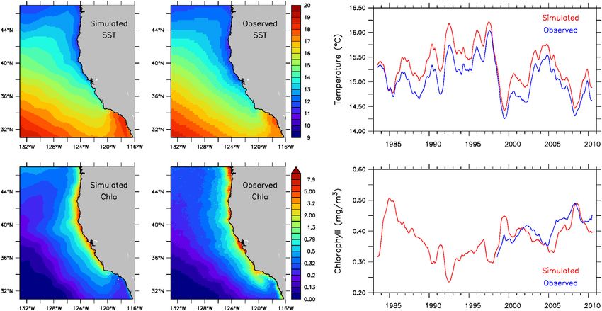
Fiechter et al.                                                                                           California Current Sardine Climate Projections

INTRODUCTION                                                                  The focus of this study is to extend the dynamical downscaling
                                                                           approach of Pozo Buil et al. (2021) to sardine population
In eastern boundary current upwelling regions, such as the                 dynamics and catch in the CCS by integrating a full life-cycle
California Current System (CCS), sardines and other small                  individual-based model (IBM) for sardine and an agent-based
pelagic fish play a key role in the transfer of energy between             model for its fishing fleet into the projections. By nature, the
planktonic organisms and higher trophic levels species, such               IBM allows for a mechanistic interpretation of environmental
as seabirds and marine mammals (Cury et al., 2000; Peck                    drivers regulating growth, reproduction, survival, and behavior
et al., 2021). Healthy sardine populations also account for                of sardine (Fiechter et al., 2015; Rose et al., 2015), and it
a substantial fraction of the global fish catch (Fréon et al.,             is thus well-suited to explore which and how underlying
2005) and support important commercial fishing activities                  physical and biological processes will likely cause changes in
worldwide, yielding multimillion dollars ex-vessel revenues                sardine abundance and distribution over the course of the 21st
(i.e., revenues from landed catch) off the west coast of the               century. While anthropogenic warming will undoubtedly play an
United States alone (Pacific Fishery Management Council                    important role (Cheung et al., 2015; Morley et al., 2018), the IBM
(PFMC), 2011). The ecological and economic significance of                 projections can shed light on the relative extent to which future
sardines in upwelling regions make them a prime candidate                  temperatures will affect sardine population dynamics through
to explore how populations may respond to changing climate                 metabolism (growth, reproduction, and early life survival rates)
conditions (Cheung et al., 2015; Morley et al., 2018) and to               and movement behavior (shift in thermal habitat). The IBM also
identify potential drivers (e.g., warming and prey availability) and       offers insight into the possible influence on sardine of other
uncertainty sources (Frölicher et al., 2016) associated with shifts        bottom-up drivers, such as coastal upwelling intensity and prey
in distribution and abundance.                                             availability, which may exhibit more subtle local and regional
    Environmental variability in the CCS occurs over a wide                responses to climate change (Rykaczewski et al., 2015; Checkley
range of spatiotemporal scales and is seasonally driven by coastal         et al., 2017) or whose trends have not yet emerged from natural
upwelling of cool, nutrient rich waters in response to prevailing          variability (Brady et al., 2017). Since climate models have inherent
alongshore winds (Checkley and Barth, 2009). The combination               physical and biogeochemical uncertainty (Frölicher et al., 2016),
of coastal and curl-driven upwelling produces elevated levels of           the robustness of sardine population and catch projections are
new production along most of the west coast of the United States           assessed by downscaling three representative members of the
and contributes to shaping the habitats of planktonic organisms            CMIP5 ensemble (Bopp et al., 2013).
and forage fish (Rykaczewski and Checkley, 2008; Zwolinski
et al., 2011; Fiechter et al., 2020). Physical, biogeochemical and
ecosystem states in the CCS are further modulated by basin-                MATERIALS AND METHODS
scale variability associated with ocean-atmosphere couplings,
such as the El Niño Southern Oscillation (Lynn and Bograd,                 End-to-End Ecosystem Model
2002), Pacific Decadal Oscillation (Mantua et al., 1997) and North         The numerical framework is an existing end-to-end ecosystem
Pacific Gyre Oscillation (Di Lorenzo et al., 2008). These decadal          model that has already been successfully implemented to study
changes in environmental conditions have been postulated                   historical sardine and anchovy population variability and their
as the main drivers of low-frequency variability of sardine                environmental drivers in the CCS (Fiechter et al., 2015; Rose
and anchovy populations in the region (Chavez et al., 2003;                et al., 2015; Politikos et al., 2018; Nishikawa et al., 2019) and in
Lindegren et al., 2013).                                                   the Canary Current upwelling system (Sánchez-Garrido et al.,
    The combined effects of basin-scale forcing, regional                  2018, 2021). The end-to-end model includes a regional ocean
processes, and local upwelling patterns on small pelagic fish              circulation component, a nutrient-phytoplankton-zooplankton
habitat pose a significant challenge for predicting how sardine            (NPZ) component, a sardine population dynamics IBM
population dynamics will be affected by changing climate                   component, and an agent-based fishing fleet component. Since
conditions in the CCS and in other eastern boundary current                detailed descriptions of the model can be found in Rose et al.
upwelling systems. Global projections from Earth System Models             (2015) and Fiechter et al. (2015), only an abbreviated overview of
(ESMs) typically lack the necessary atmospheric and oceanic                the different model components is provided here.
horizontal resolution to reproduce the full spectrum of processes              The ocean circulation model is an implementation of the
associated with wind-driven coastal upwelling (Stock et al.,               Regional Ocean Modeling System (ROMS) (Shchepetkin and
2011; Small et al., 2015). Higher-resolution regional models can           McWilliams, 2005; Haidvogel et al., 2008) for the broader
resolve finer-scale physical and biogeochemical coastal dynamics           California Current region (30◦ N to 48◦ N and 116◦ W to 134◦ W),
but must be driven by realistic localized representations of               with a horizontal grid resolution of 1/10◦ (ca. 10 km) and 42
future climate forcing. Dynamical downscaling of low-resolution            non-uniform terrain-following vertical levels. The NPZ model
(∼1◦ × 1◦ ) ESM solutions has emerged as a valuable method for             is a customized version of the North Pacific Ecosystem Model
producing higher-resolution (∼0.1◦ × 0.1◦ ) regional projections           for Understanding Regional Oceanography (NEMURO) (Kishi
of environmental and ecosystem variability in eastern boundary             et al., 2007) specifically parameterized for the CCS (Fiechter et al.,
current upwelling systems under anticipated future conditions              2018, 2020). Physical transport of NPZ tracers is achieved by
(Echevin et al., 2012; Machu et al., 2015; Howard et al., 2020a;           solving an advection-diffusion equation at every time step using
Pozo Buil et al., 2021).                                                   archived daily velocities and mixing coefficients from ROMS. The

Frontiers in Marine Science | www.frontiersin.org                      2                                          July 2021 | Volume 8 | Article 685241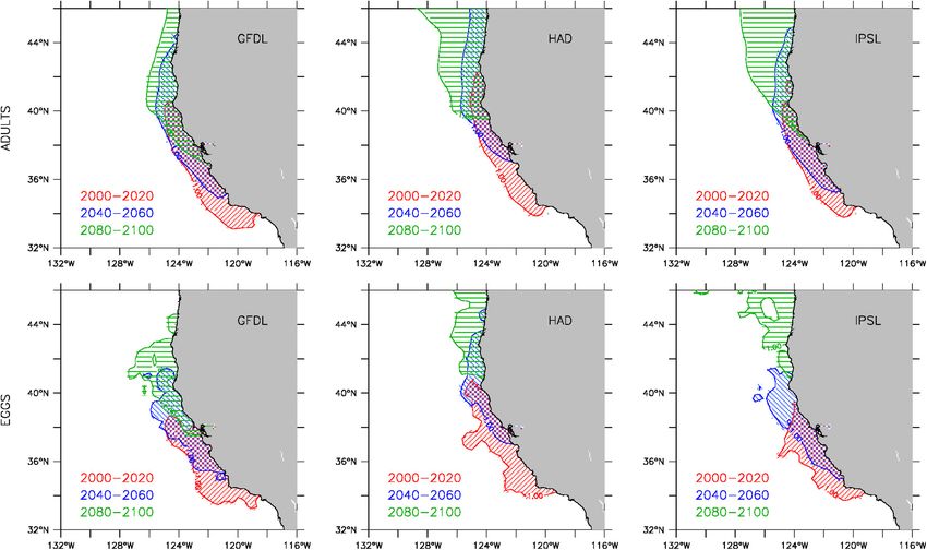
Fiechter et al.                                                                                            California Current Sardine Climate Projections

IBM tracks sardine individuals on the ROMS grid in continuous                the NPZ component, and finally the fish and fleet components.
(Lagrangian) space and over their full life cycle.                           When using archived daily fields, the offline approach yields a
    Scaling from individuals to the population level is done                 solution virtually identical to that of the fully coupled model, yet
using a super-individual approach (Scheffer et al., 1995), where             it allows for larger time steps for the NPZ (dt = 30 min) and
each super-individual in the IBM represents a larger number                  fish and fleet (dt = 6 h) components compared to that of the
of individuals (called worth) with identical attributes (a super-            physical and, hence fully coupled model (dt = 10 min); (ii) The
individual can be envisioned as a school of identical fish). Super-          fish IBM component includes only one coastal pelagic species,
individuals remain in the simulation until they either reach their           sardine, and no migratory predator. Earlier results from Rose
oldest allowed age (10 years) or mortality sources reduce their              et al. (2015) demonstrated that sardine and anchovy had small
worth to zero. All output from the IBM is scaled by the worths               direct effects on each other in the simulations (i.e., dynamics were
of super-individuals (for example, population abundance is the               quasi-independent and therefore separable) and that predatory
sum of the worths over all super-individuals, and mean length is             mortality was small compared to the other sources of mortality
a weighted average of the lengths of super-individuals with the              represented in the model; (iii) The diet for adult sardine has been
weighting factors being their worths).                                       adjusted to include higher feeding preferences on copepods and
    The IBM explicitly includes formulations for growth from                 euphausiids. This modification yields a more realistic offshore
bioenergetics and feeding on zooplankton prey (from NPZ                      extent of the sardine population (food is one of the movement
component), reproduction, and natural and fishing mortality for              cues) compared to that calculated in earlier implementations
the following life stages (as appropriate): eggs, yolk-sac larvae,           of the model where adult sardine favored microzooplankton.
feeding larvae, juveniles, non-mature adults, and mature adults.             The new parameterization also leads to an emergent northward
The development of eggs and yolk-sack larvae is determined                   summer feeding migration (albeit of reduced amplitude and
uniquely by temperature; larvae transition to juveniles based                limited to older fish), thereby alleviating the need of a prescribed
on a weight threshold; juveniles become non-mature adults on                 seasonal migration as in Rose et al. (2015) and Fiechter et al.
January 1 of each model year; and adults reach maturity based                (2015). (iv) The parameterization of the NPZ component was
on a length threshold. Since mature adults produce eggs which                revisited to improve the representation of key phytoplankton and
become the next spawning adults, recruitment is an emergent                  zooplankton functional groups in the CCS, especially euphausiids
property in the model (as opposed to being imposed annually or               (Fiechter et al., 2018, 2020). Specific parameter values for the
defined a priori via a spawner-recruit relationship). Behavioral             NPZ, sardine IBM, and fishing fleet models are provided as
movement for juveniles and adults includes temperature and                   supplementary material and references for parameter sources are
consumption cues using a kinesis approach that combines inertial             available in Rose et al. (2015).
and random displacements based on a proximity to optimal
conditions (Humston et al., 2004; Watkins and Rose, 2013).
When temperature and feeding conditions experienced by an                    Historical Simulation and Climate
individual are within a prescribed suitable range (defined here              Projections
as within one standard deviation from the optimal value), the                Four different numerical simulations of the end-to-end model
inertial component is weighted more heavily than the random                  were performed: a historical run for 1983–2010 and three
component, thereby allowing the individual to maintain itself                downscaled climate projections for 1983–2100 based on the
within a suitable thermal and foraging habitat by conserving its             GFDL-ESM2M (Dunne et al., 2012), IPSL-CM5A-MR (Dufresne
current heading and slowing down.                                            et al., 2013), and Hadley-GEM2-ES (Collins et al., 2011) earth
    The fishing fleet model simulates daily fishing trips of boats           system models under the Representative Concentration Pathway
out of 4 United States west coast ports (San Pedro, Monterey,                (RCP) 8.5 emission scenario. These models were selected for
Astoria and Westport). Choice of fishing locations and associated            their inclusion of marine biogeochemical fields and to represent
daily sardine catch are based on a simplified multinomial logit,             the spread of physical and biogeochemical futures in the CMIP5
agent-based approach where boats maximize their expected net                 ensemble: GFDL has a low rate of warming and increased
revenue for each trip (e.g., Eales and Wilen, 1986). While the               primary production; Hadley has a high rate of warming and
fleet model incorporates effort in the sense that no fishing                 decreased primary production; and IPSL corresponds to a
occurs on a given day if a boat does not have access to fishing              moderate scenario (Bopp et al., 2013; Pozo Buil et al., 2021).
locations yielding a positive revenue, it does not account for               The primary purpose of the historical simulation was to generate
specific fisheries management actions that have been imposed                 a reference solution for the calibration and evaluation of the
historically. For example, the simulations do not include the                sardine IBM and fishing fleet model.
regulatory quotas imposed on the fishery during 1986–1991                       For the historical simulation, initial and open boundary
following the sardine moratorium in California (Wolf, 1992) or               conditions for physical variables are derived from the Simple
the lack of a recent commercial fishery in the Pacific Northwest             Ocean Data Assimilation (SODA) reanalysis (Carton and Giese,
until 1999 (Emmett et al., 2005).                                            2008), and surface atmospheric fields are based on version 1 of the
    The version of the end-to-end model used here differs from               Cross-Calibrated Multi-Platform (CCMP1) winds (Atlas et al.,
its earlier implementation in several ways. (i) For computational            2011) and version 5 of the European Centre for Medium-Range
efficiency, each component of the system is run in successive steps          Weather Forecasts (ERA5) reanalysis (Hersbach et al., 2020).
(i.e., offline coupling), starting with the physical circulation, then       Initial and boundary conditions for nitrate and silicic acid are

Frontiers in Marine Science | www.frontiersin.org                        3                                         July 2021 | Volume 8 | Article 685241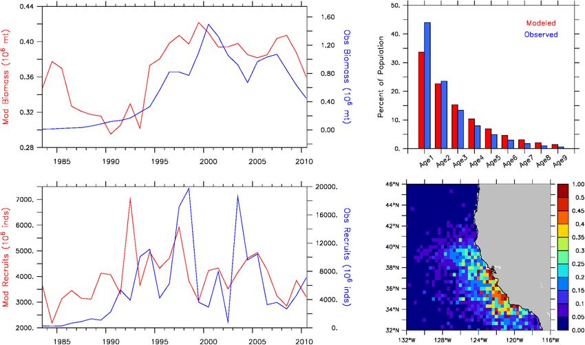
Fiechter et al.                                                                                         California Current Sardine Climate Projections

derived from the World Ocean Atlas (WOA) (Conkright and                   calculated as the standard deviation between the three projections
Boyer, 2002), while other biogeochemical tracers are set to a             and the multi-model mean, (2) spatial distributions of adult
small value (0.1 mmol N m−3 ) for lack of better information.             sardine abundance and egg production, (3) spatial maps of
Total sardine population biomass is initialized so that the biomass       suitable thermal and feeding habitats, and (4) total annual
contributed by mature (age-2 and older) adult individuals at the          catch in the southern (San Pedro), central (Monterey) and
beginning of the simulation roughly matched the mean spawning             northern (Astoria and Westport) CCS. Since sardines in the
stock biomass estimated for 1985–1999 (∼0.35 million metric               model consume multiple prey types from the NPZ component,
tons) (Hill et al., 2010). Sardine super-individuals are randomly         a functional response is applied to combine them into a
initialized within a subregion of the model between 30–35◦ N and          single index (Rose et al., 2015). The functional response
within 100 km of the coast where surface temperatures and food            uses the prey biomasses, and after accounting for feeding
availability on 1 January 1983 are within one standard deviation          preferences and efficiencies of sardine, generates the fraction of
of their respective optimal values for kinesis.                           maximum possible consumption rate that would be achieved
    For the downscaled projections, a “time-varying delta”                (hereafter referred to as “P”). The identification of thermal
method is used to generate open boundary and surface                      and feeding habitats is purposedly based on the parameters
atmospheric forcing. For each ESM, time-varying deltas                    used in kinesis to weight inertial and random movement, so
(representing monthly open boundary and surface atmospheric               spatial changes in projected sardine distributions are directly
anomalies) are calculated relative to their respective 1980–2010          relatable to future availability of suitable conditions in the
climatology and added to their corresponding climatology in               CCS as perceived by individuals in the IBM. Suitable thermal
the historical simulation (SODA and WOA for physical and                  and feeding habitats are thus defined as grid cell locations
biogeochemical open boundary conditions, and CCMP1 and                    where temperature and P values are, respectively, within one
ERA5 for surface atmospheric forcing) (Pozo Buil et al., 2021).           standard deviation of their optimal value, (i.e., 11–16◦ C for
The downscaled projections are generated for 1983–2100 using              temperature and greater than 0.75 for P). For these ranges, habitat
historical forcing for 1983–2005 and the RCP8.5 emission                  quality is highest and inertial movement (indicative of good
scenario for 2006–2100. The main advantage of using a time-               habitat) outweighs random behavior (indicative of poor habitat)
varying delta method is that it corrects for inherent biases in           in kinesis.
the earth model solutions and produces continuous projections                Total biomass is calculated by multiplying the body weight
reflecting climate change effects in the CCS throughout the 21st          by the worth of a super-individual and summing over all super
century (as opposed to the more common “fixed delta” method               individuals representing mature adult sardines; worth is the
that considers only a specific period of the future climate,              number of actual fish represented by a super-individual and
e.g., 2070–2100). The initial location and biomass of sardine             body weight is identical for all fish within a super-individual.
individuals for the projections is determined using the same              Spawning stock biomass is further calculated by summing only
approach as for the historical simulation.                                over super-individuals representing age-2 and older mature adult
                                                                          sardines. Spatial distributions of abundance are calculated as
Analysis                                                                  yearly averages of instantaneous (every 5 days) summed adult
Evaluation of the end-to-end historical simulation includes sea           worth in each grid cell, and egg production is determined by
surface temperatures and surface chlorophyll concentrations               annually summing the number of eggs spawned (scaled up for
from the ROMS and NPZ models; sardine spawning stock                      the worths of spawners) in each grid cell. Adult abundance
biomass, age-class structure, recruitment, and egg distribution           and egg production are subsequently mapped to a coarser
from the IBM; and regional annual catch from the fishing                  30 km resolution grid, which helps smooth out spatial variability
fleet model. Simulated sea surface temperatures and chlorophyll           in the model output not associated with coherent circulation
concentrations are respectively compared to NOAA’s OISST                  features. Total annual catch is calculated by summing daily
AVHRR dataset1 and NASA’s SeaWiFS dataset.2 Simulated                     catch over all boats and all days of the year for each port.
sardine spawning stock biomass (age-2 and older individuals),             An unpaired, two-sample Student’s t-test is also performed on
age-class structure and recruitment are compared to stock                 sardine abundances at each grid cell location to determine if the
assessment estimates from Table 10 in Hill et al. (2010); egg             means of the distributions are statistically identical across the
distribution patterns are evaluated against in situ observations of       three downscaled solutions over the analysis period (2000–2100).
egg presence from Zwolinski et al. (2011); and simulated catch is         The projections are considered statistically “robust” at a grid cell
compared to reported regional United States west coast landings           location if the pairwise (GFDL-Hadley, GFDL-IPSL, and Hadley-
from Table 1 in Hill et al. (2010). Recruitment is an emergent            IPSL) t-tests support the hypothesis of identical means at the 95%
property in the IBM and represents the number of eggs that                confidence level.
survive to enter the adult stage on January 1 of each year.
    Analysis of the end-to-end model projections includes: (1)
total annual adult sardine biomass from each downscaled                   RESULTS
solution and multi-model mean, as well as multi-model spread
                                                                          Model Evaluation
1
    https://www.ncdc.noaa.gov/oisst                                       The evaluation of the ROMS and NPZ models focuses on
2
    https://oceancolor.gsfc.nasa.gov/data/seawifs                         sea surface temperatures and chlorophyll concentrations, as

Frontiers in Marine Science | www.frontiersin.org                     4                                         July 2021 | Volume 8 | Article 685241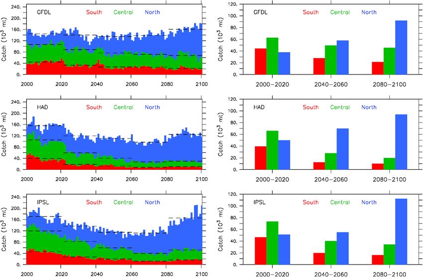
Fiechter et al. California Current Sardine Climate Projections
these two variables are intimately related to the presence of formulations of differing strength. An option for additional
suitable thermal and feeding habitats for sardine individuals analyses would be to calibrate the density-dependence to match
in the IBM. Despite a slight warm bias (∼0.5◦ C or less), the historical spawner-recruit relationship (e.g., from stock
simulated surface temperatures adequately reproduce observed assessment estimates), but it is not clear how this relationship
spatial patterns and temporal variability, including the transition may change under future conditions. Furthermore, since relative
from a warmer to a colder regime in the northeast Pacific changes in simulated sardine abundance and distribution are
Ocean in 1999 associated with a phase change of the Pacific comparable over an order of magnitude change in initial
Decadal Oscillation (Peterson and Schwing, 2003) (Figure 1, population biomass (Supplementary Figure 1), discrepancies in
upper panels). Simulated surface chlorophyll concentrations historical spawning stock biomass and recruitment should not
also demonstrate reasonable agreement with observed values in fundamentally alter the qualitative spatial and temporal patterns
the spatial extent of the coastal upwelling zone and in their identified in the IBM projections.
interannual variability and trend (Figure 1, lower panels). Comparing simulated catch to observed landings is obscured
Historical sardine spawning stock biomass from the by the fact that the fleet model does not account for the sardine
IBM exhibits low-frequency variability comparable to stock moratorium (1974–85) and subsequent period of limited fishing
assessment estimates, with a rapid increase in biomass starting in quotas (1986–1991) in California (Wolf, 1992) and for the lack
the early 1990s, a period of peak biomass during the late 1990s of a recent commercial fishery in the Pacific Northwest until
and early 2000s, and a decline in the late 2000s (Figure 2, upper 1999 (Emmett et al., 2005). Excluding those periods and ramp-
left panel). However, simulated values greatly underestimate up phase of the fishery, simulated catch reasonably reproduces
the difference between high and low biomass periods. Over the the magnitude and temporal variability of reported landings
28 years, simulated values vary by a factor of about 1.5 times in the southern CCS during 2000–2010 and northern CCS
compared to an order of magnitude difference for observed during 2002–2010 (Supplementary Figure 2). However, the
biomass. This discrepancy is partly explained by lower average model exhibits significantly less similarity with landings in the
recruitment values (∼4,200 vs. ∼7,400 million individuals during central CCS, both in amplitude and year-to-year variation.
1990–2010) and smaller interannual variability. The model The agreement between simulated catch and landings (at least
predicts a factor of 2–3 times between high and low recruitment for San Perdo, Astoria, and Westport) during the period of
years, whereas the factor is 5–10 times for recruitment reported high sardine abundance suggests that, despite the factor 2–3
in the stock assessment (Figure 2, lower left panel). However, the difference between simulated spawning stock biomass and stock
IBM reasonably replicates periods of high and low recruitment in assessment estimates, the model results are informative with
the stock assessment, with correlation coefficients of 0.41 based careful interpretation and caveats.
on annual values and 0.71 based on 3-year running mean values.
Furthermore, the IBM provides an acceptable representation Downscaled Projections
of the observed age-class structure of the population, and All three downscaled climate projections display substantial low-
adequately reproduces the observed latitudinal range (33–36◦ N) frequency variability in sardine biomass over the course of the
and offshore extent of sardine spawning based on in situ egg 21st century, with a notable decrease in adult biomass during
presence reported by Zwolinski et al. (2011) for 1998–2009 2020–2040 and a rapid increase in adult biomass starting in the
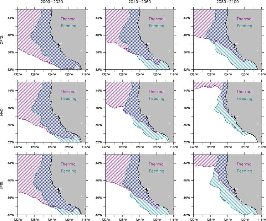
(Figure 2, right panels). 2070s (Figure 3). However, the importance of the mid-century
The cause for the order of magnitude discrepancy between low biomass period and the magnitude of the end of the century
the model and stock assessment during periods of higher and increase differ markedly between the three projections. Based
lower spawning stock biomass is difficult to pinpoint exactly, on the multi-model mean, sardine biomass decreases by about
but prey availability and density-dependent mortality could 40% between historical (2000–2020) and mid-century (2040–
both play a role. The quadratic natural mortality term in the 2060) values, with GFDL projecting a smaller decrease (∼15%)
NPZ component prevents large fluctuations in phytoplankton than the multi-model mean, and Hadley and IPSL projecting a
and zooplankton biomasses [as identified for simulated krill in larger decrease (up to 70% for IPSL). Comparatively, the change
Fiechter et al. (2020)], which could in turn have a stabilizing in sardine biomass during the second half of the century is
effect on recruitment via larval and juvenile growth, and on more substantial, as evidenced by the 2.5–3 times increase in
egg production via adult growth. Introducing density-dependent the multi-model mean between mid-century and end of the
processes (either via mortality such as predation or crowding century values. Individual projections also exhibit greater spread,
effects on prey availability and growth) would presumably with GFDL and Hadley projecting a lower increase (closer to
improve the IBM’s ability to reproduce observed population- doubling), and IPSL projecting a much larger increase (∼7
level patterns in spawning stock biomass. However, density- times increase).
dependence was ultimately not included in the IBM to maximize The projected changes in total biomass are also accompanied
simulated responses to variation in environmental variables by a regional redistribution of the sardine population over
and prey availability, thereby enabling more easily interpretable the course of the 21st century, as illustrated by the poleward
results in the projections. Including density-dependence would shift in the multi-model mean between 2000–2020, 2040–2060,
dampen responses and, given the uncertainty in how to formulate and 2080–2100 (Figure 3). While the poleward displacement
the density-dependence among processes and life stages (see of the sardine population is a common feature of all three
Rose et al., 2001), would require extensive testing of alternative downscaled projections, the timing and magnitude of the shift
Frontiers in Marine Science | www.frontiersin.org 5 July 2021 | Volume 8 | Article 685241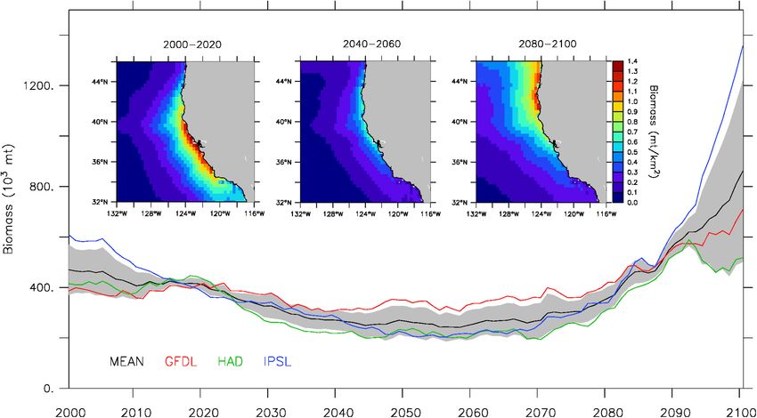
Fiechter et al.                                                                                                              California Current Sardine Climate Projections

  FIGURE 1 | Historical surface temperatures (◦ C) (top) and chlorophyll concentrations (mg/m3 ) (bottom) from the ROMS and NPZ models for 1983–2010. Left
  panels: simulated and observed annual means. Right panel: monthly simulated (red) and observed (blue) spatial means. Observed temperatures are from NOAA’s
  OISST AVHRR dataset (https://www.ncdc.noaa.gov/oisst) and chlorophyll concentrations are from NASA’s SeaWiFS dataset
  (https://oceancolor.gsfc.nasa.gov/data/seawifs).

  FIGURE 2 | Historical sardine population dynamics from the IBM for 1983–2010. Top left: simulated (red) and observed (blue) spawning stock biomass (adults
  age-2 and older) (103 metric tons). Top right: simulated (red) and observed (blue) age-class distribution (percent of population). Bottom left: simulated (red) and
  observed (blue) recruitment (millions of individuals). Bottom right: Annual mean simulated egg distribution (percent of total production contained in each grid cell).
  Observed values are from Hill et al. (2010) stock assessment estimates.

differ substantially between the GFDL, Hadley and IPSL solutions                         CCS (north of 40◦ N), whereas GFDL suggests higher sardine
(Figure 4, upper panels). By mid-century, Hadley projects a                              abundance still occurs in the central CCS between 37–40◦ N.
region of peak abundance (∼37–46◦ N) on average 2◦ farther                               This poleward shift in sardine abundance over the course of
north than those in the GFDL and IPSL projections (∼35–                                  the 21st century is accompanied by a similar displacement
44◦ N). In contrast, by the end of the century, Hadley and IPSL                          of peak egg production (i.e., primary spawning grounds)
project that peak sardine abundance is limited to the northern                           (Figure 4, lower panels).

Frontiers in Marine Science | www.frontiersin.org                                    6                                                July 2021 | Volume 8 | Article 685241
Fiechter et al.                                                                                                        California Current Sardine Climate Projections

  FIGURE 3 | Projected sardine spawning stock biomass (103 metric tons) for 2000–2100. The time series represent CCS-wide annual adult (age-2 and older)
  biomass from the ensemble mean (black) and individual GFDL (red), Hadley (green) and IPSL (blue) solutions (gray shading denotes ensemble spread). Insets
  represent the ensemble mean spatial biomass distribution (metric tons per km2 ) for 2000–2020 (left), 2040–2060 (center), and 2080–2100 (right).

  FIGURE 4 | Projected spatial distributions of peak adult sardine abundance (top) and egg production (bottom) for 2000–2020 (red), 2040–2060 (blue), and
  2080–2100 (green) from GFDL (left), Hadley (center), and IPSL (right) solutions. Regions of peak adult abundance and egg production are defined as locations
  where individual and egg counts are greater than one standard deviation above the mean (based on all locations where individuals and eggs were present).

   The cues for behavioral movement in kinesis are used to                           the 21st century in most coastal regions where sardines would
identify whether temperature or food availability is the primary                     normally be found. In contrast, simulated optimal temperatures
driver for the projected poleward shift of the sardine population                    for sardines become progressively limited in the southern and
(Figure 5). All three model solutions indicate that prey                             central CCS. By 2100, the GFDL projection (lowest rate of
availability, and thus consumption, remain optimal throughout                        warming) retains a narrow coastal region of optimal temperature

Frontiers in Marine Science | www.frontiersin.org                                7                                              July 2021 | Volume 8 | Article 685241
Fiechter et al.                                                                                         California Current Sardine Climate Projections

conditions in the central CCS (as far south as 34◦ N), while              North Pacific Current bifurcation in the three ESM solutions
the Hadley projection (highest rate of warming) has virtually             (Supplementary Figure 4). It is therefore conceivable that
no suitable thermal habitat for sardines equatorward of 40◦ N.            the timing and magnitude of the simulated poleward shift
Hence, the poleward shift of the sardine population in the end-           of the sardine population in the IBM is influenced by both
to-end model is primarily associated with a substantial reduction         anthropogenic warming and basin-scale circulation patterns,
of thermal habitat in the southern and central CCS by the                 with the latter having a stronger impact on the robustness of
end of the century.                                                       the projections.
    The progressive displacement of simulated peak sardine                   The underlying physical, NPZ, and IBM models used here
abundance from the southern to the northern CCS has clear                 are obviously not perfect, and the downscaled solutions are
implications for projected catch (Figure 6). All three model              only as valid as the assumptions made in the development and
solutions indicate a substantial decrease of total catch in the           implementation of each component. Uncertainty in the physical
southern and central CCS by the end of the century. The decrease          response of the climate system to greenhouse gases occurs
is more pronounced and occurs more rapidly in the Hadley                  due the emissions scenario used for anthropogenic forcing,
and IPSL projections, with catch in the southern and central              differences in the model physics (e.g., resolution, numerical
CCS being 50–70% lower by mid-century (2040–2060) relative to             methods, parameterizations), and internal variability (Hawkins
historical conditions (2000–2020). Catch changes more gradually           and Sutton, 2009). Internal variability, caused by non-linear
in the GFDL projection, with a decrease of ∼20% by mid-century            processes, can lead to substantially different evolutions of the
(2040–2060) and another ∼10% by the end of the century (2080–             climate system, even on long time scales (Deser et al., 2012a,
2100) in both the southern and central CCS. In contrast, catch            2020). Large ensembles of simulations using the same model
in the northern CCS consistently increases, reaching a factor of          and scenario but different initial conditions, indicate that natural
2–3 times higher by the end of the century relative to historical         variability could strongly influence regional trends, especially
values for all three projections. On aggregate across the entire          for dynamic variables such as sea level pressure and upwelling
CCS, simulated decadal variability in catch aligns closely with           along the United States west coast (Deser et al., 2012b; Brady
changes in total sardine population biomass, as evidence by a             et al., 2017). While uncertainty in environmental variability is
steady decrease during the first half of the 21st century, followed       in part inherited from the earth system model solutions, some is
by a sharper increase starting around 2070. This pattern is least         generated locally, such as the lack of large amplitude fluctuations
pronounced in the GFDL projection due to its reduced low-                 in phytoplankton and zooplankton biomass in the NPZ model.
frequency sardine biomass variability (notably the mid-century               Ignoring density-dependent processes in the sardine IBM
minimum and end of the century maximum).                                  represents another source of uncertainty for adequately
                                                                          reproducing the amplitude of historical and future fluctuations
                                                                          in sardine abundance in the CCS. While density-dependent
DISCUSSION                                                                mortality or crowding effects on food limitation may help
                                                                          improve the accuracy of future projections, such additions to
While the GFDL, Hadley, and IPSL projections each provide a               the model would significantly increase uncertainty because of
plausible outcome for climate change impacts on sardine biomass           alternative ways to combine larval and juvenile processes to
and catch in the CCS, it is worth discussing their robustness             mimic the historical spawner-recruit relationship. Furthermore,
by considering whether the three downscaled solutions describe            the historical spawner-recruit relationship for forage species like
statistically identical mean sardine populations. In general, mean        sardine has its own uncertainties about how it affects population
abundances are statistically “robust” in the southern and central         dynamics (Canales et al., 2020), and the sardine relationship
CCS, but not in the northern CCS where the downscaled                     for the CCS exhibits high variability, reflects past management
solutions predict a large increase in sardine biomass late in             actions, and will likely change under future conditions. The
the century (Supplementary Figure 3). The results also suggest            possibility of density-dependence in the adult stage must also be
that the mid-century decline in abundance is confined to                  considered (Lorenzen, 2008; Andersen et al., 2017). The choice
the southern and central CCS and robustly predicted across                made here was to sacrifice some realism offered by including
the three projections. Furthermore, the spread of the multi-              density-dependence to the benefit of generating clear responses
model ensemble over the entire domain is primarily determined             to climate-induced environmental variation and avoiding over-
by the model spread associated with “robust” locations in                 constraining the model solution based on historical conditions
the southern and central CCS, until about 2090 when “non-                 (e.g., using density-dependent mortality to match observed
robust” contributions from the northern CCS become an equally             spawner-recruit relationships). Hence, the model results should
important source of uncertainty. The emergence of statistically           be considered as an exploratory interpretation about how climate
different mean abundances underscores the need to understand              change can propagate through the physics and lower trophic
not only physical and biological sources of uncertainty in the            levels and affect sardine at the population level.
downscaled projections, but also how they may lead to diverging              The degree of agreement between the IBM results and
predictions of sardine population dynamics under future climate           empirical data for the historical period was sufficient to
conditions in the CCS. For instance, the lack of robustness in the        support the analysis of the downscaled projections, as
northern CCS could be associated with different representations           the IBM reproduces periods of relatively higher and lower
of the latitudinal position and poleward displacement of the              sardine abundance and recruitment without density-dependent

Frontiers in Marine Science | www.frontiersin.org                     8                                         July 2021 | Volume 8 | Article 685241
Fiechter et al. California Current Sardine Climate Projections FIGURE 5 | Feeding and thermal habitat suitability for adult sardines during 2000–2020 (left), 2040–2060 (center), and 2080–2100 (right) from GFDL (top), Hadley (middle), and IPSL (bottom) solutions. Shading denotes locations where temperature (magenta) and fraction of maximum consumption (P) (cyan) are within one standard deviation of their respective optimal values (as defined in kinesis for horizontal behavior) at least 50% of the time. processes (Figure 2). A sensitivity study was also performed followed by a low abundance period of ∼40 years (1950–1990 vis- to confirm that the spatial and temporal patterns identified à-vis 2040–2080) and a subsequent 10–20-year increase (1990– in the projections are mostly unaffected by initial sardine 2010 vis-à-vis 2080–2100). In the projections, sardine biomass population biomass (Supplementary Figure 1). However, initially declines in response to a decrease in prey availability the model-data discrepancies in the historical comparisons (i.e., zooplankton concentrations) affecting adult growth and of spawning stock biomass and recruitment are important to reproductive output. This decline is eventually compensated, consider when interpreting the implications of the projections. and outweighed toward the end of the century, by an increase The IBM results should be viewed in a relative sense as in recruitment associated with enhanced early life survival the magnitude of change (trend) is likely overestimated, (primarily eggs and yolk-sac larvae) caused by increasing near- while the amplitude of change (interannual variability) is surface ocean temperatures. Hence, the results underscore the presumably underestimated. fact that, while thermal tolerance primarily drives the spatial The projected decadal variability of the multi-model mean redistribution of sardines in the IBM, interannual and decadal sardine population during the 21st century is to some extent variability in prey availability within a region of suitable habitat consistent with known changes that have occurred during the still contribute to temporal fluctuations in population abundance. 20th century between 1930 and 2010 (Schwartzlose et al., 1999), The overall poleward shift of the sardine population occurring with a 10–20-year decline (1940–1950 vis-à-vis 2020–2040) in all three downscaled projections (albeit with different Frontiers in Marine Science | www.frontiersin.org 9 July 2021 | Volume 8 | Article 685241
Fiechter et al.                                                                                                        California Current Sardine Climate Projections

  FIGURE 6 | Projected sardine catch (103 metric tons) for 2000–2100 in southern (red), central (green) and northern (blue) CCS from GFDL (top), Hadley (middle),
  and IPSL (bottom) solutions. Left: cumulative annual catch (bars) and 20-year averages (dashed lines). Right: 20-year average catch by region during 2000–2020,
  2040–2060, 2080–2100. The three subregions correspond to catch originating from Long Beach (southern CCS), Monterey (central CCS) and Astoria + Westport
  (northern CCS).

magnitudes and spatial details) is generally consistent with                         warming that will occur during the 21st century and the
thermal displacements identified for marine heatwaves where                          results presented here for the Hadley model under the
intensities of 1–3◦ C resulted in 500–1,000 km poleward shifts of                    RCP8.5 scenario likely portray an upper bound. This shift
species distributions in the CCS (Jacox et al., 2020). This range of                 could be dramatically reduced under mitigation scenarios
thermal heatwave intensities closely approximates the projected                      (Morley et al., 2018) and fall closer to the GFDL solution
range of sea surface temperature warming in the CCS by GFDL                          which represents a relatively low rate of warming under
(∼2◦ C), Hadley (∼4◦ C) and IPSL (∼3◦ C) for the end of the 21st                     RCP8.5 conditions. However, it should also be recognized
century (Pozo Buil et al., 2021), which led to poleward population                   that “optimal” thermal conditions are identified here based
displacements in the sardine IBM of ∼500 km for GFDL (36 →                           on fixed movement parameters from the IBM and, thus, do
41◦ N) and ∼800 km for Hadley and IPSL (36 → 44◦ N) based                            not account for phenotypic plasticity, which could reduce
on regions of peak abundance (Figure 4). The associated shift                        temperature constraints and expand habitat suitability. The
in sardine catch is also in agreement with the findings of Smith                     geographical extent of suitable sardine habitat could also be
et al. (2021) derived from the same set of downscaled projections                    further constrained by the expected decrease of oxygen levels
but using a different modeling framework based on a species                          in the CCS (Bograd et al., 2008; Rykaczewski et al., 2015).
distribution model for sardine and a more realistic fisheries                        The mechanistic structure of the sardine IBM provides a
model tuned to historical landings in the CCS. The results                           valuable framework to determine the compounding effects that
presented here suggest a 30–70% decrease in the southern and                         other stressors, such as hypoxia and hypercapnia, may have
central CCS and a 50–70% increase in the northern CCS, which                         on metabolic rates and behavioral movement (McNeil and
is comparable to the 20–50% decrease and up to 50% increase                          Sasse, 2016; Howard et al., 2020b). Such studies would not
by 2080 projected by Smith et al. (2021). The agreement between                      only yield a better understanding of the relative impacts of
the two studies is primarily due to catch being overwhelmingly                       co-drivers associated with the redistribution of pelagic forage
affected by the projected poleward redistribution of the sardine                     fish species in the California Current region under changing
population, a predominant feature emerging in both the IBM and                       climate conditions, but also lead to more constrained estimates
species distribution model.                                                          of uncertainty sources which, ultimately, determine the value
    The exact magnitude of the thermal displacement sardines                         of regional climate projections for marine ecosystem services to
will experience in the CCS is dictated by the amount of                              coastal communities.

Frontiers in Marine Science | www.frontiersin.org                               10                                             July 2021 | Volume 8 | Article 685241
Fiechter et al. California Current Sardine Climate Projections
DATA AVAILABILITY STATEMENT FUNDING
The raw data supporting the conclusions of this article will be This work was supported by a grant from the National
made available by the authors, without undue reservation. The Atmospheric and Oceanic Administration (NOAA) CPO
model output is deposited on Dryad at https://doi.org/10.7291/ Coastal and Climate Applications (COCA) program and
D1QQ3H. the NOAA Fisheries Office of Science and Technology
(NA17OAR4310268).
AUTHOR CONTRIBUTIONS
JF designed the numerical experiments, analyzed the model
results, and wrote the manuscript. MP, MJ, and MA implemented SUPPLEMENTARY MATERIAL
the time-varying delta method and generated the physical
downscaled solutions. KR assisted with the implementation of The Supplementary Material for this article can be found
the IBM and fishing fleet models. All authors contributed to online at: https://www.frontiersin.org/articles/10.3389/fmars.
manuscript editing. 2021.685241/full#supplementary-material
REFERENCES American climate. Nat. Clim. Change 2, 775–779. doi: 10.1038/nclimate
1562
Andersen, K. H., Jacobsen, N. S., Jansen, T., and Beyer, J. E. (2017). When in life Deser, C., Phillips, A., Bourdette, V., and Teng, H. (2012b). Uncertainty in climate
does density dependence occur in fish populations?. Fish Fish. 18, 656–667. change projections: the role of internal variability. Clim. Dyn. 38, 527–546.
doi: 10.1111/faf.12195 doi: 10.1007/s00382-010-0977-x
Atlas, R., Hoffman, R. N., Ardizzone, J., Leidner, S. M., Jusem, J. C., Smith, Deser, C., Lehner, F., Rodgers, K. B., Ault, T., Delworth, T. L., DiNezio, P. N.,
D. K., et al. (2011). A Cross-calibrated, Multiplatform Ocean Surface Wind et al. (2020). Insights from earth system model initial-condition large ensembles
Velocity Product for Meteorological and Oceanographic Applications. Bull. and future prospects. Nat. Clim. Change 10, 277–286. doi: 10.1038/s41558-020-
Am. Meteorol. Soc. 92, 157–174. doi: 10.1175/2010bams2946 0731-2
Bograd, S. J., Castro, C. G., Di Lorenzo, E., Palacios, D. M., Bailey, H., Gilly, W., Di Lorenzo, E., Schneider, N., Cobb, K. M., Chhak, K., Franks, P. J. S., Miller, A. J.,
et al. (2008). Oxygen declines and the shoaling of the hypoxic boundary in the et al. (2008). North Pacific Gyre Oscillation links ocean climate and ecosystem
California Current. Geophys. Res. Lett. 35:L12607. doi: 10.1029/2008GL034185 change. Geophys. Res. Lett. 35:L08607. doi: 10.1029/2007GL032838
Bopp, L., Resplandy, L., Orr, J. C., Doney, S. C., Dunne, J. P., Gehlen, M., et al. Dufresne, J. L., Foujols, M. A., Denvil, S., Caubel, A., Marti, O., Aumont, O., et al.
(2013). Multiple stressors of ocean ecosystems in the 21st century: projections (2013). Climate change projections using the IPSL-CM5 Earth System Model:
with CMIP5 models. Biogeosciences 10, 6225–6245. doi: 10.5194/bg-10-6225- from CMIP3 to CMIP5. Clim. Dyn. 40, 2123–2165. doi: 10.1007/s00382-012-
2013 1636-1
Brady, R. X., Alexander, M. A., Lovenduski, N. S., and Rykaczewski, R. R. (2017). Dunne, J. P., John, J. G., Adcroft, A. J., Griffies, S. M., Hallberg, R. W., Shevliakova,
Emergent anthropogenic trends in California Current upwelling. Geophys. Res. E., et al. (2012). GFDL’s ESM2 Global Coupled Climate–Carbon Earth System
Lett. 44, 5044–5052. doi: 10.1002/2017gl072945 Models. Part I: physical Formulation and Baseline Simulation Characteristics.
Canales, T. M., Delius, G. W., and Law, R. (2020). Regulation of fish stocks without J. Clim. 25, 6646–6665. doi: 10.1175/jcli-d-11-00560.1
stock–recruitment relationships: the case of small pelagic fish. Fish Fish. 21, Eales, J., and Wilen, J. E. (1986). An examination of fishing location choice in
857–871. doi: 10.1111/faf.12465 the pink shrimp fishery. Mar. Resour. Econ. 4, 331–351. doi: 10.1086/mre.2.
Carton, J. A., and Giese, B. S. (2008). A Reanalysis of Ocean Climate Using Simple 4.42628909
Ocean Data Assimilation (SODA). Mon. Weather Rev. 136, 2999–3017. doi: Echevin, V., Goubanova, K., Belmadani, A., and Dewitte, B. (2012). Sensitivity of
10.1175/2007mwr1978 the Humboldt Current system to global warming: a downscaling experiment
Chavez, F. P., Ryan, J., Lluch-Cota, S. E., and Òiquen, M. (2003). From anchovies of the IPSL-CM4 model. Clim. Dyn. 38, 761–774. doi: 10.1007/s00382-011-
to sardines and back: multidecadal change in the Pacific Ocean. Science 299, 1085-2
217–221. doi: 10.1126/science.1075880 Emmett, R. L., Brodeur, R. D., Miller, T. W., Pool, S. S., Bentley, P. J., Krutzikowsky,
Checkley, D. M. Jr., Asch, R. G., and Rykaczewski, R. R. (2017). Climate, anchovy, G. K., et al. (2005). Pacific sardine (Sardinops sagax) abundance, distribution,
and sardine. Annu. Rev. Mar. Sci. 9, 469–493. doi: 10.1146/annurev-marine- and ecological relationships in the Pacific Northwest. CalCOFI Rep. 46:122.
122414-033819 Fiechter, J., Edwards, C. A., and Moore, A. M. (2018). Wind, Circulation,
Checkley, D. M., and Barth, J. A. (2009). Patterns and processes in the California and Topographic Effects on Alongshore Phytoplankton Variability in the
Current System. Prog. Oceanogr. 83, 49–64. doi: 10.1016/j.pocean.2009.07.028 California Current. Geophys. Res. Lett. 45, 3238–3245. doi: 10.1002/2017gl07
Cheung, W. W. L., Brodeur, R. D., Okey, T. A., and Pauly, D. (2015). Projecting 6839
future changes in distributions of pelagic fish species of Northeast Pacific shelf Fiechter, J., Rose, K. A., Curchitser, E. N., and Hedstrom, K. (2015). The role of
seas. Prog. Oceanogr. 130, 19–31. doi: 10.1016/j.pocean.2014.09.003 environmental controls in determining sardine and anchovy population cycles
Collins, W. J., Bellouin, N., Doutriaux-Boucher, M., Gedney, N., Halloran, P., in the California Current: analysis of an end-to-end model. Prog. Oceanogr. 138,
Hinton, T., et al. (2011). Development and evaluation of an Earth-System 381–398. doi: 10.1016/j.pocean.2014.11.013
model – HadGEM2. Geosci. Model Dev. 4, 1051–1075. doi: 10.5194/gmd-4- Fiechter, J., Santora, J. A., Chavez, F., Northcott, D., and Messié, M. (2020).
1051-2011 Krill Hotspot Formation and Phenology in the California Current Ecosystem.
Conkright, M. E., and Boyer, T. P. (2002). World Ocean Atlas 2001: Objective Geophys. Res. Lett. 47:e2020GL088039. doi: 10.1029/2020gl088039
Analyses, Data Statistics, and Figures, CD-ROM Documentation. Silver Spring, Fréon, P., Curry, P., Shannon, L., and Roy, C. (2005). Sustainable exploitation of
MD: National Oceanographic Data Center. small pelagic fish stocks challenged by environmental and ecosystem changes: a
Cury, P., Bakun, A., Crawford, R. J. M., Jarre-Teichmann, A., Quinones, R. A., review. Bull. Mar. Sci. 76, 385–462.
Shannon, L. J., et al. (2000). Small pelagics in upwelling systems: patterns of Frölicher, T. L., Rodgers, K. B., Stock, C. A., and Cheung, W. W. L. (2016). Sources
interaction and structural changes in “wasp-waist” ecosystems. ICES J. Mar. Sci. of uncertainties in 21st century projections of potential ocean ecosystem
57, 603–618. doi: 10.1006/jmsc.2000.0712 stressors. Global Biogeochem. Cycles 30, 1224–1243. doi: 10.1002/2015gb005338
Deser, C., Knutti, R., Solomon, S., and Phillips, A. S. (2012a). Haidvogel, D. B., Arango, H., Budgell, W. P., Cornuelle, B. D., Curchitser, E., Di
Communication of the role of natural variability in future North Lorenzo, E., et al. (2008). Ocean forecasting in terrain-following coordinates:
Frontiers in Marine Science | www.frontiersin.org 11 July 2021 | Volume 8 | Article 685241Fiechter et al. California Current Sardine Climate Projections formulation and skill assessment of the Regional Ocean Modeling System. Pozo Buil, M., Jacox, M., Fiechter, J., Alexander, M. A., Bograd, S. J., Curchister, J. Comput. Phys. 227, 3595–3624. doi: 10.1016/j.jcp.2007.06.016 E. N., et al. (2021). A dynamically downscaled ensemble of future projections Hawkins, E., and Sutton, R. (2009). The potential to narrow uncertainty in regional for the California Current System. Front. Mar. Sci. 8:612874. doi: 10.3389/fmars. climate predictions. Bull. Am. Meterol. Soc. 90, 1095–1107. doi: 10.1175/ 2021.612874 2009bams2607.1 Rose, K. A., Cowan, J. H. Jr., Winemiller, K. O., Myers, R. A., and Hilborn, R. Hersbach, H., Bell, B., Berrisford, P., Hirahara, S., Horányi, A., Muñoz-Sabater, J., (2001). Compensatory density dependence in fish populations: importance, et al. (2020). The ERA5 global reanalysis. Q. J. R. Meteorol. Soc. 146, 1999–2049. controversy, understanding and prognosis. Fish Fish. 2, 293–327. doi: 10.1046/ doi: 10.1002/qj.3803 j.1467-2960.2001.00056.x Hill, K. T., Lo, N. C. H., Macewicz, B. J., Crone, P. R., and Felix-Uraga, R. (2010). Rose, K. A., Fiechter, J., Curchitser, E. N., Hedstrom, K., Bernal, M., Creekmore, Assessment of the Pacific sardine resource in 2009 for U.S. management in S., et al. (2015). Demonstration of a fully-coupled end-to-end model for 2010. NOAA-TM-NMFS-SWFSC-4452. California: NOAA Southwest Fisheries small pelagic fish using sardine and anchovy in the California Current. Prog. Science Center. Oceanogr. 138, 348–380. Howard, E. M., Frenzel, H., Kessouri, F., Renault, L., Bianchi, D., McWilliams, Rykaczewski, R. R., and Checkley, D. M. Jr. (2008). Influence of ocean winds on J. C., et al. (2020a). Attributing Causes of Future Climate Change in the the pelagic ecosystem in upwelling regions. Proc. Natl. Acad. Sci. U. S. A. 105, California Current System with Multimodel Downscaling. Global Biogeochem. 1965–1970. doi: 10.1073/pnas.0711777105 Cycles 34:e2020GB006646. doi: 10.1029/2020gb006646 Rykaczewski, R. R., Dunne, J. P., Sydeman, W. J., García-Reyes, M., Black, B. A., Howard, E. M., Penn, J. L., Frenzel, H., Seibel, B. A., Bianchi, D., Renault, L., et al. and Bograd, S. J. (2015). Poleward displacement of coastal upwelling-favorable (2020b). Climate-driven aerobic habitat loss in the California Current System. winds in the ocean’s eastern boundary currents through the 21st century. Sci. Adv. 6:eaay3188. doi: 10.1126/sciadv.aay3188 Geophys. Res. Lett. 42, 6424–6431. doi: 10.1002/2015gl064694 Humston, R., Olson, D. B., and Ault, J. S. (2004). Behavioral assumptions in models Sánchez-Garrido, J. C., Werner, F. E., Fiechter, J., Ramos, A., Curchitser, E., Rose, of fish movement and their influence on population dynamics. Trans. Am. Fish. K. A., et al. (2018). Decadal-scale variability of sardine and anchovy simulated Soc. 133, 1304–1328. doi: 10.1577/t03-040.1 with an end-to-end coupled model of the Canary Current ecosystem. Prog. Jacox, M. G., Alexander, M. A., Bograd, S. J., and Scott, J. D. (2020). Thermal Oceanogr. 171, 212–230. doi: 10.1016/j.pocean.2018.12.009 displacement by marine heatwaves. Nature 584, 82–86. doi: 10.1038/s41586- Sánchez-Garrido, J. C., Fiechter, J., Rose, K. A., Werner, F. E., and Curchitser, E. N. 020-2534-z (2021). Dynamics of anchovy and sardine populations in the Canary Current off Kishi, M. J., Kashiwai, M., Ware, D. M., Megrey, B. A., Eslinger, D. L., Werner, NW Africa: responses to environmental and climate forcing in a climate-to-fish F. E., et al. (2007). NEMURO - a lower trophic level model for the North Pacific ecosystem model. Fish. Oceanogr. 30, 232–252. doi: 10.1111/fog.12516 marine ecosystem. Ecol. Modell. 202, 12–25. doi: 10.1016/j.ecolmodel.2006.08. Scheffer, M., Baveco, J. M., DeAngelis, D. L., Rose, K. A., and van Nes, E. H. 021 (1995). Super-individuals a simple solution for modelling large populations Lindegren, M., Checkley, D. M., Rouyer, T., MacCall, A. D., and Stenseth, N. C. on an individual basis. Ecol. Model. 80, 161–170. doi: 10.1016/0304-3800(94) (2013). Climate, fishing, and fluctuations of sardine and anchovy in the 00055-m California Current. Proc. Natl. Acad. Sci. U. S. A.110, 13672–13677. doi: 10. Schwartzlose, R. A., Alheit, J., Bakun, A., Baumgartne, T. R., Cloete, R., Crawford, 1073/pnas.1305733110 R. J. M., et al. (1999). Worldwide large-scale fluctuations of sardine and Lorenzen, K. (2008). Fish population regulation beyond “stock and recruitment”: anchovy populations. Afr. J. Mar. Sci. 21, 289–347. doi: 10.2989/0257761997841 the role of density-dependent growth in the recruited stock. Bull. Mar. Sci. 83, 25962 181–196. Shchepetkin, A. F., and McWilliams, J. C. (2005). The regional oceanic modeling Lynn, R. J., and Bograd, S. J. (2002). Dynamic evolution of the 1997-1999 El-Niño system (ROMS): a split-explicit, free-surface, topography-following-coordinate - La-Niña cycle in the southern California Current System. Prog. Oceanogr. 54, oceanic model. Ocean Model. 9, 347–404. doi: 10.1016/j.ocemod.2004. 59–75. 08.002 Machu, E., Goubanova, K., Le, Vu, B., Gutknecht, E., and Garçon, V. (2015). Small, R. J., Curchitser, E., Hedstrom, K., Kauffman, B., and Large, W. G. (2015). Downscaling biogeochemistry in the Benguela eastern boundary current. Ocean The Benguela Upwelling System: quantifying the Sensitivity to Resolution Model. 90, 57–71. doi: 10.1016/j.ocemod.2015.01.003 and Coastal Wind Representation in a Global Climate Model∗ . J. Clim. 28, Mantua, N. J., Hare, S. R., Zhang, Y., Wallace, J. M., and Francis, R. C. 9409–9432. doi: 10.1175/jcli-d-15-0192.1 (1997). A Pacific interdecadal climate oscillation with impacts on salmon Smith, J. A., Muhling, B., Sweeney, J., Tommasi, D., Pozo Buil, M., Fiechter, J., et al. production. Bull. Am. Meteorol. Soc. 78, 1069–1079. doi: 10.1175/1520- (2021). The potential impact of a shifting Pacific sardine distribution on US 0477(1997)0782.0.co;2 West Coast landings. Fish. Oceanogr. 30, 437–454. doi: 10.1111/fog.12529 McNeil, B., and Sasse, T. (2016). Future ocean hypercapnia driven by Stock, C. A., Alexander, M. A., Bond, N. A., Brander, K. M., Cheung, W. W. L., anthropogenic amplification of the natural CO2 cycle. Nature 529, 383–386. Curchitser, E. N., et al. (2011). On the use of IPCC class models to assess doi: 10.1038/nature16156 the impact of climate on Living Marine Resources. Prog. Oceanogr. 88, 1–27. Morley, J. W., Selden, R. L., Latour, R. J., Frölicher, T. L., Seagraves, R. J., and doi: 10.1016/j.pocean.2010.09.001 Pinsky, M. L. (2018). Projecting shifts in thermal habitat for 686 species on the Watkins, K. S., and Rose, K. A. (2013). Evaluating the performance of individual- North American continental shelf. PLoS One 13:e0196127. doi: 10.1371/journal. based animal movement models in novel environments. Ecol. Model. 250, pone.0196127 214–234. doi: 10.1016/j.ecolmodel.2012.11.011 Nishikawa, H., Curchitser, E. N., Fiechter, J., Rose, K. A., and Hedstrom, K. (2019). Wolf, P. A. (1992). Recovery of the Pacific sardine and the California sardine Using a climate-to-fishery model to simulate the influence of the 1976–1977 fishery. CalCOFI Rep. 33, 76–86. regime shift on anchovy and sardine in the California Current System. Prog. Zwolinski, J. P., Emmett, R. L., and Demer, D. A. (2011). Predicting habitat to Earth Planet. Sci. 6, 1–20. optimize sampling of Pacific sardine (Sardinops sagax). ICES J. Mar. Sci. 68, Pacific Fishery Management Council (PFMC) (2011). Status of the Pacific Coast 867–879. doi: 10.1093/icesjms/fsr038 Coastal Pelagic Species Fishery and Recommended Acceptable Biological Catches. Stock Assessment and Fishery Evaluation - 2011. Portland: Pacific Fishery Conflict of Interest: The authors declare that the research was conducted in the Management Council. absence of any commercial or financial relationships that could be construed as a Peck, M. A., Alheit, J., Bertrand, A. I, Catalán, A., Garrido, S., Moyano, M., et al. potential conflict of interest. (2021). Small pelagic fish in the new millennium: a bottom-up view of global research effort. Prog. Oceanogr. 191:102494. doi: 10.1016/j.pocean.2020.102494 Copyright © 2021 Fiechter, Pozo Buil, Jacox, Alexander and Rose. This is an open- Peterson, W. T., and Schwing, F. B. (2003). A new climate regime in northeast access article distributed under the terms of the Creative Commons Attribution pacific ecosystems. Geophys. Res. Lett. 30:1896. doi: 10.1029/2003GL017528 License (CC BY). The use, distribution or reproduction in other forums is permitted, Politikos, D. V., Curchitser, E. N., Rose, K. A., Checkley, D. M. Jr., and Fiechter, J. provided the original author(s) and the copyright owner(s) are credited and that the (2018). Climate variability and sardine recruitment in the California Current: original publication in this journal is cited, in accordance with accepted academic a mechanistic analysis of an ecosystem model. Fish. Oceanogr. 27, 602–622. practice. No use, distribution or reproduction is permitted which does not comply doi: 10.1111/fog.12381 with these terms. Frontiers in Marine Science | www.frontiersin.org 12 July 2021 | Volume 8 | Article 685241
You can also read