Unemployment and Productivity in the Long Run: the Role of Macroeconomic Volatility
←
→
Page content transcription
If your browser does not render page correctly, please read the page content below
Ministry of Economy and Finance

   Department of the Treasury

                                Working Papers
                                          N°5 - March 2011

                                                               ISSN 1972-411X

Unemployment and Productivity in the
             Long Run: the Role of
          Macroeconomic Volatility
              Pierpaolo Benigno, Luca Antonio Ricci, Paolo Surico
Working Papers

    The working paper series promotes the dissemination of economic research
    produced in the Department of the Treasury (DT) of the Italian Ministry of Economy
    and Finance (MEF) or presented by external economists on the occasion of
    seminars organised by MEF on topics of institutional interest to the DT, with the aim
    of stimulating comments and suggestions.
    The views expressed in the working papers are those of the authors and do not
    necessarily reflect those of the MEF and the DT.

© Copyright:
   2011, Pierpaolo Benigno, Luca Antonio Ricci, Paolo Surico

   The document can be downloaded from the Website www.dt.tesoro.it and freely
   used, providing that its source and author(s) are quoted.

   Editorial Board: Lorenzo Codogno, Mauro Marè, Libero Monteforte, Francesco Nucci, Franco Peracchi
   Organisational coordination: Marina Sabatini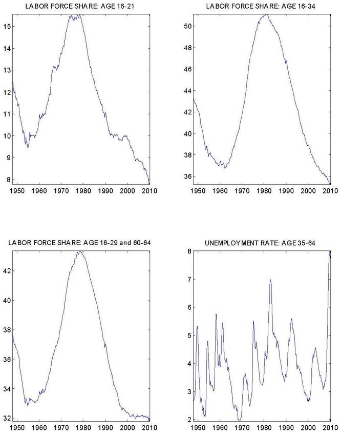
Unemployment and Productivity in the Long
        Run: the Role of Macroeconomic Volatility                                                            1

                    Pierpaolo Benigno (*), Luca Antonio Ricci (*), Paolo Surico (**)

Abstract

    We propose a theory of low-frequency movements in unemployment based on downward
real wage rigidities. The theory generates two main predictions: long-run unemployment
increases with (i) a fall in long-run productivity growth and (ii) a rise in the variance of
productivity growth. Evidence based on U.S. time series and on an international panel strongly
supports these predictions. The empirical specifications featuring the variance of productivity
growth can account for two U.S. episodes which a linear model based only on long-run
productivity growth cannot fully explain. These are the decline in long-run unemployment over
the 1980s and its rise during the late 2000s.

JEL Classification: E0, E20, E40.
Keywords: Unemployment, Productivity growth, Volatility.

(
 *) LUISS Guido Carli and EIEF IMF Research Department.
(**) London Business School and CEPR.
1
 We are grateful to Lawrence Ball, Olivier Blanchard, Renato Faccini, Giovanni Favara, Jordi Galì, Andrew Levin, Chris
Pissarides, Pau Rabanal, Valerie Ramey, David Romer, Julio Rotemberg, Giovanna Vallanti and to conference
participants at NBER Monetary Economics Meeting, the invited panel session on monetary policy of the European
Economic Association Congress in Glasgow and the Sveriges Riks-bank conference on "The Labor Market and the
Macroeconomy" for helpful discussions. Federica Romei has provided excellent research assistance. Pierpaolo Benigno
acknowledges financial support from an ERC Starting Independent Grant. The views in this paper are those of the
authors and do not necessarily refiect the views of the IMF, or IMF policy.

    1
CONTENTS

1          INTRODUCTION ............................................................................................................ 3
2          THE MODEL .................................................................................................................. 6
    2.1        FLEXIBLE WAGES .......................................................................................................... 9
    2.2        DEFINITION OF UNEMPLOYMENT RATE ............................................................................ 9
    2.3        STICKY REAL WAGES .................................................................................................... 10
    2.4        DOWNWARD REAL WAGE RIGIDITY ................................................................................. 15

3          EVIDENCE FOR THE UNITED STATES ..................................................................... 17
    3.1        MEASURING UNEMPLOYMENT AND PRODUCTIVITY TRENDS ............................................                             18
    3.2        THE FIT OF THE LINEAR MODEL ....................................................................................        20
    3.3        CONTROLLING FOR DEMOGRAPHICS .............................................................................              22
    3.4        THE FIT OF THE NONLINEAR MODEL ..............................................................................           24

4          INTERNATIONAL EVIDENCE ...................................................................................... 25
5          CONCLUSION ............................................................................................................. 28
REFERENCES .......................................................................................................................... 29
APPENDIX A ............................................................................................................................. 31
APPENDIX B ............................................................................................................................. 33
APPENDIX C ............................................................................................................................. 35
APPENDIX D ............................................................................................................................. 36
APPENDIX E ............................................................................................................................. 37
APPENDIX F ............................................................................................................................. 42

    2
1            INTRODUCTION

       This paper proposes a theory in which the low-frequency movements in unemployment are
                                                                                                            2
explained by the low-frequency movements and the volatility of productivity growth . On the one
hand, an increase in long-run productivity growth lowers long-run unemployment. On the other
hand, a fall in the variance of productivity growth leads to a fall in long-run unemployment even
when long-run productivity growth remains flat. The key mechanism that explains these
relationships rests on the assumption that real wages, or more broadly real marginal costs,
adjust more easily upward than downward.
    A recent literature has highlighted the importance of real wage rigidities to explain labor-
market dynamics at business cycle frequencies. Shimer (2005), Hall (2005), Gertler and Trigari
(2009) and Blanchard and Gali (2010) show that real wage rigidities are important to account for
a number of stylized facts including the high volatility of employment and vacancies as well as
                                          3
the low volatility of real wages. This paper complements these studies by showing that real
rigidities can also account for unemployment dynamics at low frequencies and therefore it offers
a rationale for the empirical relationship between long-run unemployment, long-run productivity
growth and its variance.
     Our analysis is motivated by a number of empirical papers, including Bruno and Sachs
(1985), Phelps (1994), Blanchard et al. (1995), Blanchard and Wolfers (2000), Staiger, Stock,
and Watson (2001) and Pissarides and Vallanti (2007), which show time-series and cross-
country evidence in favor of a negative relationship between unemployment and productivity
growth at low frequencies. This literature is exemplified by Figure 1 which reports the trend in
unemployment, the trend in productivity growth and the variance of productivity growth for a
postwar sample of U.S. data. The time series plotted in the charts on the first row are obtained
computing averages and variances over five-year rolling windows. The charts on the second
row display similar objects obtained using the time-varying Vector AutoRegressive (VAR) model
described in Section 3.
     Two main features are evident. First, irrespective of the strategy used to look at the data
over the long-run, the charts on the first column of Figure 1 confirm the negative relationship
between long-run unemployment and long-run productivity growth documented in earlier
                  4
contributions. Second, a probably less known, yet very interesting, feature of the data is the
strong positive association between long-run unemployment and the variance of productivity
growth, which is uncovered in the charts on the second column. The Great Moderation in the
variance of productivity growth, for instance, coincides with a sharp fall in the unemployment
trend.
    The contribution of this paper is twofold. On the theoretical side, we develop a simple model

2
    The terms long-run, trend, mean and low-frequency are used interchangeably throughout the paper.
3
  Pissarides (2009) off ers a critical appraisal of wage stickiness as a driver of the cyclical volatility of unemployment in
search models.
4
 Results similar to Figure 1 are obtained using ten-year rolling windows, the Hodrick-Prescott and
Christiano-Fitzgerald filters.

     3
of the labor market based on the assumption of asymmetric real wage rigidities that can account
                                                                        5
for the two empirical findings summarized in Figure 1. On the empirical side, we evaluate
formally the predictions of the model by exploiting low-frequency movements in unemployment
and productivity growth either over time or across countries.

Figure 1     Long-run unemployment, long-run productivity growth and variance of productivity growth
              for the U.S., computed using ve-year rolling windows for the charts on the first row and
                         the time-varying VAR of section 3 for the charts on the second row

5
    The significance of downward real wage rigidity has been documented by a large number of empirical studies on
micro-data, which are difficult to summarize in a few lines. Prominent examples include Dickens et al. (2008), Du Caju et
al. (2009), Fagan and Messina (2009), Holden and Wulfsberg (2009) for the industrialized world and Calvo et al. (2006)
for emerging markets.

     4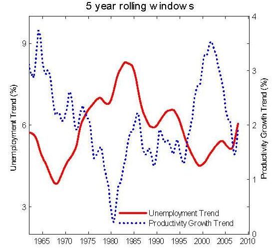
In our model, wage setters face convex costs for adjusting real wages which can be either
symmetric or asymmetric up to a limiting point that nests complete downward infiexibility.
Asymmetric real-wage rigidities have two key implications. First, for a given volatility of
productivity growth, a slowdown in long-run productivity growth generates a significant rise in
long-run unemployment. This is the case because too high real wages make it more likely that
real revenues will fall relative to costs, thereby forcing firms to reduce labor demand in order to
protect profits. With symmetric rigidities, this trade-off is weaker. Second, for a given long-run
productivity growth, a higher volatility raises the probability of an adverse shock and then leads
to higher long-run unemployment. Conversely, even when the trend in productivity growth is
low, a decline in its volatility reduces these risks and causes the unemployment trend to fall.
     We present evidence consistent with the predictions of the theoretical model. Time series
for the long-run mean and the variance of U.S. unemployment and productivity growth are
obtained using an estimated VAR with drifting coefficients and stochastic volatility á la Cogley
and Sargent (2005), and Primiceri (2005). Panel regressions are obtained using averages and
variances over ten-year windows within a dataset of industrialized and emerging economies.
     Our main results can be summarized as follows. First, the long-run mean and the variance
of productivity growth are significant determinants of the long-run mean of U.S. unemployment.
This is true even when we control for changes in the demographic composition of the labor
force. Second, the empirical specifications that include a measure of productivity growth
volatility (either linearly or non-linearly) are associated with a significant improvement in the
goodness of fit relative to a linear specification in longrun productivity growth only. This is
exemplified by two episodes that cannot be fully explained by movements of productivity growth
at low frequencies: the fall in long-run unemployment over the 1980s and its rise during the late
2000s. Third, the panel regressions reveal that variation over time is more important than
variation across countries for the mean and variance of productivity growth to account for
fiuctuations in the mean of unemployment.
     Few theoretical papers have studied the implications for the long-run relationship between
unemployment and productivity growth but, to the best of our knowledge, none has emphasized
the importance of time variation in macroeconomic volatility for the unemployment trend. In
traditional labor search models, the relationship between productivity and unemployment is
generally uncertain, as it depends mostly on the extent to which jobs can be upgraded or need
to be eliminated when new technology arises (Mortensen and Pissarides, 1998). If firms cannot
embody the new technology into existing jobs, higher productivity would lead to job destruction
and higher unemployment (Aghion and Howitt, 1994). If productivity increases for all existing
jobs, demand for labor would increase and unemployment would decline (Pissarides, 2000,
Pissarides and Vallanti, 2007). In line with our assumption of real wage rigidities, Ball and
Mankiw (2002) suggest a possible rationale for a negative relationship between unemployment
and productivity “resting on the idea that wage aspirations‟adjust slowly to shifts in productivity
growth”, as “workers come to view the rate of real wage increase that they receive as normal
and fair and to expect it to continue”.
     Our work complements an important literature which has built the case for demographic
changes in labor force participation to explain low-frequency movements in unemployment (see
Shimer, 1998, and Francis and Ramey, 2009, among others). We show that the finding of a
significant role for the trend and the variance of productivity growth to account for the trend in

  5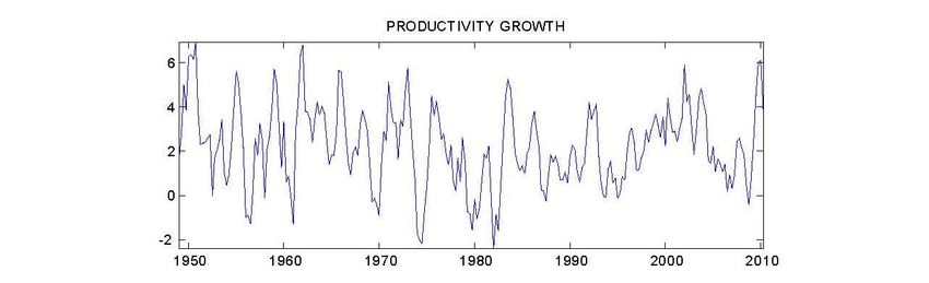
unemployment is robust to controlling for movements in the share of young workers in the labor
force as well as to using the measure of “genuine” unemployment that Shimer (1998) argues to
be unaffected by demographics infiuences.
     The paper is organized as follows. Section 2 presents the model and shows the mechanism
through which asymmetric real wage rigidity generates a long-run relationship between
unemployment, productivity growth, and its volatility. Section 3 confronts the predictions of the
model to the time series properties of U.S. data while Section 4 provides evidence for an
international panel of developed and developing economies. Section 5 concludes. The
appendices provide details of the theoretical and empirical models.
     The appendices provide details of the theoretical and empirical models.

2        THE MODEL

    We describe a closed-economy model in which there is a continuum of infinitely lived
households and firms (both in a [0,1] interval). Each household derives utility from the
consumption of a continuum of goods aggregated using a Dixit-Stiglitz consumption index, and
disutility from supplying one of the varieties of labor to firms in a monopolisticcompetitive
market. Each firm hires all varieties of labor to produce one of the continuum of consumption
goods and operates in a monopolistic-competitive market. The economy is subject to an
aggregate productivity shock. This is denoted by   At, whose logarithmic at is distributed as a
                                           2
Brownian motion with drift g and variance σ

                                                                                              (1)

where Bt denotes a standard Brownian motion with zero drift and unit variance.
    Household j has preferences over time given by

                                                                                              (2)

where the expectation operator   Et0(·) is defined by the shock processes (1) and ρ > 0 is the
rate of time preference. Current utility depends on the Dixit-Stiglitz consumption aggregate of
the continuum of goods produced by the firms operating in the economy

                                                                                 j
where θp > 0 is the elasticity of substitution among consumption goods and ct (i) is household
j’s consumption of the variety produced by firm i. An appropriate consumption-based price
index is defined as

    6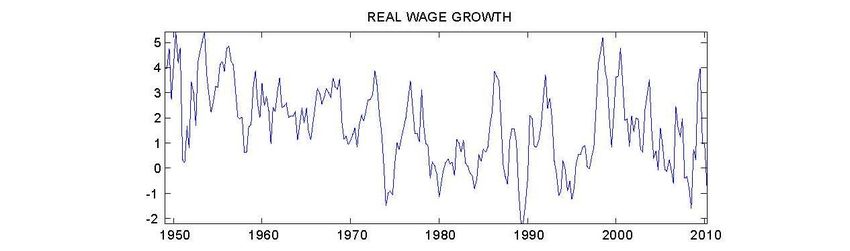
where pt(i) is the price of the single good i.
       The utility fiow is logarithmic in the consumption aggregate. In (2), labor disutility is
assumed to be isoelastic with respect to the labor supplied lt(j), with                        η ≥ 0 measuring the
                                                          6
inverse of the Frisch elasticity of labor supply. Household j’s intertemporal budget constraint is
given by

                                                                                                               (3)

where     Qt is the stochastic nominal discount factor in capital markets where claims to monetary
                                                                                           j
units are traded;      Wt(j) is the nominal wage for labor of variety j, and Πt is the profit income of
household j.
                                                                                                           j
       Starting with the consumption decisions, household                j chooses goods demand,{ct (i)}, to
maximize (2) under the intertemporal budget constraint (3), taking prices as given. The first-
order conditions for consumption choices imply

                                                                                                               (4)

                                                                                                               (5)

where the multiplier       ξ does not vary over time. The index j is omitted from the consumption‟s
first-order conditions, because we are assuming perfect consumption risk-sharing through a set
of state-contingent claims to monetary units.
     Before we turn to the labor supply decision, we analyze the firms‟problem. We assume that
the labor used to produce each good             i is a CES aggregate, L(i), of the continuum of individual
types of labor j defined by

with an elasticity of substitution θw > 1. Here li,t(j) is the demand of firm i for labor of type j.
Given that each differentiated type of labor is supplied in a monopolistic-competitive market, the
demand for labor of type j on the part of a wage-taking firm of type i is given by

                                                                                                               (6)

where Wt is the Dixit-Stiglitz aggregate wage index

                                                                                                               (7)

6
    These preferences are consistent with a balanced-growth path as we assume a drift in technology.

     7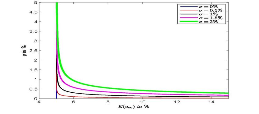
whereas the aggregate demand of labor of type j is given by

                                                                                                                     (8)

and the aggregate labor Lt is defined as

       We assume a common linear technology for the production of all goods

                                                                                                                     (9)

for a parameter        α with 0 < α < 1 measuring decreasing return to scale. Profits of the generic
firm i, Πt(i), are given by

       In a monopolistic-competitive market, given (5), each firm faces the demand

where total output is equal in equilibrium to aggregate consumption                     (Yt = Ct). We assume that
firms can freely adjust their prices. Standard optimality conditions under monopolistic
competition imply that all firms set the same price given by

                                                                                                                    (10)

where      µp ≡ θp/[(θp - 1)α] > 1 denotes the mark-up of prices over marginal costs.7 An
implication of (10) is that labor income is a constant fraction of total income

                                                                                                                    (11)
       Using the production function (9) into (11), aggregate demand of labor

depends negatively on the real wage and positively on productivity. Demand of labor is critical
to understand the main intuition behind our results. When productivity falls and real wage
remains too high, firms have to cut on labor to protect their profits.
       In what follows, we define           wt(j) = Wt(j)/Pt as the real wage for worker of type j and
wt = Wt /Pt as the aggregate real wage.8 The choice of real wages is modelled in a similar way

7
    See the Appendix for the derivation of equation (10).
8
    Notice that equation (11) holds because of the assumption of fiexible prices which is necessary for analytical
tractability.

     8
to the monopoly-union model of Dunlop (1944). Given firms‟demand (8), a household of type j
(or a union) chooses real wages in a monopolistic-competitive market to maximize (2) under the
intertemporal budget constraint (3) taking as given prices {Qt} and the other relevant aggregate
variables. An equivalent formulation of this problem is the maximization of the following
objective
(13)
∞
by choosing {wt(j)} , where
Households would then supply as much labor as demanded by firms in (8) at the chosen
real wages. In deriving π(·) we have used (4), (8) and (11).
2.1 Flexible wages
We first analyze the case in which wages are set without any friction, so that they can be
moved freely. With fiexible wages, maximization of (13) corresponds to per-period maximization
and implies the following optimality condition
(14)
where πwj(·) is the derivative of π(·) with respect to the first argument. Since equation (14)
f f
holds for each j, there is a unique equilibrium where wt(j) = wt = wt and in which wt denotes
the equilibrium level of real wages under fiexible wages. Equation (14) defines the equilibrium
level of labor under fiexible wages, which is a constant given by
where the wage mark-up is defined by µw ≡ θw/(θw - 1). Real wages are proportional to the
aggregate productivity shock
(15)
2.2 Definition of unemployment rate
Following Galì (2010), we define the unemployment rate as the difference between the
“notional” amount of labor that workers would be willing to supply in a competitive and
frictionless market at the current real wage and the amount of labor currently employed. Given
s
our preference specifications, “notional” labor supply, Lt , is defined as the amount of labor that
equates the marginal rate of substitution between labor and (current) consumption to the current
real wage
(16)
9s
Accordingly, the unemployment rate ut is given by ut = ln Lt - ln Lt. Combining (16) with
(11) and using Yt = Ct we can write
(17)
where uf denotes the unemployment rate in the fiexible-wage model given by uf = ln µw/η and
where the employment gap xt, equal to the output gap, is defined as the log difference between
actual labor and the fiexible-wage level
(18)
With fiexible wages, unions set too high real wages and at these real wages workers would
be willing to supply more labor than currently demanded by firms. Unemployment is given by uf
and indeed captures the unions‟monopoly power. With real wage rigidities, unemployment
depends also on the output gap and can vary over time inversely proportional to the variation of
the output gap. This second component will be the most relevant in our model to explain the
dynamics of unemployment at low frequencies.
2.3 Sticky real wages
In this section, we investigate a general model in which real wages are allowed to adjust
either upward or downward but with some cost. In particular, we allow for both symmetric and
asymmetric adjustment costs through a linex function of the form
for some parameters χ, λ, where we have defined the rate of real wage changes as
πR,t(j)dt ≡ dwt(j)/wt(j). In particular χ is a measure of the costs of adjustment, while λ
9
measures the asymmetries in the cost function. When λ → 0, we retrieve the standard
symmetric quadratic cost function
while when λ < 0 it is more costly to adjust real wages downward than upward and viceversa
for λ > 0. When λ goes to minus infinity, we nest the case in which real wages are infiexible
downward and fully fiexible upward. In the next section, we discuss this case more extensively
as it allows us to derive a closed form solution for the long-run mean of unemployment.
9
Varian (1974) has first introduced this specification. Kim and Murcia (2009) have recently used it to model asymmetric
nominal wage rigidities.
10In this setting, we assume that wage setters maximize (13) taking into account the present
10
discounted value of the costs of changing real wages
(19)
The value function associated with the objective function (19) can be written as
(20)
where
(21)
and in which we have used the results that (dwt(j))2 = (dwt)2 = dwt(j)dAt = dwtdAt = 0 and
defined g' ≡ g + (1/2)σ .
2 11
Using the expression for the value function given by (20) and (21), we obtain the optimal
value of πR,t(j) as implicitly defined by the following condition
(22)
where
(23)
In the symmetric case, i.e. when λ → 0, the rate of real wage changes is proportional to its
marginal cost
Using (20), (21) and (22), we show, in Appendix D, that the marginal costs of changing real
wages follow a stochastic differential equations of the form
(24)
and therefore
(25)
Under a quadratic cost function, we can simplify equation (24) to
10
With similar tools, Abel and Eberly (1994) have analyzed costly investment decisions.
11
The fact that dwt has the same properties of dwt(j) follows from the symmetry of the equilibrium.
11which is the continuos-time non-linear version of the Rotemberg‟s (1982) cost of adjustment
model where the stickiness is applied to real wages rather than to nominal wages and where we
have defined k ≡ (θw - 1)/(µpχ2).
Using the definition of the employment gap (18), equation (12) implies that
(26)
and therefore a diffusion process for xt of the form
(27)
which can be used to derive the long-run distribution and in particular the long-run mean of the
employment gap, x. To this end, we need to solve for the unknown functional πR(xt). By defining
p(xt) ≡ hπ(πR(xt))/χ2, the optimality condition (23) implies
(28)
In particular, using Ito‟s Lemma in equation (24) and the difusion process (27), we obtain
that the functional p(xt) satisfies the following differential equation
(29)
Notice again that with quadratic adjustment costs πR(xt) = p(xt). We use (28) and (29) to
solve for the functional πR(xt) and p(xt) and then (27) to solve for the long-run distribution of xt,
if it exists.
2.3.1 The productivity growth-unemployment trade-off
The differential equation (29) is solvable using approximation methods. In particular, an
educated guess would be to approximate the solution p(xt) with a finite-order polynomial.12 An
interesting case, which can be helpful to discuss first, is that of a first-order polynomial.
Consider the symmetric quadratic adjustment cost model, with λ → 0, and (1+η)xt consider
(1+η)xt (1+η)xt
small deviations of xt from zero. In particular, approximate the term e in (29) as e ≈
1+ (1+ η)xt. In this case, the solution for p(xt), which is equal to πR(xt), is linear and of the form
p(xt) = πR(xt) = a0 + a1xt where a1 is the positive root of the following quadratic equation
and
12
This is an educated guess since both the exponential in (29) and the logarithmic in (28) can be represented with
infinite-order polynomials, althought the latter only when |p(xt)| < 1.
12From the stochastic differential equation (27), it can be seen that the employment gap, xt,
follows an Ornstein-Uhlenbeck process which in the long run converges to a normal distribution
with mean given by
where x∞ denotes the long-run level of the employment gap. The above equation displays a
positive relationship between the employment gap and productivity growth and therefore a
negative linear relationship between unemployment and productivity growth
where we have used (17). Notice that at lower levels of real-wage stickiness (lower χ) the link
between unemployment and productivity growth is weakened and unemployment becomes
close to the frictional level. Furthermore, in this linear solution, there is no relationship between
unemployment and the volatility of productivity growth.
In order to find a role for volatility, we need to take at least a second-order polynomial
approximation forp(xt) and πR(xt).13 However, as shown in Figure 2, when we assume a
symmetric adjustment-cost function, λ → 0, we find that the trade-off between unemployment
and productivity growth is negligible and the curve is almost vertical. Moreover the variance has
14
a small role in accounting for significant shifts in such a trade-off.
Figure 2 Model with symmetric real-wage rigidities: long-run relationships between the mean of
unemployment, E(u∞), and the mean of productivity growth, g, for different values of the
standard deviation of productivity growth, σ. All variables in % and at annual rates.
13
The approximations are accurate as long as xt, p(xt) and πR(xt) remain appropriately bounded within the unit circle.
In particular, a larger λ in absolute value requires stricter bounds for xt.
14
In the Figure, we use the following calibration: η = 2.5, ρ = 0.04, α = 0.66,θ = 6, µp= 1.15, µf = 0.05, χ = 1.77. In
particular, within a Calvo model the assumption on χ would translate into an average duration of contracts on real
wages equal to one year and a half. Note that, as shown in Figure 1, the VAR estimates of the variance of productivity
growth range between 0.0001 and 0.0005, implying standard deviations in the range 1% to 2.3 per cent.
13A stronger trade-off and a more important role for volatility emerge when there are
asymmetries in real wage rigidities, as shown in Figure 3 where we let the parameter λ take
negative values. As λ decreases the trade-off becomes more pronounced in a way that it also
depends on the level of productivity growth. Moreover, the lower λ the higher the impact of
volatility on unemployment. This channel is larger the closer the trend in productivity growth is to
zero.
Figure 3 Model with asymmetric real-wage rigidities: long-run relationships between the mean of
unemployment, E(u∞), and the mean of productivity growth, g, for different values of the
standard deviation of productivity growth, σ, and different levels of asymmetries, λ.
All variables in % and at annual rates.
When there are asymmetric rigidities on the downward side, lower levels of productivity
growth are associated with higher unemployment because bad productivity shocks are more
likely to be absorbed by lower employment demand on the side of firms, as in (12). Firms cut on
labor to protect their profits since real wages cannot fall much. At these too high real wages
workers would like to supply more labor than what firms demand. When the volatility of
productivity growth is high, these bad draws on productivity are even more likely requiring a
larger adjustment on labor.
The mechanisms underlined by our model would be absent in a simple framework of
symmetric real wage rigidities unless there is a substantial and persistent misalignment
between real wages growth and productivity growth. Not only would a model with symmetric
real rigidities imply a weak relationship between productivity growth and unemployment but also
no role for the volatility of productivity growth in explaining unemployment.
In the next section, we discuss more extensively the results in the limiting case of complete
downward real wage infiexibility.
2.4 Downward real wage rigidity
In this section, we assume that real wages are completely rigid on the downward side and
fiexible on the upward side. This model can be solved in closed-form and its derivation of its
1415
solution is helpful to illustrate the infiuence of volatility on unemployment. With complete
downward wage infiexibility, the wage setters maximize (13) under
(30)
with wt0 > 0. In other words, agents choosea non-decreasing positive real wage path to
maximize (13). In appendix E, we show that this optimization problem leads to a simple decision
rule. Wage setters compare their past choice on real wages to a current desired real wage.
Whenever the past real wage is higher than the desired one, they are constrained by the past
decisions and cannot move their real wage. Otherwise, whenever the current desired real wage
d
is higher than the past real wage, they adjust upward to that desired real wage, wt , which is a
fraction of the fiexible-wage level and given by
(31)
where c(·) is a non-negative function of the model parameters:
(32)
and γ(·) is the following non-negative function
which is derived in Appendix E.
Agents‟ optimizing behavior in the presence of exogenous downward real wage rigidities
implies an endogenous tendency for limiting the upward revisions in real wages. When wages
d
adjust upward, they adjust to the desired level wt , which is always below the fiexible-wage level
by a factor c(·). Indeed, optimizing wage setters choose an adjustment rule that tries to
minimize the inefficiencies of downward real wage infiexibility. Wage setters are worried to get
locked with an excessively high real wage were future unfavorable shocks require a real wage
decline (as downward real wage rigidities would imply a fall in employment). As a consequence,
optimizing agents refrain from excessive real wage increases when favorable shocks require
upward adjustment, pushing current employment above the fiexible-case level.
The above optimizing decision rule nests also a myopic rule in which agents do not take
into account the consequences of the current real wage choice for future decisions and simply
adjust real wages to a fiexible-wage level whenever this level is above their previous choice. In
f
this case wt = wt , whenever dwt > 0. This myopic rule, which will be of particular interest for
the empirical section that follows, corresponds to the limiting case in which agents do not
discount the future at all, i.e. when ρ → ∞ implying c → 1.
15
Benigno and Ricci (2010) study the implications of a model with downward nominal wage rigidities.
152.4.1 The productivity growth-unemployment trade-off
We can now solve for the equilibrium level of employment and characterize the productivity-
unemployment trade-off in the presence of downward real wage rigidities. Since we have shown
f
that wt ≥ c(·)1−α wt equation (26) implies that -∞ ≤ xt ≤ -ln c(·). The existence of downward
real wage rigidities endogenously adds an upward barrier on the employment gap. Since at
follows a Brownian motion with drift g and standard deviation σ, also xt is going to follow a
2
Brownian motion with mean g/(1 - α) and variance (σ /(1 - α)) but with a regulating barrier at
-ln c(·). The probability distribution function for such process can be computed at each point in
16
time. We are interested in studying whether this probability distribution converges to an
equilibrium distribution when t → ∞, in order to characterize the long-run probability distribution
for employment, and thus unemployment. Standard results assure that this is the case when the
drift of the Brownian motion of xt is positive, which requires g > 0. In this case, it can be shown
that the long-run cumulative distribution of xt, denoted with P(·), is given by
for 0 ≤ z ≤ -ln c(·) where x∞ denotes the long-run equilibrium level of the employment gap. We
can compute the long-run mean of the employment gap,
(33)
and therefore the long-run mean of unemployment
(34)
In this model the average growth rate of real wages converges in the long run to the
17
productivity trend, g for any positive g. In the presence of downward real wage rigidities, we
find a strong negative relationship between the unemployment rate and the rate of productivity
growth, which is shifted by the volatility of productivity. The shift is quantitatively important as
shown in Figure 4. For given growth of productivity, a higher volatility implies a higher
unemployment rate. For given volatility, a lower productivity growth implies a higher
unemployment rate. Notice that under the myopic adjustment rule, in which ρ → ∞, the mean of
unemployment rate is simply given by
(35)
as the function c(·) in (34) is now equal to 1. Indeed, a value of c(·) below one is capturing the
benefits in terms of lower unemployment due to the intertemporal optimizing behavior of wage
setters who are taking into account the future consequences of their current real wage choices
16
See Cox and Miller (1990, pp. 223-225) for a detailed derivation.
17
This is an appealing feature of the limiting case in contrast with the model of symmetric rigidities .
16and therefore set lower real wages when adjusting upward. Absent this channel, unemployment
would simply refiect the structural level of unemployment, u f, and the costs of the downward
real wage rigidity constraint given by the ratio between the variance and the mean of
productivity growth. The relevance of this ratio to explain long-run unemployment will be
investigated in the empirical analysis below.
Figure 4 Model with downward real-wage rigidities: long-run relationships between the mean of
unemployment, E(u∞), and the mean of productivity growth, g, for different values of
the standard deviation of productivity growth, σ. All variables in % and at annual rates.
3 EVIDENCE FOR THE UNITED STATES
A key prediction of the theoretical model is that the variance of productivity growth has
explanatory power for the mean of the unemployment rate over and above the mean of
productivity growth. There are two ways we can take this prediction to the data. First, focusing
on a single country, we can construct time-varying measures of mean and volatility, and then
ask whether periods of higher variance in productivity growth are associated with a higher mean
of unemployment, for a given mean of productivity growth. Second, we can investigate this
relationship within a panel of countries. This section describes the strategy and the results for
the first avenue. Section 4 presents evidence based on the second avenue.
As for exploiting the time variation within a single country, the U.S. Great Moderation
appears a natural candidate for assessing the empirical merits of our theory. During the first half
of the 1980s, the volatility of several measures of real activity, including real GDP growth,
residential investment and unemployment fell sharply in the U.S.. To the extent that productivity
growth also showed a pronounced decline in volatility, our model predicts that this should have
been accompanied by a pronounced fall in the mean of unemployment. Figure 1 provides prima
facie evidence in support of this prediction. In this section, we first spell out the way the
estimates in Figures 1 have been constructed and we then use the time-varying measures of
mean and volatility for productivity growth to assess the ability of the model to account for the
low-frequency variation in the unemployment rate.
173.1 Measuring unemployment and productivity trends
The econometric literature offers several ways to model time-variation in the variance of the
stochastic disturbances as well as in the autoregressive coeffi cients of stochastic processes.
Some of the best-known examples in macroeconomics include models of AutoRegressive
Conditional Heteroskedasticity (ARCH), Regime-Switching volatility models (RS) and Vector
AutoRegressions with stochastic volatility (VAR). It is worth emphasizing that our theoretical
model has predictions for the rate of unemployment in the long-run. The focus on the long-run
makes the ARCH specification less attractive than the RS and the VAR. Furthermore, the notion
of real rigidities in the labor market hinges upon the presumption that changes in productivity
diffuse gradually, rather than abruptly, to the rest of the economy, thereby making the RS model
less attractive than the time-varying VAR for our purposes.
Following the literature pioneered by Cogley and Sargent (2001 and 2005), and followed
among others by Primiceri (2005) and Sargent and Surico (2011), we model the evolution of
productivity growth, gt, real wage growth, Δwt, and the rate of unemployment, ut, using a VAR
with drifting coeffi cients and stochastic volatility. The drifting coefficients enable us to construct
a time-varying measure for the mean of the endogenous variables. Both the drifting coeffi cients
and the stochastic volatility allow us to construct a time-varying measure of volatility.
The statistical model is a VAR(p) of the following form:
(36)
where Xt collects the first p lags of Yt , θt is a matrix of time-varying parameters, et are reduced-
form errors, Yt is defined as Yt ≡ [gt, Δwt,ut]' , and ρ is set equal to 2. The parameters of the
error covariance matrix, Var(et) ≡ Ωt, are assumed to evolve as geometric random walks while
the parameters of the matrix of autoregressive coefficients are assumed to evolve as random
walks.
The time-series for long-run unemployment and long-run productivity growth are computed
as local-to-date t approximations to the mean of the endogenous variables of the VAR,
evaluated at the posterior mean E(θt|T). Let us rewrite equation (36) in companion form:
where zt contains current and lagged values ofYt, Ct|T is the vector of intercepts, Dt|T is the
vector of stacked time-varying parameters and ςt is a conformable vector containing et and
zeros. Following Cogley and Sargent (2005), the long-run mean for the vector zt can then be
computed as:
(37)
where, given the order of the variables in the VAR, the first and third elements of correspond
to the mean of productivity growth, and the mean of unemployment, at time t.
The time-series for the unconditional variance of the variables in the VAR can be estimated
using the integral of the spectral density over all frequencies, , where ft|T is defined
as:
(38)
18The element (1,1) of the matrix ft|T(ω) represents the unconditional variance of productivity
growth, , at time t. Details of the model specification and estimation method are provided in
Appendix B.
The data were collected in September 2010 from the Fred database available at the Federal
Reserve bank of St. Louis. Productivity is the non-farm business sector output per hour of all
persons (acronym „OPHNFB‟), wage is the non-farm business sector real compensation per
hour (acronym „COMPRNFB‟), and unemployment is the rate of civilian unemployment for
18
persons with 16 years of age or older (acronym „UNRATE‟). All variables are seasonally
adjusted at the source. As we are not interested to explain quarter on quarter changes, we
compute annual growth rates for productivity and real wage to smooth out the high frequency
components in the data. Growth rates are approximated by log differences. Results are robust
to using quarterly changes. To calibrate the priors for the VAR coeffi cients, we use a training
sample of thirteen years, from 1949Q1-1961Q4. The results hereafter, then, refer to the period
1962Q1 to 2010Q2.
We can therefore compute the estimates of long run unemployment ( ), long run
productivity ( ), and the variance of productivity ( ) from the estimates of the VAR (36)
together with the formulas (37) and (38). These series are shown in Figure 1.
3.2 The fit of the linear model
This section assesses empirically the main predictions of the model: the mean of unem-
ployment depends negatively from the mean of productivity growth and positively from the
variance of productivity growth. More formally, we can write:
where the vector ϑ ≡ (η, ρ, α, λ, uf ) contains the relevant parameters of the model and f(·) is a
generic non-linear function which in the limiting case of downward real wage infiexibility
corresponds to (34).
A natural benchmark of comparison for this exercise is the linear specification employed in
earlier contributions (see for instance Pissarides and Vallanti, 2007), which relates long-run
unemployment to long-run productivity growth:
(39)
where a and b are parameters and εt is a well-behaved stochastic disturbance. Using the
estimates of the VAR derived in the previous Section, we obtain the following OLS estimates for
equation (39):
(40)
where standard errors are reported in parentheses. The R2 of the regression is 0.77. The
18
To make our empirical results comparable with earlier contributions (see for instance Staiger, Stock and Watson,
2001), we measure productivity as the ratio of output to total hours in the non-farm business sector, Y/L. This measure
is computed and released by the Bureau of Labour Statistics. In our model, productivity is defined as Y/Lα and the first
difference of its logarithm is denoted by g. It should be noted, however, that assuming a standard labour to capital ratio
of 2/3 the correlation between g and the first difference of the logarithm of Y/L is 0.91 over our sample period.
19estimates of this simple model show that there is a tight negative relationship between
productivity growth and unemployment in the long-run. In particular, a 1% fall in longrun
productivity growth corresponds to an increase in long-run unemployment of 2.24 percentage
points. Alternatively, an increase of one standard deviation (0.002) in longrun productivity
growth would lower long-run unemployment by 0.47 percentage points.
Figure 5 confronts long-run unemployment, depicted as red continuous line, with the fitted
values from equation (40), depicted as blue dotted line. The linear model does a good job in
Figure 5 Trend in the unemployment rate implied by the estimates of the time-varying VAR (36)
using formula (37), and fitted values of the Linear Model of equation (40) and of the
Linear Model with Variance of equation (41). Percent rates.
tracking qualitatively the movements in the unemployment rate. However, a closer inspection of
the figure reveals that neither the decline in trend unemployment between 1984 and 1992 nor
the rise since the late 1990s can be adequately explained by the linear model, whose fit seems
particularly inadequate to explain the developments in long-run unemployment since 2007.
The theoretical model of section 2 suggests two departures from the linear specification
(39). First, it highlights the relevance of the variance of productivity growth. Consistent with
Figure 1, movements in the variance of productivity growth coincide with movements in long-run
unemployment, especially during the periods where the mean of productivity growth was fiat.
Second, under the limiting case of downward real wage infiexibility, the model allows us to
derive a nonlinear relationship between unemployment and productivity growth in closed form.
To appreciate the relative importance of these modifications, we proceed in two steps. First we
augment the linear specification in (39) with a vari-ance term. Then, we estimate the
relationship between unemployment and productivity growth nonlinearly.
More specifically, we estimate the following linear specification in both the mean and the
variance of productivity growth:
(41)
20The variance term is highly significant and the R2 is now 0.95, a significant increase relative
to the estimates in (40) which are based on a linear specification in long-run productivity growth
19
only. The improvement is evident from Figure 5. The fitted values from equation (41) track
unemployment trend far better than the linear model (40), and in particular they allow the model
to account fully for the decline in long-run unemployment of the 1980 and the rise of the late
2000s. The coefficient on the productivity mean is somewhat lower than in the bivariate case.
The effect of the variance is also economically significant: an increase of one standard
deviation (0.00005) would imply a rise in long-run unemployment of about 0.25 percent. The
estimates in Figure 1 reveal that the variance of productivity growth declined from 0.0003 to
about 0.0002 during the first half of the 1980s when long-run unemployment fell from about
6.5% to 5.5%. Together with the estimates in (41), this implies that the decline in the variance of
productivity growth can account for about 50% of the fall in long-run unemployment during this
episode. Between 2000 and 2009, the variance of productivity growth has increased from
0.00024 to 0.00038 against the backdrop of a rise in long-run unemployment from 5% to 6%.
These numbers imply a 70% contribution of the variance of productivity growth to long-run
unemployment during the 2000s.
3.3 Controlling for demographics
An important strand of the literature has convincingly argued that changes in the
demographic composition of the labour force affects the low-frequency movements in
unemployment (Shimer, 1998), the low-frequency movements in productivity (Francis and
Ramey, 2009) and the variance of real output growth (Jaimovich and Siu, 2009).
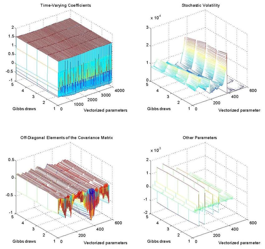
In this section, we want to assess the extent to which the estimates of the linear models
above may vary once we control for demographics. To this end, we construct time series for the
share of workers in the labor force with age (i) between 16 and 21 (as in Francis and Ramey,
2009), (ii) between 16 and 34 (as in Shimer, 1998), and (i) the sum of the shares of workers in
the 16-29 and the 60-64 windows of age (as in Jaimovich and Siu, 2009). Furthermore, we run
a regression of the unemployment rate on a constant and the unemployment rate of workers in
prime age (defined as those between 35 and 64 years), and then use the fitted values from this
regression in place of the unemployment rate in the VAR to construct the trend of what Shimer
(1998) refers to as a measure of genuine unemployment which is not affected by
20
demographics.
The labor force series were collected in September 2010 from the Bureau of Labor
Statistics using data gathered in the Current Population Survey. These data can also be used to
compute the unemployment rate for prime-age workers. The series used in this section are
reported in Appendix A. The results of these sensitivity analyses are collected in Table 1, which
presents estimates for the linear model using the trend of productivity growth and the measures
of labor force share in columns (1) to (3), and then adding the variance of productivity growth in
19
Similar results are obtained using averages and variances of unemployment and productivity growth computed over
either five-or ten-year rolling windows.
20
The estimates of this regression are: 0.0075 (.0014) for the intercept and 1.2716 (.0340) for the slope. Standard
2
errors in parenthesis. R = 0.851. Sample: 1948Q1:2010Q2.
2122
Table 1 Controlling for demographicscolumns (5) to (7). The estimates for the specifications using Shimer‟s measure of genuine
unemployment are displayed in columns (4) and (8), without and with the variance of
productivity growth respectively.
Two main results emerge from Table 1. First, controlling for demographics does not
overturn our finding of a significant role for both the long-run mean and the variance of
productivity growth to explain low-frequency movements in unemployment. In particular, the
estimated coefficient on in columns (5) to (8) is never statistically different from the estimates
in (41), which omits any demographic measures. Similar results are obtained for the estimated
coefficient on although in column (4) this is statistically lower than the estimates in (40).
Second, in line with Shimer (1998), Francis and Ramey (2009) and Jaimovich and Siu (2009),
the composition of the labor force has a significant infiuence on the low-frequency movements
in unemployment, although its statistical and economic significance appear muted once the
variance of productivity growth is added as additional regressor in the columns (5) to (7). The
finding of an important role for the variance of productivity growth is robust to using Shimer‟s
measure of genuine unemployment in column (8), although the coefficient on the productivity
growth trend is statistically smaller than in (41).
In summary, we conclude that the long-run mean and the variance of productivity growth
are significant determinants of U.S. long-run unemployment over and above changes in the
demographic composition of the labor force in the post-WWII period.
3.4 The fit of the nonlinear model
The results above point toward a significant role for asymmetries in real wage rigidities. To
investigate this channel further, we estimate the non-linear equation implied by the model under
the limiting case of complete downward real wage rigidities:
(42)
Unfortunately, the parameters α and η are not separately identified. Nevertheless, we can
still estimate a reduced-form version of (42), which we refer to as the “unrestricted model”.
The estimates of the unrestricted model yield so high estimates for ρ as to imply values of
the function c(·) very close to one, which correspond to the case of myopic agents. We
therefore estimate also a simplified version of the theoretical model in (42) where we impose
c = 1 prior to estimation:
(43)
The simplified version (43), which is linear in the variance-to-mean ratio of productivity
growth, is referred to as the „restricted model‟.
The fitted values associated with the non-linear unrestricted model and with the variance-to-
mean restricted model are presented in Figure 6. Both specifications track long-run
unemployment remarkably well and they clearly outperform the linear specification of Figure 5
which is based on long-run productivity growth only. In particular, the specifications in (42) and
(43) capture well the fall in long-run unemployment during the 1984-1992 period and its
increase during the (late) 2000s.
23Figure 6 Trend in the unemployment rate implied by the estimates of the time-varying VAR (36)
using formula (37), and fitted values for the Non-linear Unrestricted model of equation (42)
and the Variance-to-Mean-Ratio model of equation (43). Percent rates.
The non-linear model has a R2 of 0.92 and a point estimate (standard error) for the fiexible-
wage unemployment rate, µf, of 3.88% (0.29). The restriction implied by the variance-to-mean
2
ratio implies only a modest deterioration in the goodness of fit with a R of 0.90 and a coefficient
µf of 3.41% (0.05). This suggests that the simplified expression (43) provides a reasonable
approximation to the unrestricted specification (42). Notice again that in the simplified model
(43) with myopic agents, downward real wage rigidities play a crucial role through the infiuence
of the variance-to-mean ratio of productivity growth in affecting unemployment in the long-run.
In summary, versions of the theoretical model that feature strong asymmetries in real
rigidities appear to account for the low-frequency movements in the U.S. unemployment rate
which a model with symmetric real rigidity has hard time to explain. Similar results, available
upon request, are obtained using Shimer‟s measure of genuine unemployment, which controls
for demographic changes.
244 INTERNATIONAL EVIDENCE
In this section, we explore the empirical implications of the model in Section 2 within a
panel of international data. In particular, we are interested in whether the variance of
productivity growth has predictive power for the mean of unemployment across different
countries over a sufficiently long period of time. Our international dataset is an unbalanced
panel of quarterly observations for developed and developing economies over the post-WWII
21
period.
For each country i, we compute over a window of ten years:
1) the mean of unemployment, ;
2) the mean of productivity growth, ;
3) the variance of productivity growth, ;
4) the ratio between the variance of productivity growth and the mean itof productivity
growth, V-to-M ratioit.
Unemployment is taken from various data sources (World Development Indicators, IFS,
WEO, OECD, and Datastream, via splicing in the respective order); the sample spans the years
between 1960 and 2008. For productivity, we use real GDP per worker where real GDP is taken
from employment World Development Indicators, IFS, and WEO (via splicing in the respective
order) and employment is taken from the same sources as unemployment. Prior to estimation,
we drop observations for which there are less than eight periods in a ten-year window. The
estimates are displayed in Table 2 and each column refers to a different specification and
estimation method. The estimates in the first eight columns are based on the Fixed-effect
Estimator (FE) with time dummies included only in the columns (5) to (8). The last two columns
refer to the Between Estimator (BE) and will allow us to assess the extent to which cross-
country variation in the mean of unemployment is due to crosscountry variation in the mean and
variance of productivity growth. In all specifications, standard errors are adjusted for
heteroskedasticity. In the FE columns, standard errors are also adjusted for intra-group
correlation. In line with the theory, the coefficient on average productivity growth is negative and
the coefficient on the variance of productivity growth is positive. While the latter is always
significant, the former is significant only in the specifications that do not include time dummies.
A possible interpretation of this result is that the countries in our panel share a common trend in
productivity growth which absorbs the negative correlation with national unemployment. The
coefficients are somewhat lower than those estimated in the previous section, in part refiecting
higher standard deviations for all variables in this international sample. Indeed, the coefficient in
column 3 indicates that the effect of a one standard deviation increase in productivity growth
(about 0.02) is to lower average unemployment by a full percentage point.
The significance of the variance of productivity growth is strongly supported. The estimated
coefficient on the variance to mean ratio is positive and statistically different from zero in both
specifications (4) and (8), and therefore it accords with the prediction of the model of section 2.
21
The countries are: Argentina, Australia, Austria, Belgium, Bulgaria, Canada, Chile, China,P.R.:Hong Kong, Czech
Republic, Denmark, Estonia, Finland, France, Germany, Greece, Hungary, Iceland, Ireland, Israel, Italy, Japan, Korea,
Latvia, Lithuania, Luxembourg, Malaysia, Malta, Morocco, Netherlands, New Zealand, Norway, Peru, Philippines,
Portugal, Russia, Slovak Republic, Slovenia, Spain, Sweden, Switzerland, Taiwan Prov.of China, Thailand, United
Kingdom, United States, Venezuela, Rep. Bol.
25You can also read