Statistical shape analysis of large datasets based on diffeomorphic iterative centroids - bioRxiv
←
→
Page content transcription
If your browser does not render page correctly, please read the page content below
bioRxiv preprint first posted online Jul. 6, 2018; doi: http://dx.doi.org/10.1101/363861. The copyright holder for this preprint
  (which was not peer-reviewed) is the author/funder, who has granted bioRxiv a license to display the preprint in perpetuity.
                                 It is made available under a CC-BY-ND 4.0 International license.

Statistical shape analysis of large datasets
based on diffeomorphic iterative centroids.
Claire Cury 1,2,3,4,∗ , Joan A. Glaunès 5 , Roberto Toro 6,7 , Marie Chupin 1,2,4 ,
Gunter Shumann 8 , Vincent Frouin 9 , Jean-Baptiste Poline 10 , Olivier
Colliot 1,2,4 , and the Imagen Consortium 11
1 Sorbonne Universités, Inserm, CNRS, Institut du cerveau et de la moelle épinière
(ICM), AP-HP - Hôpital Pitié-Salpêtrière, Boulevard de l´ hôpital, F-75013, Paris,
France
2 Inria Paris, Aramis project-team, 75013, Paris, France
3 Inria Rennes, VISAGES project-team, 35000, Rennes, France
4 Centre d´ Acquisition et de Traitement des Images (CATI), Paris and Saclay,
France
5 MAP5, Université Paris Descartes, Sorbonne Paris Cité, France
6 Human Genetics and Cognitive Functions, Institut Pasteur, Paris, France
7 CNRS URA 2182 “Genes, synapses and cognition”, Paris, France
8 MRC-Social Genetic and Developmental Psychiatry Centre, Institute of
Psychiatry, King’s College London, London, United Kingdom
9 Neurospin, Commissariat à l’Energie Atomique et aux Energies Alternatives,
Paris, France
10 Henry H. Wheeler Jr. Brain Imaging Center, University of California at Berkeley,
USA
11 http://www.imagen-europe.com

Correspondence*:
Claire Cury
claire.cury.pro@gmail.com

ABSTRACT
  In this paper, we propose an approach for template-based shape analysis of large datasets,
using diffeomorphic centroids as atlas shapes. Diffeomorphic centroid methods fit in the Large
Deformation Diffeomorphic Metric Mapping (LDDMM) framework and use kernel metrics on
currents to quantify surface dissimilarities. The statistical analysis is based on a Kernel Prin-
cipal Component Analysis (Kernel PCA) performed on the set of momentum vectors which
parametrize the deformations. We tested the approach on different datasets of hippocampal
shapes extracted from brain magnetic resonance imaging (MRI), compared three different cen-
troid methods and a variational template estimation. The largest dataset is composed of 1000
surfaces, and we are able to analyse this dataset in 26 hours using a diffeomorphic centroid. Our
experiments demonstrate that computing diffeomorphic centroids in place of standard variational
templates leads to similar shape analysis results and saves around 70% of computation time.
Furthermore, the approach is able to adequately capture the variability of hippocampal shapes
with a reasonable number of dimensions, and to predict anatomical features of the hippocampus
in healthy subjects.
Keywords: morphometry ; statistical shape analysis ; template ; diffeomorphisms ; MRI ; hippocampus ; IHI ; Imagen ; Centroids ;
LDDMM

1 INTRODUCTION
Statistical shape analysis methods are increasingly used in neuroscience and clinical research. Their
applications include the study of correlations between anatomical structures and genetic or cognitive
parameters, as well as the detection of alterations associated with neurological disorders. A current chal-
lenge for methodological research is to perform statistical analysis on large databases, which are needed
to improve the statistical power of neuroscience studies.

                                                                                                                                     1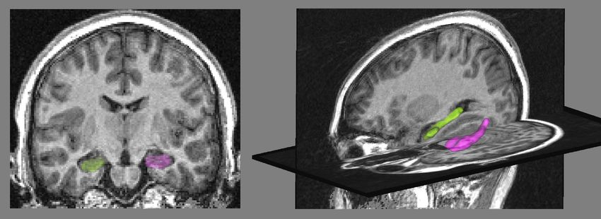
bioRxiv preprint first posted online Jul. 6, 2018; doi: http://dx.doi.org/10.1101/363861. The copyright holder for this preprint
 (which was not peer-reviewed) is the author/funder, who has granted bioRxiv a license to display the preprint in perpetuity.
                                It is made available under a CC-BY-ND 4.0 International license.

Cury et al.                                                                     Statistical shape analysis for large datasets

  A common approach in shape analysis is to analyse the deformations that map individuals to an atlas or
template, e.g. (1)(2)(3)(4)(5). The three main components of these approaches are the underlying defor-
mation model, the template estimation method and the statistical analysis itself. The Large Deformation
Diffeomorphic Metric Mapping (LDDMM) framework (6)(7)(8) provides a natural setting for quantifying
deformations between shapes or images. This framework provides diffeomorphic transformations which
preserve the topology and also provides a metric between shapes. The LDDMM framework is also a natu-
ral setting for estimating templates from a population of shapes, because such templates can be defined as
means in the induced shape space. Various methods have been proposed to estimate templates of a given
population using the LDDMM framework (4)(9)(10)(3). All methods are computationally expensive due
the complexity of the deformation model. This is a limitation for the study of large databases.
  In this paper, we present a fast approach for template-based statistical analysis of large datasets in the
LDDMM setting, and apply it to a population of 1000 hippocampal shapes. The template estimation is
based on diffeomorphic centroid approaches, which were introduced at the Geometric Science of Informa-
tion conference GSI13 (11, 12). The main idea of these methods is to iteratively update a centroid shape by
successive matchings to the different subjects. This procedure involves a limited number of matchings and
thus quickly provides a template estimation of the population. We previously showed that these centroids
can be used to initialize a variational template estimation procedure (12), and that even if the ordering of
the subject along itarations does affect the final result, all centres are very similar. Here, we propose to
use these centroid estimations directly for template-based statistical shape analysis. The analysis is done
on the tangent space to the template shape, either directly through Kernel Principal Component Analysis
(Kernel PCA (13)) or to approximate distances between subjects. We perform a thorough evaluation of
the approach using three datasets: one synthetic dataset and two real datasets composed of 50 and 1000
subjects respectively. In particular, we study extensively the impact of different centroids on statistical
analysis, and compare the results to those obtained using a standard variational template method. We will
also use the large database to predict, using the shape parameters extracted from a centroid estimation
of the population, some anatomical variations of the hippocampus in the normal population, called In-
complete Hippocampal Inversions and present in 17% of the normal population (14). IHI are also present
in temporal lobe epilepsy with a frequency around 50% (15), and is also involved in major depression
disorders (16).
  The paper is organized as follows. We first present in section 2 the mathematical frameworks of diffeo-
morphisms and currents, on which the approach is based, and then introduce the diffeomorphic centroid
methods in section 3. Section 4 presents the statistical analysis. The experimental evaluation of the method
is then presented in Section 5.

2 MATHEMATICAL FRAMEWORKS
Our approach is based on two mathematical frameworks which we will recall in this section. The Large
Deformation Diffeomorphic Metric Mapping framework is used to generate optimal matchings and quan-
tify differences between shapes. Shapes themselves are modelled using the framework of currents which
does not assume point-to-point correspondences and allows performing linear operations on shapes.
2.1 LDDMM framework
  Here we very briefly recall the main properties of the LDDMM setting. See (6, 7, 8) for more details.
The Large Deformation Diffeomorphic Metric Mapping framework allows analysing shape variability of
a population using diffeomorphic transformations of the ambient 3D space. It also provides a shape space
representation which means that shapes of the population are seen as points in an infinite dimensional
smooth manifold, providing a continuum between shapes.
  In the LDDMM framework, deformation maps ϕ : R3 → R3 are generated by integration of time-
dependent vector fields v(x, .), with x ∈ R3 and t ∈ [0, 1]. If v(x, t) is regular enough, i.e. if we consider
the vector fields (v(·, t))t∈[0,1] in L2 ([0, 1], V ), where V is a Reproducing Kernel Hilbert Space (RKHS)
embedded in the space of C 1 vector fields vanishing at infinity, then the transport equation:
                                   dφv
                                     dt (x, t) = v(φv (x, t), t) ∀t ∈ [0, 1]                               (1)
                                    φv (x, 0) = x                 ∀x ∈ R3

Preprint                                                                                                                            2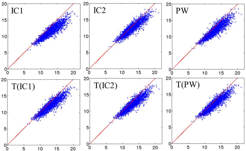
bioRxiv preprint first posted online Jul. 6, 2018; doi: http://dx.doi.org/10.1101/363861. The copyright holder for this preprint
  (which was not peer-reviewed) is the author/funder, who has granted bioRxiv a license to display the preprint in perpetuity.
                                 It is made available under a CC-BY-ND 4.0 International license.

Cury et al.                                                                     Statistical shape analysis for large datasets

has a unique solution, and one sets ϕv = φv (·, 1) the diffeomorphism induced by v(x, ·). The induced
set of diffeomorphisms AV is a subgroup of the group of C 1 diffeomorphisms. The regularity of velocity
fields is controlled by:
                                            Z 1
                                    E(v) :=      kv(·, t)k2V dt.                                    (2)
                                                                  0

 The subgroup of diffeomorphisms AV is equipped with a right-invariant metric defined by the rules:
∀ϕ, ψ ∈ AV ,
                       D(ϕ, ψ) = D(id, ψ ◦ ϕ−1 )

                                      R1                                                        (3)
                       D(id, ϕ) = inf{ 0 kv(·, t)kV dt, ϕ = φv (·, 1)}

i.e. the infimum is taken over all v ∈ L2 ([0, 1], V ) such that ϕv = ϕ. D(ϕ, ψ) represents the shortest
length of paths connecting ϕ to ψ in the diffeomorphisms group.
2.2 Momentum vectors
  In a discrete setting, when the matching criterion depends only on ϕv via the images ϕv (xp ) of a finite
number of points xp (such as the vertices of a mesh) one can show that the vector fields v(x, t) which
induce the optimal deformation map can be written via a convolution formula over the surface involving
the reproducing kernel KV of the RKHS V :
                                                            n
                                                            X
                                              v(x, t) =           KV (x, xp (t))αp (t),                                              (4)
                                                            p=1

where xp (t) = φv (xp , t) are the trajectories of points xp , and αp (t) ∈ R3 are time-dependent vectors
called momentum vectors, which completely parametrize the deformation. Trajectories xp (t) depend only
on these vectors as solutions of the following system of ordinary differential equations:
                                                           n
                                           dxq (t) X
                                                  =  KV (xq (t), xp (t))αp (t),                                                      (5)
                                             dt
                                                         p=1

for 1 ≤ q ≤ n. This is obtained by plugging formula 4 for the optimal velocity fields into the flow equation
1 taken at x = xq . Moreover, the norm of v(·, t) also takes an explicit form:
                                                    n X
                                                      n
                                 kv(·, t)k2V =
                                                    X
                                                               αp (t)T KV (xp (t), xq (t))αq (t).                                    (6)
                                                    p=1 q=1

Note that since V is a space of vector fields, its kernel KV (x, y) is in fact a 3×3 matrix for every x, y ∈ R3 .
However we will only consider scalar invariant kernels of the form KV (x, y) = h(kx − yk2 /σV2 )I3 , where
h is a real function (in our case we use the Cauchy kernel h(r) = 1/(1 + r)), and σV a scale factor. In
the following we will use a compact representation for kernels and vectors. For example equation 6 can
be written:
                                             kv(·, t)k2V = α(t)T KV (x(t))α(t),                                                      (7)

where α(t) = (αp (t))p=1...n , ∈ R3×n , x(t) = (xp (t))p=1...n , ∈ R3×n and KV (x(t)) the matrix of
KV (xp (t), xq (t)).
Geodesic shooting
  The minimization of the energy E(v) in matching problems can be interpreted as the estimation of a
length-minimizing path in the group of diffeomorphisms AV , and also additionally as a length-minimizing

Pre-print                                                                                                                             3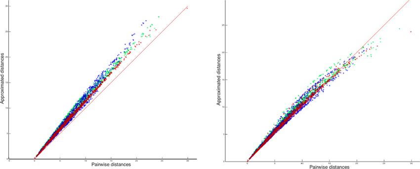
bioRxiv preprint first posted online Jul. 6, 2018; doi: http://dx.doi.org/10.1101/363861. The copyright holder for this preprint
 (which was not peer-reviewed) is the author/funder, who has granted bioRxiv a license to display the preprint in perpetuity.
                                It is made available under a CC-BY-ND 4.0 International license.

Cury et al.                                                                     Statistical shape analysis for large datasets

path in the space of point sets when considering discrete problems. Such length-minimizing paths obey
geodesic equations (see (3)) which write as follows:
                           (
                             dx(t)
                               dt = KV (x(t))α(t)                                                  (8)
                             dα(t)     1
                                                    T

                               dt = − 2 ∇x(t) α(t) KV (x(t))α(t) ,

Note that the first equation is nothing more than equation 5 which allows to compute trajectories xp (t)
from any time-dependent momentum vectors αp (t), while the second equation gives the evolution of
the momentum vectors themselves. This new set of ODEs can be solved from any initial conditions
(xp (0), αp (0)), which means that the initial momentum vectors αp (0) fully determine the subsequent
time evolution of the system (since the xp (0) are fixed points). As a consequence, these initial momentum
vectors encode all information of the optimal diffeomorphism. For example, the distance D(id, ϕ) satisfies

                            D(id, ϕ)2 = E(v) = kv(·, 0)k2V = α(0)T KV (x(0))α(0),                                                    (9)

We can also use geodesic shooting from initial conditions (xp (0), αp (0)) in order to generate any arbitrary
deformation of a shape in the shape space.
2.3 Shape representation: Currents
  The use of currents ((17, 18)) in computational anatomy was introduced by J. Glaunès and M. Vaillant
in 2005 (19)(20) and subsequently developed by Durrleman ((21)). The basic idea is to represent surfaces
as currents, i.e. linear functionals on the space of differential forms and to use kernel norms on the dual
space to express dissimilarities between shapes. Using currents to represent surfaces has some benefits.
First it avoids the point correspondence issue: one does not need to define pairs of corresponding points
between two surfaces to evaluate their spatial proximity. Moreover, metrics on currents are robust to dif-
ferent samplings and topological artefacts and take into account local orientations of the shapes. Another
important benefit is that this model embeds shapes into a linear space (the space of all currents), which
allows considering linear combinations such as means of shapes in the space of currents.
  Let us briefly recall this setting. For sake of simplicity we present currents as linear forms acting on
vector fields rather than differential forms which are an equivalent formulation in our case. Let S be an
oriented compact surface, possibly with boundary. Any smooth vector field w of R3 can be integrated over
S via the rule:
                                            Z
                                  [S](w) =     h w(x) , n(x) i dσS (x),                               (10)
                                                            S

with n(x) the unit normal vector to the surface, dσS the Lebesgue measure on the surface S, and [S] is
called a 2-current associated to S.
  Given an appropriate Hilbert space (W ,h · , · iW ) of vector fields, continuously embedded in C01 (R3 , R3 ),
the space of currents we consider is the space of continuous linear forms on W , i.e. the dual space W ∗ .
For any point x ∈ R3 and vector α ∈ R3 one can consider the Dirac functional δxα : w 7→ h w(x) , α i
which belongs to W ∗ . The Riesz representation theorem states that there exists a unique u ∈ W such
that for all w ∈ W , h u , w iW = δxα (w) = h w(x) , α i. u is thus a vector field which depends on x and
linearly on α, and we write it u = KW (·, x)α. KW (x, y) is a 3 × 3 matrix, and KW : R3 × R3 → R3×3
the mapping called the reproducing kernel of the space W . Thus we have the rule
                                                 hKW (·, x)α, wiW = h w(x) , α i .

Moreover, applying this formula to w = KW (·, y)β for any other point y ∈ R3 and vector β ∈ R3 , we get

                           hKW (·, x)α, KW (·, y)βiW               = h KW (x, y)β , α i                                             (11)
                                                                                                   D               E
                                                                   = αT KW (x, y)β =                   δxα , δyβ
                                                                                                                       W∗

Preprint                                                                                                                              4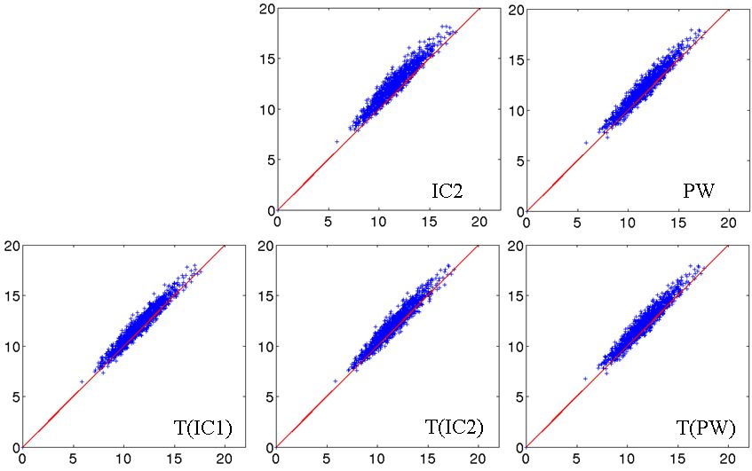
bioRxiv preprint first posted online Jul. 6, 2018; doi: http://dx.doi.org/10.1101/363861. The copyright holder for this preprint
  (which was not peer-reviewed) is the author/funder, who has granted bioRxiv a license to display the preprint in perpetuity.
                                 It is made available under a CC-BY-ND 4.0 International license.

Cury et al.                                                                     Statistical shape analysis for large datasets

Using equation 11, one can prove that for two surfaces S and T ,
                                                       Z Z
  h [S] , [T ] iW ∗                  =                           h nS (x) , KW (x, y)nT (y) i                        dσS (x)dσT (y) (12)
                                                         S   T

This formula defines the metric we use as data attachment term for comparing surfaces. More precisely,
the difference between two surfaces is evaluated via the formula:

                     k[S] − [T ]k2W ∗ = h [S] , [S] iW ∗ + h [T ] , [T ] iW ∗ − 2 h [S] , [T ] iW ∗                                  (13)

The type of kernel fully determines the metric and therefore will have a direct impact on the behaviour of
the algorithms. We use scalar invariant kernels of the form KW (x, y) = h(kx − yk2 /σW  2 )I , where h is a
                                                                                            3
real function (in our case we use the Cauchy kernel h(r) = 1/(1 + r)), and σW a scale factor.
 Note that the varifold (22) can be also use for shape representation without impacting the methodology.
The shapes we used for this study are well represented by currents.
2.4 Surface matchings

 We can now define the optimal match between two currents [S] and [T ], which is the diffeomorphism
minimizing the functional

                                         JS,T (v) = γE(v) + k[ϕv (S)] − [T ]k2W ∗                                                    (14)

This functional is non convex and in practice we use a gradient descent algorithm to perform the opti-
mization, which cannot guarantee to reach a global minimum. We observed empirically that local minima
can be avoided by using a multi-scale approach in which several optimization steps are performed with
decreasing values of the width σW of the kernel KW (each step provides an initial guess for the next one).
Evaluations of the functional and its gradient require numerical integrations of high-dimensional ordinary
differential equations (see equation 5), which is done using Euler trapezoidal rule. Note that three impor-
tant parameters control the matching process: γ controls the regularity of the map, σV controls the scale
in the space of deformations and σW controls the scale in the space of currents.
2.5 GPU implementation

  To speed up the matchings computation of all methodes used in this study (the variational template
and the different centroid estimation algorithms), we use a GPU implementation for the computation of
kernel convolutions. This computation constitutes the most time-consuming part of LDDMM methods.
Computations were performed on a Nvidia Tesla C1060 card. The GPU implementation can be found here:
http://www.mi.parisdescartes.fr/~glaunes/measmatch/measmatch040816.zip

3 DIFFEOMORPHIC CENTROIDS
Computing a template in the LDDMM framework can be highly time consuming, taking a few days or
some weeks for large real-world databases. Here we propose a fast approach which provides a centroid
correctly centred among the population.
3.1 General idea

 The LDDMM framework, in an ideal setting (exact matching between shapes), sets the template esti-
mation problem as a centroid computation on a Riemannian manifold. The Fréchet mean is the standard
way for defining such a centroid and provides the basic inspiration of all LDDMM template estimation
methods.

Pre-print                                                                                                                              5
bioRxiv preprint first posted online Jul. 6, 2018; doi: http://dx.doi.org/10.1101/363861. The copyright holder for this preprint
(which was not peer-reviewed) is the author/funder, who has granted bioRxiv a license to display the preprint in perpetuity.
It is made available under a CC-BY-ND 4.0 International license.
Cury et al. Statistical shape analysis for large datasets
If xi , 1 ≤ i ≤ N are points in Rd , then their centroid is defined as
N
N 1 X i
b = x. (15)
N
i=1
It also satisfies the following two alternative characterizations:
X
bN = arg min ky − xi k2 . (16)
y∈Rd 1≤i≤N
and
1
b = x1
(17)
bk+1 = k+1
k
bk + 1
k+1 x
k+1 , 1 ≤ k ≤ N − 1.
Now, when considering points xi living on a Riemannian manifold M (we assume M is path-connected
and geodesically complete), the definition of bN cannot be used because M is not a vector space. However
the variational characterization of bN as well as the iterative characterization, both have analogues in the
Riemannian case. The Fréchet mean is defined under some hypotheses (see (23)) on the relative locations
of points xi in the manifold:
X
bN = arg min dM (y, xi )2 . (18)
y∈M 1≤i≤N
Many mathematical studies (as for example Kendall (24), Karcher (25) Le (26), Afsari (27, 28), Ar-
naudon (23)), have focused on proving the existence and uniqueness of the mean, as well as proposing
algorithms to compute it. However, these approaches are computationally expensive, in particular in high
dimension and when considering non trivial metrics. An alternative idea consists in using the Riemannian
analogue of the second characterization:
( 1
b̃ = x1
k+1 k 1
(19)
b̃ = geod(b̃ , xk+1 , k+1 ), 1 ≤ k ≤ N − 1,
where geod(y, x, t) is the point located along the geodesic from y to x, at a distance from y equal to t
times the length of the geodesic. This does not define the same point as the Fréchet mean, and moreover
the result depends on the ordering of the points. In fact, all procedures that are based on decomposing
the Euclidean equality bN = N1 N i
P
i=1 x as a sequence of pairwise convex combinations lead to possible
alternative definitions of centroid in a Riemannian setting. However, this should lead to a fast estimation.
We hypothesize that, in the case of shape analysis, it could be sufficient for subsequent template based
statistical analysis. Moreover, this procedure has the side benefit that at each step bk is the centroid of the
xi , 1 ≤ i ≤ k.
In the following, we present three algorithms that build on this idea. The two first methods are iterative,
and the third one is recursive, but also based on pairwise matchings of shapes.
3.2 Direct Iterative Centroid (IC1)
The first algorithm roughly consists in applying the following procedure: given a collection of N shapes
Si , we successively update the centroid by matching it to the next shape and moving along the geodesic
flow. More precisely, we start from the first surface S1 , match it to S2 and set B2 = φv1 (S1 , 1/2). B2
represents the centroid of the first two shapes, then we match B2 to S3 , and set as B3 = φv2 (B2 , 1/3).
Then we iterate this process (see Algorithm 1).
Preprint 6bioRxiv preprint first posted online Jul. 6, 2018; doi: http://dx.doi.org/10.1101/363861. The copyright holder for this preprint
(which was not peer-reviewed) is the author/funder, who has granted bioRxiv a license to display the preprint in perpetuity.
It is made available under a CC-BY-ND 4.0 International license.
Cury et al. Statistical shape analysis for large datasets
Data: N surfaces Si
Result: 1 surface BN representing the centroid of the population
B1 = S1 ;
for i from 1 to N − 1 do
Bi is matched to Si+1 which results in a deformation map φvi (x, t);
1
Set Bi+1 = φvi (Bi , i+1 ) which means that we transport Bi along the geodesic and stop at time
1
t = i+1 ;
end
Algorithm 1: Iterative Centroid 1 (IC1)
Figure 1. Diagrams of the iterative processes which lead to the centroids computations. The tops of
the diagrams represent the final centroid. The diagram on the left corresponds to the Iterative Centroid
algorithms (IC1 and IC2). The diagram on the right corresponds to the pairwise algorithm (PW).
3.3 Centroid with averaging in the space of currents (IC2)
Because matchings are not exact, the centroid computed with the IC1 method accumulates small errors
which can have an impact on the final centroid. Furthermore, the final centroid is in fact a deformation
of the first shape S1 , which makes the procedure even more dependent on the ordering of subjects than
it would be in an ideal exact matching setting. In this second algorithm, we modify the updating step
by computing a mean in the space of currents between the deformation of the current centroid and the
backward flow of the current shape being matched. Hence the computed centroid is not a surface but a
combination of surfaces, as in the template estimation method. The algorithm proceeds as presented in
Algorithm 2.
Data: N surfaces Si
Result: 1 current BN representing the centroid of the population
B1 = [S1 ];
for i from 1 to N − 1 do
Bi is matched to [Si+1 ] which results in a deformation map φvi (x, t);
i 1 1 i
Set Bi+1 = i+1 φvi (Bi , i+1 ) + i+1 [φui (Si+1 , i+1 )] which means that we transport Bi along the
1
geodesic and stop at time t = i+1 ;
where ui (x, t) = −v i (x, 1 − t), i.e. φui is the reverse flow map.
end
Algorithm 2: Iterative Centroid 2 (IC2)
The weights in the averaging reflect the relative importance of the new shape, so that at the end of the
procedure, all shapes forming the centroid have equal weight N1 .
1
Note that we have used the notation φvi (Bi , i+1 ) to denote the transport (push-forward) of the current
Bi by the diffeomorphism. Here Bi is a linear combination of currents associated to surfaces, and the
Pre-print 7bioRxiv preprint first posted online Jul. 6, 2018; doi: http://dx.doi.org/10.1101/363861. The copyright holder for this preprint
(which was not peer-reviewed) is the author/funder, who has granted bioRxiv a license to display the preprint in perpetuity.
It is made available under a CC-BY-ND 4.0 International license.
Cury et al. Statistical shape analysis for large datasets
transported current is the linear combination (keeping the weights unchanged) of the currents associated
to the transported surfaces.
3.4 Alternative method : Pairwise Centroid (PW)
Another possibility is to recursively split the population in two parts until having only one surface in
each group (see Fig. 1), and then going back up along the dyadic tree by computing pairwise centroids
between groups, with appropriate weight for each centroid (Algorithm 3).
Data: N surfaces Si
Result: 1 surface B representing the centroid of the population
if N ≥ 2 then
Blef t = Pairwise Centroid (S1 , ..., S[N/2] );
Bright = Pairwise Centroid (S[N/2]+1 , ..., SN );
Blef t is matched to Bright which results in a deformation map φv (x, t);
Set B = φv (Blef t , [N/2]+1
N ) which means we transport Blef t along the geodesic and stop at time
[N/2]+1
t= N ;
end
else
B = S1
end
Algorithm 3: Pairwise Centroid (PW)
These three methods depend on the ordering of subjects. In a previous work (12), we showed empirically
that different orderings result in very similar final centroids. Here we focus on the use of such centroid for
statistical shape analysis.
3.5 Comparison with a variational template estimation method
In this study, we will compare our centroid approaches to a variational template estimation method
proposed by Glaunès et al (10). This variational method estimates a template given a collection of surfaces
using the framework of currents. It is posed as a minimum mean squared error estimation problem. Let Si
be N surfaces in R3 (i.e. the whole surface population). Let [Si ] be the corresponding current of Si , or its
approximation by a finite sum of vectorial Diracs. The problem is formulated as follows:
n o N
X
kT − [ϕvi (Si )] k2W ∗ + γE(vi ) ,
vˆi , T̂ = arg min (20)
vi ,T i=1
The method uses an alternated optimization i.e. surfaces are successively matched to the template, then
the template is updated and this sequence is iterated until convergence. One can observe that when ϕi
is fixed, the functional is minimized when T is the average of [ϕi (Si )]: T = N1 N
P
i=1 [ϕvi (Si )] , which
makes the optimization with respect to T straightforward. This optimal current is the union of all surfaces
ϕvi (Si ). However, all surfaces being co-registered, the ϕ̂vi (Si ) are close to each other, which makes
the optimal template T̂ close to being a true surface. Standard initialization consists in setting T =
1 PN
N i=1 [Si ], which means that the initial template is defined as the combination of all unregistered shapes
in the population. Alternatively, if one is given a good initial guess T , the convergence speed of the method
can be improved. In particular, the initialisation can be provided by iterative centroids; this is what we
will use in the experimental section.
Regarding the computational complexity, the different centroid approaches perform N − 1 matchings
while the variational template estimation requires N × iter matchings, where iter is the number of iter-
ations. Moreover the time for a given matching depends quadratically on the number of vertices of the
surfaces being matched. It is thus more expensive when the template is a collection of surfaces as in IC2
and in the variational template estimation.
Preprint 8bioRxiv preprint first posted online Jul. 6, 2018; doi: http://dx.doi.org/10.1101/363861. The copyright holder for this preprint
(which was not peer-reviewed) is the author/funder, who has granted bioRxiv a license to display the preprint in perpetuity.
It is made available under a CC-BY-ND 4.0 International license.
Cury et al. Statistical shape analysis for large datasets
4 STATISTICAL ANALYSIS
The proposed iterative centroid approaches can be used for subsequent statistical shape analysis of
the population, using various strategies. A first strategy consists in analysing the deformations be-
tween the centroid and the individual subjects. This is done by analysing the initial momentum vectors
αi (0) = (αpi (0))p=1...n ∈ R3×n which encode the optimal diffeomorphisms computed from the matching
between a centroid and the subjects Si . Initial momentum vectors all belong to the same vector space and
are located on the vertices of the centroid. Different approaches can be used to analyse these momentum
vectors, including Principal Component Analysis for the description of populations, Support Vector Ma-
chines or Linear Discriminant Analysis for automatic classification of subjects. A second strategy consists
in analysing the set of pairwise distances between subjects. Then, the distance matrix can be entered into
analysis methods such as Isomap (29), Locally Linear Embedding (30), (31) or spectral clustering algo-
rithms (32). Here, we tested two approaches: i) the analysis of initial momentum vectors using a Kernel
Principal Component Analysis for the first strategy; ii) the approximation of pairwise distance matrices
for the second strategy. These tests allow us both to validate the different iterative centroid methods and
to show the feasibility of such analysis on large databases.
4.1 Principal Component Analysis on initial momentum vectors
The Principal Component Analysis (PCA) on initial momentum vectors from the template to the subjects
of the population is an adaptation of PCA in which Euclidean scalar products between observations are
replaced by scalar products using a kernel. Here the kernel is KV the kernel of the R.K.H.S V . This
adaptation can be seen as a Kernel PCA (13). PCA on initial momentum vectors has previously been used
in morphometric studies in the LDDMM setting (3, 33) and it is sometimes referred to tangent PCA.
We briefly recall that, in standard PCA, the principal components of a dataset of N observations ai ∈ RP
with i ∈ {1, . . . , N } are defined by the eigenvectors of the covariance matrix C with entries:
1
C(i, j) = (ai − ā)t (aj − ā) (21)
N −1
1 PN i
with ai given as a column vector, ā = N
t
i=1 a , and x denotes the transposition of a vector x.
In our case, our observations are initial momentum vectors αi ∈ R3×n and instead of computing the
Euclidean scalar product in R3×n , we compute the scalar product with matrix KV , which is a natural
choice since it corresponds to the inner product of the corresponding initial vector fields in the space V .
The covariance matrix then writes:
1
CV (i, j) = (αi − ᾱ)t KV (x)(αj − ᾱ) (22)
N −1
with ᾱ the vector of the mean of momentum vectors, and x the vector of vertices of the template surface.
We denote λ1 , λ2 , . . . , λN the eigenvalues of C in decreasing order, and ν 1 , ν 2 , . . . , ν N the corresponding
eigenvectors. The k-th principal mode is computed from the k-th eigenvector ν k of CV , as follows:
N
X
mk = ᾱ + νjk (αj − ᾱ). (23)
j=1
The cumulative explained variance CEVk for the k first principal modes is given by the equation:
Pk
h=1 λh
CEVk = PN (24)
h=1 λh
We can use geodesic shooting along any principal mode mk to visualise the corresponding deformations.
Pre-print 9bioRxiv preprint first posted online Jul. 6, 2018; doi: http://dx.doi.org/10.1101/363861. The copyright holder for this preprint
(which was not peer-reviewed) is the author/funder, who has granted bioRxiv a license to display the preprint in perpetuity.
It is made available under a CC-BY-ND 4.0 International license.
Cury et al. Statistical shape analysis for large datasets
Remark
To analyse the population, we need to know the initial momentum vectors αi which correspond to
the matchings from the centroid to the subjects. For the IC1 and PW centroids, these initial momentum
vectors were obtained by matching the centroid to each subject. For the IC2 centroid, since the mesh
structure is composed of all vertices of the population, it is too computationally expensive to match the
centroid toward each subject. Instead, from the deformation of each subject toward the centroid, we used
the opposite vector of final momentum vectors for the analysis. Indeed, if we have two surfaces S and T
and need to compute the initial momentum vectors from T to S, we can estimate the initial momentum
vectors αT S (0) from T to S by computing the deformation from S to T and using the initial momentum
vectors α̃T S (0) = −αST (1), which are located at vertices φST (xS ).
4.2 Distance matrix approximation
Various methods such as Isomap (29) or Locally Linear Embedding (30) (31) use as input a matrix of
pairwise distances between subjects. In the LDDMM setting, it can be computed using diffeomorphic dis-
tances: ρ(Si , Sj ) = D(id, ϕij ). However, for large datasets, computing all pairwise deformation distance
is computationally very expensive, as it involves O(N 2 ) matchings. An alternative is to approximate the
pairwise distance between two subjects through their matching from the centroid or template. This ap-
proach has been introduced in Yang et al (34). Here we use a first order approximation to estimate the
diffeomorphic distance between two subjects:
q
ρ̃(Si , Sj ) = h αj (0) − αi (0) , KV (x(0))(αj (0) − αi (0) i, (25)
with x(0) the vertices of the estimated centroid or template and αi (0) is the vector of initial momentum
vectors computed by matching the template to Si . Using such approximation allows to compute only N
matchings instead of N (N − 1).
Note that ρ(Si , Sj ) is in fact the distance between Si and ϕij (Si ), and not between Si and Sj due to
the not exactitude of matchings. However we will refer to it as a distance in the following to denote the
dissimilarity between Si and Sj .
5 EXPERIMENTS AND RESULTS
In this section, we evaluate the use of iterative centroids for statistical shape analysis. Specifically, we
investigate the centring of the centroids within the population, their impact on population analysis based
on Kernel PCA and on the computation of distance matrices. For our experiments, we used three different
datasets: two real datasets and a synthetic one. In all datasets shapes are hippocampi. The hippocampus
is an anatomical structure of the temporal lobe of the brain, involved in different memory processes.
5.1 Data
The two real datasets are from the Euro-
pean database IMAGEN (36) 1 composed of
young healthy subjects. We segmented the hip-
pocampi from T1-weighted Magnetic Resonance
Images (MRI) of subjects using the SACHA soft-
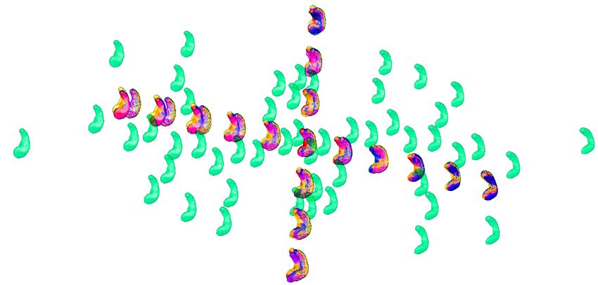
ware (35) (see Fig. 2). The synthetic dataset was
built using deformations of a single hippocampal
shape of the IMAGEN database. Figure 2. Left panel: coronal view of the MRI with
the binary masks of hippocampi segmented by the
The synthetic dataset SD SACHA software (35), the right hippocampus is in
is composed of synthetic deformations of a green and the left one in pink. Right panel: 3D view
single shape S0 , designed such that this single of the hippocampus meshes.
1 http://www.imagen-europe.com/
Preprint 10bioRxiv preprint first posted online Jul. 6, 2018; doi: http://dx.doi.org/10.1101/363861. The copyright holder for this preprint
(which was not peer-reviewed) is the author/funder, who has granted bioRxiv a license to display the preprint in perpetuity.
It is made available under a CC-BY-ND 4.0 International license.
Cury et al. Statistical shape analysis for large datasets
shape becomes the exact center of the population.
We will thus be able to compare the computed
centroids to this exact center. We generated 50
subjects for this synthetic dataset from S0 , along
geodesics in different directions. We randomly chose two orthogonal momentum vectors β 1 and β 2 in
R3×n . We then computed momentum vectors αi , i ∈ {1, . . . , 25} of the form k1i β 1 + k2i β 2 + k3i β 3 with
(k1i , k2i , k3i ) ∈ R3 , ∀i ∈ {1, . . . , 25}, kji ∼ N (0, σj ) with σ1 > σ2
σ3 and β 3 a randomly selected
momentum vector, adding some noise to the generated 2D space. We computed momentum vectors αj ,
j ∈ {26, . . . , 50} such as αj = −αj−25 . We generated the 50 subjects of the population by computing
geodesic shootings of S0 using the initial momentum vectors αi , i ∈ {1, . . . , 50}. The population is sym-
metrical since 50 i
P
i α = 0. It should be noted that all shapes of the dataset have the same mesh structure
composed of n = 549 vertices.
The real dataset RD50
is composed of 50 left hippocampi from the IMAGEN database. We applied the following preprocessing
steps to each individual MRI. First, the MRI was linearly registered toward the MNI152 atlas, using the
FLIRT procedure (37) of the FSL software 2 . The computed linear transformation was then applied to the
binary mask of the hippocampal segmentation. A mesh of this segmentation was then computed from the
binary mask using the BrainVISA software 3 . All meshes were then aligned using rigid transformations
to one subject of the population. For this rigid registration, we used a similarity term based on measures
(as in (38)). All meshes were decimated in order to keep a reasonable number of vertices: meshes have on
average 500 vertices.
The real database RD1000
is composed of 1000 left hippocampi from the IMAGEN database. We applied the same preprocessing
steps to the MRI data as for the dataset RD50. This dataset has also a score of Incomplete Hippocampal
Inversion (IHI) (14), which is an anatomical variant of the hippocampus, present in 17% of the normal
population.
5.2 Experiments
For the datasets SD and RD50 (which both contain 50 subjects), we compared the results of the three
different iterative centroid algorithms (IC1, IC2 and PW). We also investigated the possibility of comput-
ing variational templates, initialized by the centroids, based on the approach presented in section 3.5. We
could thus compare the results obtained when using the centroid directly to those obtained when using
the most expensive (in term of computation time) template estimation. We thus computed 6 different cen-
tres: IC1, IC2, PW and the corresponding variational templates T(IC1), T(IC2), T(PW). For the synthetic
dataset SD, we could also compare those 6 estimated centres to the exact centre of the population. For the
real dataset RD1000 (with 1000 subjects), we only computed the iterative centroid IC1.
For all computed centres and all datasets, we investigated: 1) the computation time; 2) whether the
centres are close to a critical point of the Fréchet functional of the manifold discretised by the population;
3) the impact of the estimated centres on the results of Kernel PCA; 4) their impacts on approximated
distance matrices.
To assess the "centring" (i.e. how close an estimated centre is to a critical point of the Fréchet functional)
of the different centroids and variational templates, we computed a ratio using the momentum vectors from
centres to subjects. The ratio R takes values between 0 and 1:
k N1 N v i (·, 0)kV
P
R = 1 PNi=1 , (26)
kv i (·, 0)k
N i=1 V
2 http://fsl.fmrib.ox.ac.uk/fsl/fslwiki/FslOverview
3 http://www.brainvisa.info
Pre-print 11bioRxiv preprint first posted online Jul. 6, 2018; doi: http://dx.doi.org/10.1101/363861. The copyright holder for this preprint
(which was not peer-reviewed) is the author/funder, who has granted bioRxiv a license to display the preprint in perpetuity.
It is made available under a CC-BY-ND 4.0 International license.
Cury et al. Statistical shape analysis for large datasets
with v i (·, 0) the vector field of the deformation from the estimated centre to the subject Si , corresponding
to the vector of initial momentum vectors αi (0).
We compared the results of Kernel PCA computed from these different centres by comparing the
principal modes and the cumulative explained variance for different number of dimensions.
Finally, we compared the approximated distance matrices to the direct distance matrix.
For the RD1000 dataset, we will try to predict an anatomical variant of the normal population, the
Incomplete Hippocampal Inversion (IHI), presents in only 17% of the population.
5.3 Synthetic dataset SD
5.3.1 Computation time
All the centroids and variational templates have been computed with σV = 15, which represents roughly
half of the shapes length. Computation times for IC1 took 31 minutes, 85 minutes for IC2, and 32 minutes
for PW. The corresponding variational template initialised by these estimated centroids took 81 minutes
(112 minutes in total), 87 minutes (172 minutes in total) and 81 minutes (113 minutes in total). As a
reference, we also computed a template with the standard initialisation whose computation took 194
minutes. Computing a centroid saved between 56% and 84% of computation time over the template with
standard initialization and between 50% and 72% over the template initialized by the centroid.
5.3.2 "Centring" of the estimated centres
Since in practice a computed centre is never at the exact centre, and its estimation may vary accordingly
to the discretisation of the underlying shape space, we decided to generate another 49 populations, so
we have 50 different discretisations of the shape space. For each of these populations, we computed
the 3 centroids and the 3 variational templates initialized with these centroids. We calculated the ratio
R described in the previous section for each estimated centre. Table 1 presents the mean and standard
deviation values of the ratio R for each centroid and template, computed over these 50 populations.
In a pure Riemannian setting (i.e. disregarding the fact
that matchings are not exact), a zero ratio would mean Table 1. Synthetic dataset SD. Ratio R
that we are at a critical point of the Fréchet functional, (equation 26) computed for the 3 centroids
and under some reasonable assumptions on the curvature C, and the 3 variational templates initialized
of the shape space in the neighbourhood of the dataset via these centroids (T (C)).
(which we cannot check however), it would mean that Ratio C T (C)
we are at the Fréchet mean. By construction, the ratio IC1 0.07 ± 0.03 0.05 ± 0.02
computed from the exact centre using the initial momen- IC2 0.07 ± 0.03 0.05 ± 0.02
tum vectors αi used for the construction of subjects Si PW 0.11 ± 0.05 0.07 ± 0.02
(as presented in section 5.1) is zero.
Ratios R are close to zero for all centroids and varia-
tional templates, indicating that they are close to the exact
centre. Furthermore, the value of R may be partly due to the non-exactitude of the matchings between
the estimated centres and the subjects. To become aware of this non-exactitude, we matched the exact
centre toward all subjects of the SD dataset. The resulting ratio is R = 0.05. This is of the same order of
magnitude as the ratios obtained in Table 1, indicating that the estimated centres are indeed very close to
the exact centre.
5.3.3 PCA on initial momentum vectors
We performed a PCA computed with the initial momentum vectors (see section 4 for details) from our
different estimated centres (3 centroids, 3 variational templates and the exact centre).
We computed the cumulative explained variance for different number of dimensions of the PCA. Results
are presented in Table 2. The cumulative explained variances are very similar for the different centres for
any number of dimensions.
Preprint 12bioRxiv preprint first posted online Jul. 6, 2018; doi: http://dx.doi.org/10.1101/363861. The copyright holder for this preprint
(which was not peer-reviewed) is the author/funder, who has granted bioRxiv a license to display the preprint in perpetuity.
It is made available under a CC-BY-ND 4.0 International license.
Cury et al. Statistical shape analysis for large datasets
Table 2. Synthetic dataset SD. Proportion of cumulative explained variance of kernel PCA computed
from different centres.
1st mode 2nd mode 3rd mode
Centre 0.829 0.989 0.994
IC1 0.829 0.990 0.995
IC2 0.833 0.994 0.996
PW 0.829 0.990 0.995
T(IC1) 0.829 0.995 0.999
T(IC2) 0.829 0.995 0.999
T(PW) 0.829 0.995 0.999
Figure 3. Synthetic dataset SD. Illustration of the two principal components of the 6 centres projected
into the 2D space of the SD dataset. Synthetic population in green, the real centre is in red in the middle.
The two axes are the two principal components projected into the 2D space of the population computed
from 7 different estimated centres (marked in orange for the exact centre, in blue for IC1, in yellow for
IC2 and in magenta for PW), they go from −2σ to +2σ of the variability of the corresponding axe. This
figure shows that the 6 different tangent spaces projected into the 2D space of shapes, are very similar,
even if the centres have different positions.
We wanted to take advantage of the construction of this synthethic dataset to answer the question:
Do the principal components explain the same deformations? The SD dataset allows to visualise the
principal component relatively to the real position of the generator vectors and the population itself. Such
visualisation is not possible for real dataset since shape spaces are not generated by only 2 vectors. For this
synthetic dataset, we can project principal components on the 2D space spanned by β1 and β2 as described
in the previous paragraph. This projection allows displaying in the same 2D space subjects in their native
space, and principal axes computed from the different Kernel PCAs. To visualize the first component
(respectively
√ the √ second one),√we shot from the associated centre in the direction k ∗ m1 (resp. m2 ) with
k ∈ [−2 λ1 ; +2 λ1 ] (resp. λ2 ). Results are presented in Figure 3. The deformations captured by the 2
principal axes are extremely similar for all centres. The principal axes for the 7 centres, have all the same
position within the 2D shape space. So for a similar amount of explained variance, the axes describe the
same deformation.
Overall, for this synthetic dataset, the 6 estimated centres give very similar PCA results.
5.3.4 Distance matrices
We then studied the impact of different centres on the approximated distance matrices. We computed the
seven approximated distance matrices corresponding to the seven centres, and the direct pairwise distance
Pre-print 13bioRxiv preprint first posted online Jul. 6, 2018; doi: http://dx.doi.org/10.1101/363861. The copyright holder for this preprint
(which was not peer-reviewed) is the author/funder, who has granted bioRxiv a license to display the preprint in perpetuity.
It is made available under a CC-BY-ND 4.0 International license.
Cury et al. Statistical shape analysis for large datasets
Table 3. Synthetic dataset SD. Mean ± standard deviation errors e (equation 27) between the six
different approximated distance matrices for each of the generated data sets.
e(aM (.), aM (.)) IC2 PW T(IC1) T(IC2) T(PW)
IC1 0.001 ± 0.001 0.002 ± 0.002 0.084 ± 0.02 0.084 ± 0.02 0.084 ± 0.02
IC2 0 0.003 ± 0.002 0.084 ± 0.02 0.084 ± 0.02 0.084 ± 0.02
PW 0 0.084 ± 0.02 0.084 ± 0.02 0.084 ± 0.02
T(IC1) 0 0.001 ± 0.001 0.002 ± 0.001
T(IC2) 0 0.002 ± 0.001
Figure 4. Synthetic datasets generated from SD50. Left: scatter plot between the approximated dis-
tance matrices aM (T (IC1)) of 3 different populations, and the pairwise distances matrices of the
corresponding population. Right: scatter plot between the approximated distance matrices aM (IC1) of 3
different populations, and the pairwise distances matrices of the corresponding population. The red line
corresponds to the identity.
matrix computed by matching all subjects to each other. Computation of the direct distance matrix took
1000 minutes (17 hours) for this synthetic dataset of 50 subjects. In the following, we denote as aM (C)
the approximated distance matrix computed from the centre C.
To quantify the difference between these matrices, we used the following error e:
N
1 X |M1 (i, j) − M2 (i, j)|
e(M1 , M2 ) = 2 (27)
N max(M1 (i, j), M2 (i, j))
i,j=1
with M1 and M2 two distance matrices. Results are reported in Table 3. For visualisation of the errors
against the pairwise computed distance matrices, we also computed the error between the direct distance
matrix, by computing pairwise deformations (23h hours of computation per population), for 3 popula-
tions randomly selected. Figure 4 shows scattered plots between the pairwise distances matrices and the
approximated distances matrices of IC1 and T(IC1) for the 3 randomly selected populations. The errors
between the aM (IC1) and the pairwise distance matrices of each of the populations are 0.17 0.16 and
0.14, respectively 0.11 0.08 and 0.07 for the errors with the corresponding aM (T (IC1)). We can ob-
serve a subtle curvature of the scatter-plot, which is due to the curvature of the shape space. This figure
illustrates the good approximation of the distances matrices, regarding to the pairwise estimation distance
matrix. The variational templates are getting slightly closer to the identity line, which is expected (as for
the better ratio values) since they have extra iterations to converge to a centre of the population, however
the estimated centroids from the different algorithms, still provide a good approximation of the pairwise
distances of the population. In conclusion for this set of synthetic population, the different estimated
centres have also a little impact on the approximation of the distance matrices.
Preprint 14bioRxiv preprint first posted online Jul. 6, 2018; doi: http://dx.doi.org/10.1101/363861. The copyright holder for this preprint
(which was not peer-reviewed) is the author/funder, who has granted bioRxiv a license to display the preprint in perpetuity.
It is made available under a CC-BY-ND 4.0 International license.
Cury et al. Statistical shape analysis for large datasets
Table 4. Real dataset RD50. Proportion of cumulative explained variance for kernel PCAs computed
from the 6 different centres, for different number of dimensions
1st mode 2nd mode 15th mode 20th mode
IC1 0.118 0.214 0.793 0.879
IC2 0.121 0.209 0.780 0.865
PW 0.117 0.209 0.788 0.875
T(IC1) 0.117 0.222 0.815 0.899
T(IC2) 0.115 0.220 0.814 0.898
T(PW) 0.116 0.221 0.814 0.898
5.4 The real dataset RD50
We now present experiments on the real dataset RD50. For this dataset, the exact center of the population
is not known, neither is the distribution of the population and meshes have different numbers of vertices
and different connectivity structures.
5.4.1 Computation time
We estimated our 3 centroids IC1 (75 minutes) IC2 (174 minutes) and PW (88 minutes), and the corre-
sponding variational templates, which took respectively 188 minutes, 252 minutes and 183 minutes. The
total computation time for T (IC1) is 263 minutes, 426 minutes for T (IC2) and 271 minutes for T (P W ).
For comparison of computation time, we also computed a template using the standard initialization (the
whole population as initialisation) which took 1220 minutes (20.3 hours). Computing a centroid saved
between 85% and 93% of computation time over the template with standard initialization and between
59% and 71% over the template initialized by the centroid.
5.4.2 Centring of the centres
As for the synthetic dataset, we assessed the centring of these six different centres. To that purpose,
we first computed the ratio R of equation (26), for the centres estimated via the centroids methods, IC1
has a R = 0.25, for IC2 the ratio is R = 0.33 and for PW it is R = 0.32. For centres estimated via
the variational templates initialised by those centroids, the ratio for T(IC1) is R = 0.21, for T(IC2) is
R = 0.31 and for T(PW) is R = 0.26.
The ratios are higher than for the synthetic dataset indicating that centres are less centred. This was
predictable since the population is not built from one surface via geodesic shootings as the synthetic
dataset. In order to better understand these values, we computed the ratio for each subject of the population
(after matching each subject toward the population), as if each subject was considered as a potential centre.
For the whole population, the average ratio was 0.6745, with a minimum of 0.5543, and a maximum of
0.7626. These ratios are larger than the one computed for the estimated centres and thus the 6 estimated
centres are closer to a critical point of the Frechet functional than any subject of the population.
5.4.3 PCA on initial momentum vectors
As for the synthetic dataset, we performed six PCAs from the estimated centres.
Figure 5 and Table 4 show the proportion of cumulative explained variance for different number of
modes. We can note that for any given number of modes, all PCAs result in the same proportion of
explained variance.
5.4.4 Distance matrices
As for the synthetic dataset, we then studied the impact of these different centres on the approximated
distance matrices. A direct distance matrix was also computed (around 90 hours of computation time).
We compared the approximated distance matrices of the different centres to: i) the approximated matrix
computed with IC1; ii) the direct distance matrix.
We computed the errors e(M1 , M2 ) defined in equation 27. Results are presented in Table 5. Errors are
small and with the same order of magnitude.
Pre-print 15bioRxiv preprint first posted online Jul. 6, 2018; doi: http://dx.doi.org/10.1101/363861. The copyright holder for this preprint
(which was not peer-reviewed) is the author/funder, who has granted bioRxiv a license to display the preprint in perpetuity.
It is made available under a CC-BY-ND 4.0 International license.
Cury et al. Statistical shape analysis for large datasets
Figure 5. Real dataset RD50. Proportion of cumulative explained variance for Kernel PCAs computed
from the 6 different centres, with respect to the number of dimensions. Curves are almost identical.
(6a) Scatter plots between direct distance matrix and approximated distance (6b) Scatter plots between the approximated distance matrix aM (IC1) com-
matrices from the six centres. The red line corresponds to the identity. puted from IC1 and the 5 others approximated distance matrices. The red
line corresponds to the identity.
Figure 6. Real dataset RD50. Scatter plots
Figure 6a shows scatter plots between the direct
Table 5. Real dataset RD50. Errors e (equa- distance matrix and the six approximated distance ma-
tion 27) between the approximated distance trices. Interestingly, we can note that the results are
matrices of each estimated centre and: i) the similar to those obtained by Yang et al. ( (34), Fig-
approximated matrix computed with IC1 (left ure 2). Figure 6b shows scatter plots between the
columns); ii) the direct distance matrix (right approximated distance matrix from IC1 and the five
columns). others approximated distance matrices. The approxi-
e(., aM (IC1)) e(., dM ) mated matrices thus seem to be largely independent of
C T(C) C T(C) the chosen centre.
IC1 0 0.04 0.10 0.08
IC2 0.06 0.04 0.06 0.08 5.5 Real dataset RD1000
PW 0.03 0.04 0.08 0.07
Results on the real dataset RD50 and the synthetic
SD showed that results were highly similar for the 6
different centres. In light of these results and because
of the large size of the real dataset RD1000, we only computed IC1 for this last dataset. The computation
time was about 832 min (13.8 hours) for the computation of the centroid using the algorithm IC1, and
12.6 hours for matching the centroid to the population.
Preprint 16bioRxiv preprint first posted online Jul. 6, 2018; doi: http://dx.doi.org/10.1101/363861. The copyright holder for this preprint
(which was not peer-reviewed) is the author/funder, who has granted bioRxiv a license to display the preprint in perpetuity.
It is made available under a CC-BY-ND 4.0 International license.
Cury et al. Statistical shape analysis for large datasets
The ratio R of equation 26 computed from the IC1 centroid was 0.1011, indicating that the centroid is
well centred within the population.
We then performed a Kernel PCA on the initail momentum vectors from this IC1 centroid to the 1000
shapes of the population. The proportions of cumulative explained variance from this centroid are 0.07
for the 1st mode, 0.12 for the 2nd mode, 0.48 for the 10th mode, 0.71 for the 20th mode, 0.85 for the 30th
mode, 0.93 for the 40th mode, 0.97 for the 50th mode and 1.0 from the 100th mode. In addition, we ex-
plored the evolution of the cumulative explained variance when considering varying numbers of subjects
in the analysis. Results are displayed in Figure 7. We can first note that about 50 dimensions are sufficient
to describe the variability of our population of hippocampal shapes from healthy young subjects. More-
over, for large number of subjects, this dimensionality seems to be stable. When considering increasing
number of subjects in the analysis, the dimension increases and converges around 50.
Finally, we computed the approximated dis-
tance matrix. Its histogram is shown in Figure 8.
It can be interesting to note that, as for RD50, the
average pairwise distance between the subject is
around 12, which means nothing by itself, but
the points cloud on Figure 6a and the histogram
on Figure 8, show no pairwise distances below
6, while the minimal pairwise distance for the
SD50 dataset - generated by a 2D space - is zero.
This corresponds to the intuition that, in a space
of high dimension, all subjects are relatively far
from each other.
5.5.1 Prediction
of IHI using shape analysis
Incomplete Hippocampal Inversion(IHI) is an
anatomical variant of the hippocampal shape
present in 17% of the normal population. All
those 1000 subjects have an IHI score (ranking
from 0 to 8) (14), which indicates how strong is
the incomplete inversion of the hippocampus. A Figure 8. Real dataset RD1000. Histogram of the
null score means there is no IHI, 8 means there approximated distances of the large database from
is a strong IHI. We now apply our approach to the computed centroid.
predict incomplete hippocampal inversions (IHI)
from hippocampal shape parameters. Specifi-
cally, we predict the visual IHI score, which corresponds to the sum of the individual criteria as defined
in (14). Only 17% of the population have an IHI score higher than 3.5. We studied whether it is possible
Figure 7. Real dataset RD1000. Proportion of cumulative explained variance of K-PCA as a function of
the number of dimensions (in abscissa) and considering varying number of subjects. The dark blue curve
was made using 100 subjects, the blue 200, the light blue 300, the green curve 500 subjects, the yellow
one 800, very close to the dotted orange one which was made using 1000 subjects.
Pre-print 17You can also read