Close-Range Photogrammetry and Infrared Imaging for Non-Invasive Honeybee Hive Population Assessment - MDPI
←
→
Page content transcription
If your browser does not render page correctly, please read the page content below
International Journal of
           Geo-Information

Article
Close-Range Photogrammetry and Infrared Imaging
for Non-Invasive Honeybee Hive
Population Assessment
Luis López-Fernández 1 ID , Susana Lagüela 1 ID , Pablo Rodríguez-Gonzálvez 1,2         ID
                                                                                             ,
José Antonio Martín-Jiménez 1 and Diego González-Aguilera 1, * ID
 1    Department of Cartographic and Land Engineering, University of Salamanca, Hornos Caleros 50,
      05003 Ávila, Spain; luisloez89@usal.es (L.L.-F.); sulaguela@usal.es (S.L.); pablorgsf@usal.es
      or p.rodriguez@unileon.es (P.R.-G.); joseabula@usal.es (J.A.M.-J.)
 2    Department of Mining Technology, Topography and Structures, University of Leon, Astorga, s/n,
      24401 Ponferrada, Spain
 *    Correspondence: daguilera@usal.es; Tel.: +34-92-035-3500

 Received: 20 July 2018; Accepted: 21 August 2018; Published: 26 August 2018

 Abstract: Close-range photogrammetry and thermographic imaging techniques are used for the
 acquisition of all the data needed for the non-invasive assessment of a honeybee hive population.
 Temperature values complemented with precise 3D geometry generated using novel close-range
 photogrammetric and computer vision algorithms are used for the computation of the inner beehive
 temperature at each point of its surface. The methodology was validated through its application to
 three reference beehives with different population levels. The temperatures reached by the exterior
 surfaces of the hives showed a direct correlation with the population level. In addition, the knowledge
 of the 3D reality of the hives and the position of each temperature value allowed the positioning of
 the bee colonies without the need to open the hives. This way, the state of honeybee hives regarding
 the growth of population can be estimated without disturbing its natural development.

 Keywords: 3D reconstruction; computer vision; close-range; photogrammetry; infrared thermography;
 point cloud; honeybee

1. Introduction
     In recent decades, the steady reduction of honeybee (Apis mellifera L.) colonies reported in
Europe [1,2] has been proven as a worrying reality worldwide. In 2010, the United Nations through
the UNEP (United Nations Environment Program) included the “Global Honey Bee Colony Disorders
and Other Threats to Insect Pollinators” among one of the “Early Warning of Emerging Issues”.
According to this UNEP issue, which was based on data from the U.S. Department of Agriculture,
in 2017, U.S. honey-producing colonies were reduced to less than half the number of those in 1950.
During these years, the biggest drop in honeybee population coincided with the introduction of
parasitic mites in 1982 [3]. There are many factors affecting bee mortality: Viruses [4–7]; Nosema
ceranae [8–10]; Varroa destructor [6,7,11]; pesticides [12,13]; effects of acaricides [14]; loss of genetic
diversity [15]; loss of habitats [2]; and quick proliferation of the newly arrived invasive species, Asian
hornet (Vespa velutina) [16–18].
     Honeybee population control is essential both for environmental and socio-economic needs as
well as for the answers to scientific unknowns about fauna offered by these insects [19]. Regarding
the first, the services provided by bees to the natural ecosystem are vital for human societies. Bees
are the predominant and most economically important group of pollinators in most geographical

ISPRS Int. J. Geo-Inf. 2018, 7, 350; doi:10.3390/ijgi7090350                      www.mdpi.com/journal/ijgi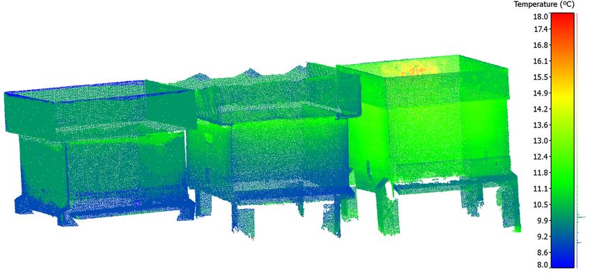
ISPRS Int. J. Geo-Inf. 2018, 7, 350                                                                2 of 16

regions. It is estimated that honeybees are responsible for 90–95% of all pollination carried out by
insects [20]. According to FAO (Food and Agriculture Organization of the United Nations), 71 of the
100 crop species which provide 90% of food worldwide are bee-pollinated. In Europe alone, 84% of
the 264 crop species are animal-pollinated and 4000 vegetable varieties exist thanks to pollination by
bees [21]. The production value of one metric ton of pollinator-dependent crop is approximately five
times higher than that of crop categories that do not depend on insects [22].
      It is therefore crucial to make beekeeping a more attractive hobby and a less laborious profession,
in order to encourage local apiculture and pollination. It is also essential to advance techniques that
allow non-invasive evaluation of colonies as this will minimize the human effect in the local ecosystem
and allow predictive decision making in maintenance tasks to ensure the survival of the largest number
of colonies possible.
      This work proposes and tests a methodology for the performance of the automatic assessment
of a honeybee hive population and the estimation of its growing state and survival capacities based
on the estimation and evaluation of the inner hive temperature extracted from data acquired with
different imaging sensors. The methodology consists of the processing and registration of visible
and thermographic images towards the generation of 4D temperature point clouds of hives, followed
by the computation and evaluation of the inner hive temperature via determination of the thermal
attenuation by conduction through the hive walls.
      The imaging sensors used for the objective of the paper are Red Green Blue (RGB) and thermal
cameras. RGB sensors are selected for the generation of accurate 3D models, while thermal cameras
are applied to the measurement of surface temperature in the bee hives. Although the latter can be
used for exploitation of the geometry of the object in the image [23], RGB cameras present a higher
resolution that enables the achievement of higher accuracy and resolution [24]. RGB and thermal data
fusion have been performed with different methodologies: From the registration image-to-image [25]
to registration RGB point cloud-to-image [26]. In both cases, knowledge of the inner orientation
parameters of the cameras is required, which is acquired through camera calibration. Camera
calibration has been widely studied for RGB cameras, with a variety of calibration fields in two
and three-dimensions [27,28], but also with algorithms for simultaneous calibration of the camera
while performing image orientation [29]. However, in the case of a thermal camera, the geometric
calibration is more complex due to the difficulty associated with these cameras when attempting to
distinguish between materials that are at the same temperature. For this reason, existing alternatives
for thermal camera geometric calibration are either based on temperature differences [30] or emissivity
differences [31].
      The paper has been structured as follows: After this introduction, Section 2 includes a detailed
explanation of the materials and methods used for data acquisition and processing. Section 3 deals
with an explanation of the methodology presented through its application to a real case study, based
on a set of honeybee hives selected as the case study; finally, Section 4 establishes the most relevant
conclusions of the approach proposed.

2. Materials and Methods

2.1. Equipment

2.1.1. RGB Camera
     A digital single-lens reflex (DSLR) camera was used to acquire images, as shown in Figure 1,
for the reconstruction of 3D point clouds, in addition to providing visual information of the state of
the hive walls. The visible camera selected for this work is a Canon EOS 700D (from Canon INC.,
Tokyo, Japan) equipped with a 60 mm fixed focal lens. This camera has a CMOS (Complementary
Metal-Oxide Semiconductor) sensor, which size is 22.3 mm × 14.9 mm. The size of the image captured
with this sensor is 18.5 MP with a pixel size of 4.3 µm.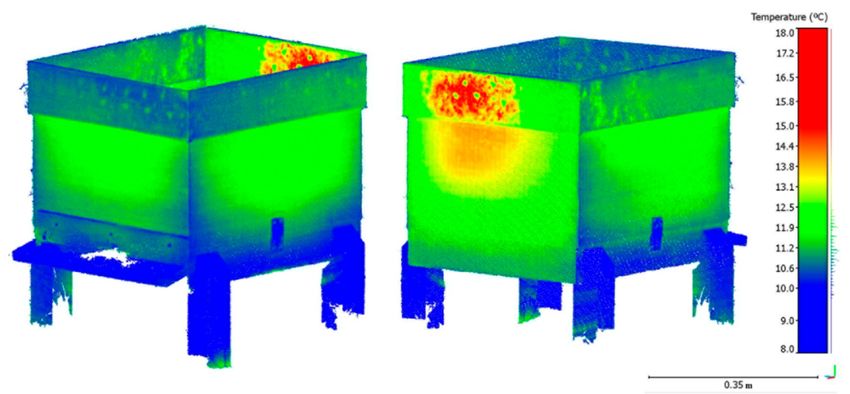
ISPRS Int. J. Geo-Inf. 2018, 7, 350 3 of 16
ISPRS Int. J. Geo‐Inf. 2018, 7, x FOR PEER REVIEW 3 of 15
Figure 1. Example of the images generated by the different imaging sensors used. (Left) Red Green
Figure 1. Example of the images generated by the different imaging sensors used. (Left) Red Green Blue
Blue (RGB) image. (Right) Example of the thermographic image acquired, with thermal values
(RGB) image. (Right) Example of the thermographic image acquired, with thermal values represented
represented using a color map: Dark blue is given to the lowest values (in this case, 2 °C), going to
using a color map: Dark blue is given to the lowest values (in this case, 2 ◦ C), going to light blue and
light blue and green for the highest temperature values (14 °C in this case study).
green for the highest temperature values (14 ◦ C in this case study).
The camera was calibrated prior to acquisition to allow for correction of the distortion and
The camera
perspective was
effects fromcalibrated prior to and
the data collected acquisition to allow for in
the 3D reconstruction correction of the distortion
the photogrammetric process.and
perspective
The camera effects from the
calibration data collected
working and the
in the visible band 3Dofreconstruction in the spectrum,
the electromagnetic photogrammetric
see Tableprocess.
1, is
The performed through theworking
camera calibration acquisition
in ofthemultiple
visible convergent
band of the images of a geometric
electromagnetic pattern (known
spectrum, as 1,
see Table
a calibration
is performed grid) with
through the different
acquisitionorientations
of multiple of convergent
the camera. images
The adjustment of the perspective
of a geometric pattern (knownrays as
governing the
a calibration position
grid) of the camera
with different and the image
orientations of the in each acquisition
camera. allows of
The adjustment forthe
theperspective
determination rays
of the inner
governing theorientation
position ofparameters
the cameraofand thethe
camera
image (focal length,
in each format size,
acquisition principal
allows for thepoint, and radial of
determination
thelens distortion;
inner in this
orientation case, the decentering
parameters of the camera of the lenslength,
(focal distortion is considered
format as negligible
size, principal point, given its
and radial
low value). The camera calibration was processed in the commercial photogrammetric
lens distortion; in this case, the decentering of the lens distortion is considered as negligible given station
its Photomodeler
low value). The Pro5© (by Photomodeler
camera calibration was Technologies,
processedVancouver, BC, Canada)
in the commercial which performsstation
photogrammetric the
automatic detection of the targets in each image, and computes and adjusts the orientation of each
Photomodeler Pro5© (by Photomodeler Technologies, Vancouver, BC, Canada) which performs the
image. This results in the computation of the internal calibration parameters of the camera and the
automatic detection of the targets in each image, and computes and adjusts the orientation of each
standard deviation of the calibration parameters as a value to test their quality [32].
image. This results in the computation of the internal calibration parameters of the camera and the
standard deviation
Table of orientation
1. Interior the calibration parameters
parameters of visibleascamera
a value to test
Canon EOStheir
700Dquality [32].
equipped with a 60 mm
fixed focal lens, as a result of its geometric calibration.
Table 1. Interior orientation parameters of visible camera Canon EOS 700D equipped with a 60 mm
Parameter
fixed focal lens, as a result of its geometric calibration. Value
Focal length, (mm) Value 64.214
Format size (mm × mm)
Parameter Value 24.746 × Value
15.164
Focal length, f (mm) X value
Value 11.392
64.214
Principal point (mm)
Format size (mm × mm) Y value
Value 7.736 × 15.164
24.746
Principal point (mm) KX value (mm−1)
1 value 9.498 ×11.392
10−6
Radial lens distortion
KY value (mm−3)
2 value 7.736
−3.350 × 10⁻⁸
K1 P1
value (mm −1 ) 9.498 ×−710−6
Radial lens distortion value (mm
−
−1) −1.772 × 10
Decentering lens distortion K2 value (mm 3 ) −1 −3.350 × 10⁻⁸
P2 value (mm ) 8.263 × 10⁻⁸ −7
P1 value (mm−1 ) −1.772 × 10
Decentering
Pointlens distortion
marking residuals Overall
P2 valueRMSE
(mm−1(pixels)
) 0.171
8.263 × 10⁻⁸
Point marking residuals Overall RMSE (pixels) 0.171
2.1.2. Thermal Data Acquisition
2.1.2. Thermal Data Acquisition
Thermographic data acquisition was performed with an NEC TH9260 camera, produced by
Nippon Avionics CO., see Figure 1, measuring temperatures ranging from −20 °C to 60 °C, with a
Thermographic data acquisition was performed with an NEC TH9260 camera, produced
thermal accuracy of 0.03 °C at 30 °C (30 Hz). Its sensor is an Uncooled Focal Plane Array (UFPA), 640
by Nippon Avionics CO., see Figure 1, measuring temperatures ranging from −20 ◦ C to 60 ◦ C,
× 480 (pixels) in size, capturing radiation between a wavelength of 7 μm and 14 μm.
with a thermal accuracy of 0.03 ◦ C at 30 ◦ C (30 Hz). Its sensor is an Uncooled Focal Plane Array
The main advantage of this camera for its use in the presented methodology is the availability
(UFPA), 640 × 480calibration,
of its geometric (pixels) in size, capturing
see Table radiation
2, so that between
its inner a wavelength
orientation ofare
parameters 7 µm and 14
known, µm.as
such
theThe main advantage
principal of this
point, sensor size,camera
and lensfordistortion
its use in coefficients.
the presented methodologycameras
Thermographic is the availability
capture
of radiation
its geometric
in the infrared range of the spectrum, in contrast to RGB (Red Green Blue)known,
calibration, see Table 2, so that its inner orientation parameters are camerassuch
that as
thework
principal point, sensor size, and lens distortion coefficients. Thermographic cameras
in the visible range. For this reason, the geometric calibration of the camera was performed capture
radiation in the infrared range of the spectrum, in contrast to RGB (Red Green Blue) cameras that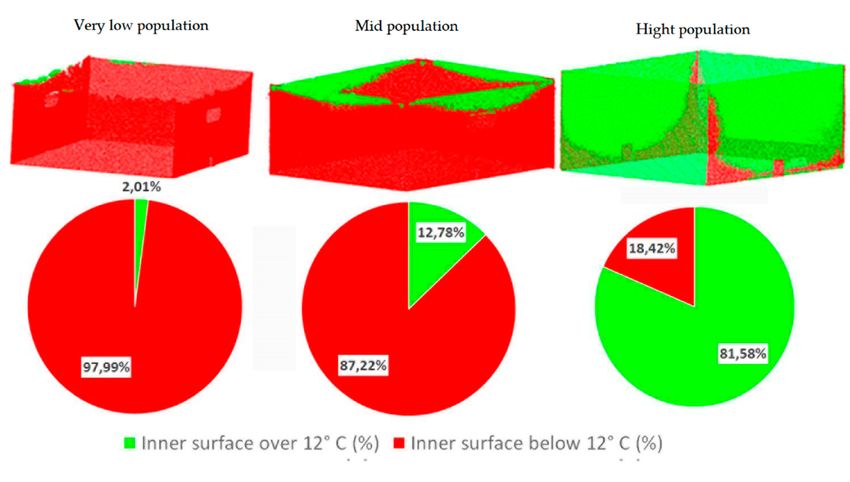
ISPRS Int. J. Geo-Inf. 2018, 7, 350                                                                   4 of 16

work in the visible range. For this reason, the geometric calibration of the camera was performed
using a specially designed calibration field, presented in [31], which is based on the capability of
the thermographic cameras to detect objects with different apparent temperatures even if they are
at the same real temperature, due to their different emissivity values. This calibration field consists
of a wooden plate with a black background (high emissivity) on which foil targets are placed (low
emissivity). In this case, the calibration was also processed in the commercial photogrammetric station
Photomodeler Pro5©.

      Table 2. Interior orientation parameters of thermographic camera, NEC TH9260, resulting from its
      geometric calibration.

                            Parameter                                                      Value
                     Focal length, f (mm)                     Value                       15.222
                   Format size (mm × mm)                      Value                   6.000 × 4.500
                                                             X value                       2.977
                      Principal point (mm)
                                                             Y value                      2.140
                                                         K1 value (mm−1 )             1.158 × 10⁻³
                     Radial lens distortion              K2 value (mm−3 )             −3.859 × 10⁻⁵
                                                         K3 value (mm−5 )             2.619 × 10⁻⁶
                                                         P1 value (mm−1 )             2.733 × 10⁻⁵
                  Decentering lens distortion
                                                         P2 value (mm−1 )             −2.413 × 10⁻⁵

     In addition to the thermographic camera, the acquisition of thermal data was complemented with
a contact thermometer, Testo 720, from Testo SE & Co. (Lenzkirch, Germany), see Table 3, used for
the measurement of the temperature of the honeybee hives in certain points to perform the emissivity
correction of each thermographic image. This way, all data needed for the thermographic analysis,
and for the emissivity correction of the values measured in the thermographic images, were available.

                                      Table 3. Thermometer, Testo 720, specifications.

                                      Parameter                     Value
                                        Range                  −50 ◦C  to 150 ◦ C
                                                         ±0.2 C (−25 ◦ C to +40 ◦ C)
                                                               ◦
                                                        ±0.3 ◦ C (+40.1 ◦ C to +80 ◦ C)
                                      Accuracy
                                                        ±0.4 ◦ C (+80.1 ◦ C to +125 ◦ C)
                                                        ±0.5 ◦ C (125 ◦ C)
                                      Resolution                    0.1 ◦ C

2.2. Methodology

2.2.1. Data Acquisition
     Proper data acquisition planning is important to optimize the resources available, ensuring the
high quality of the images and minimizing the capture time.
     Regarding the RGB sensor, the planning of data acquisition was carried out based on the classical
aerial photogrammetric principles [33] but adapted to the new algorithms and Structure from Motion
(SfM) strategies [34]. According to this, the scene must be exhaustively analyzed, since lighting
conditions are important as they determine the shooting strategy and the values of exposure, aperture,
and shutter speed of the camera. Thus, images should be acquired without illumination variations,
avoiding overexposed areas and ensuring sharpness. In addition, an analysis of possible occlusions
must be included, due to the probable presence of obstacles that will affect the protocol of multiple
image acquisition and the desired overlap percentage between adjacent images. Regarding the
geometric conditions of the photogrammetric data acquisition, the objective is to establish a multiple
image acquisition protocol to reconstruct the object or scene of interest, guaranteeing the highest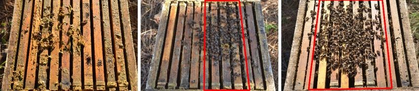
ISPRS Int. J. Geo-Inf. 2018, 7, 350 5 of 16
ISPRS Int. J. Geo‐Inf. 2018, 7, x FOR PEER REVIEW 5 of 15
highest completeness
completeness and accuracyand accuracy of the resulting
of the resulting 3D model. 3D model.
For thatFor that reason,
reason, the data theacquisition
data acquisition
must be
must be performed
performed followingfollowing some geometric
some geometric constraints.
constraints. In this In thisamong
case, case, among all possible
all possible trajectories
trajectories for the
for the camera to acquire images for the generation of a 3D model, a ring‐trajectory
camera to acquire images for the generation of a 3D model, a ring-trajectory around the object was around the object
was selected,
selected, as shown as shown in Figure
in Figure 2, maintaining
2, maintaining a constant
a constant distance
distance to the
to the object
object under
under study
study (depth)and
(depth)
and a specific
a specific separation
separation (baseline)
(baseline) between between
camera camera positions
positions or stations.
or stations. Regarding
Regarding the depth,
the depth, this
this should
should be chosen according to the image scale or the resolution desired. This theoretical
be chosen according to the image scale or the resolution desired. This theoretical definition of “scale” definition of
“scale” in digital close‐range photogrammetry is related to the geometric resolution
in digital close-range photogrammetry is related to the geometric resolution of the pixel size projected of the pixel size
projected over the object under study (Ground Sample Distance, GSD). This parameter can be
over the object under study (Ground Sample Distance, GSD). This parameter can be calculated by
calculated by considering the relationship between camera‐object distance, the GSD, the focal length
considering the relationship between camera-object distance, the GSD, the focal length of the sensor,
of the sensor, and the pixel size, as shown in Equation (1). Given the format difference between the
and the pixel size, as shown in Equation (1). Given the format difference between the thermographic
thermographic and RGB sensors, each camera‐object distance must be considered independently in
and RGB sensors, each camera-object distance must be considered independently in order to ensure
order to ensure a proper GSD.
a proper GSD.
f ps (1) (1)
=
D GSD
wheref is the
where is the focal
focal length
length of of
thethe sensor;
sensor; is the
D is the camera‐objectdistance,
camera-object distance,ps is isthethe size
size ofofthe
thepixel
pixeland
GSDandis the Ground
is the Ground
Sample Sample Distance.
Distance.
Regardingthethe
Regarding baseline,
baseline, avoiding
avoiding largelarge separations
separations between between
stationsstations
leads to leads
a high to a high
completeness
completeness of the 3D model due to the high image similarity and the
of the 3D model due to the high image similarity and the good image correspondences during thegood image correspondences
during
image the image phase.
orientation orientation phase. it
However, However, it is also necessary
is also necessary to consider to consider that baselines
that baselines that arethattooare
short
too short involve the computation of nearly parallel intersections between perspective rays, which
involve the computation of nearly parallel intersections between perspective rays, which can result in
can result in a worse accuracy of the resulting 3D point coordinates.
a worse accuracy of the resulting 3D point coordinates.
As shown in Figure 2, at least four stations of these “ring” acquisition protocols, denominated
As shown in Figure 2, at least four stations of these “ring” acquisition protocols, denominated as
as “master images”, are complemented with four images following a “mosaic” protocol; these latest
“master images”, are complemented with four images following a “mosaic” protocol; these latest are
are known as “slave images”. These slave images are taken by moving the camera slightly
known as “slave images”. These slave images are taken by moving the camera slightly horizontally
horizontally (left and right) and vertically (up and down) in relation to the master images, keeping a
(left and
high right) (80–90%).
overlap and vertically (up and down)
Complementary in relation
“master images”,to represented
the master images,
as blackkeeping
cameras ainhigh overlap
Figure 2,
(80–90%). Complementary “master images”, represented as black cameras in Figure
can be acquired with the aim of completing the geometry of the object under study, as established by 2, can be acquired
with the aim of completing the geometry of the object under study, as established by its complexity.
its complexity.
Figure2.2.“Master”
Figure “Master”and
and “slave”
“slave” images
images following
followingaa“ring”
“ring”ininthe
thedata
dataacquisition protocol.
acquisition protocol.
Regarding the thermographic sensor, there are several external parameters that influence the
Regarding the thermographic sensor, there are several external parameters that influence the
thermographic measurements, such as atmospheric attenuation, non‐uniform heating of the object
thermographic measurements, such as atmospheric attenuation, non-uniform heating of the object by
by solar incidence, and reflections produced by the radiation emitted and reflected by the
solar incidence,elements.
surrounding and reflections produced
The existence of by theinfluential
these radiation emitted and reflected
factors requires by the surrounding
the establishment of a
elements. The existence of these influential factors requires the establishment of a protocol for data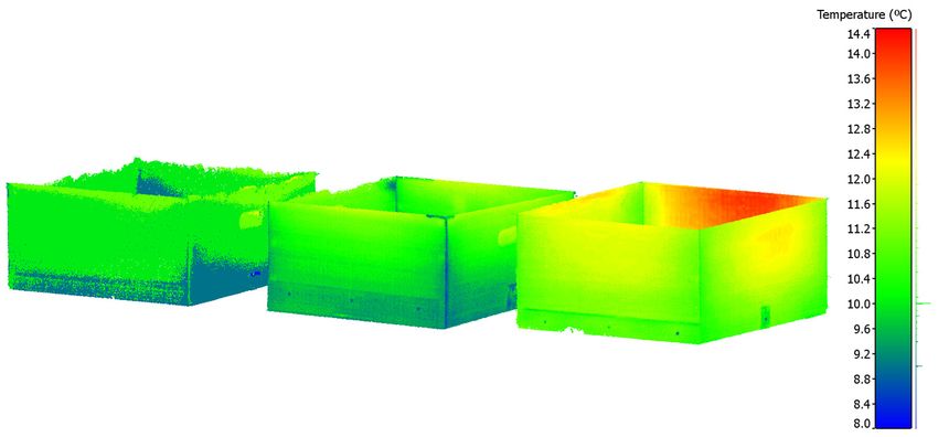
ISPRS Int. J. Geo-Inf. 2018, 7, 350                                                                6 of 16

acquisition with the aim of minimizing their effects and the acquisition of valid products for their
processing and analysis.
     The first rule is the adjustment of the ambient parameters in the camera for the atmospheric
correction; that is, the camera-object distance, ambient temperature, and humidity, prior to
data acquisition.
     The second rule is the acquisition of thermographic images with an angle of incidence of 20–25◦
between the normal of the object under study and the optical axis of the camera, avoiding the
measurement of radiation reflected from the operator and other surfaces.
     The third rule is the preparation of the data acquisition in order to achieve an approximate
steady-state heat transfer through the hive envelope conditions. For this reason, data acquisition
should be conducted at night after sunset or in the morning before sunrise, in order to minimize the
solar gain effect over the hive walls, with no wind and no precipitation events during the previous
48 h [35,36].
     Following these three rules, thermographic images were acquired in such a way that thermal
information was obtained for the totality of the surface of the object under study.

2.2.2. 3D Point Cloud Reconstruction
     The image-based modeling technique consisting of the combination of photogrammetry and
computer vision algorithms allows the reconstruction of dense 3D point clouds. This procedure is
preferably performed on the RGB images since their higher spatial resolution in comparison to the
thermographic images allows for more accurate results. It consists of two steps: Relative image
orientation and dense point matching for 3D point cloud generation. The procedure was performed
using GRAPHOS software, which is an integrated Photogrammetric Suite developed by the authors,
which allows dense and metric 3D point clouds from terrestrial and UAV (Unmanned Aerial Vehicle)
images to be obtained by enclosing robust photogrammetric and computer vision algorithms. More
information about GRAPHOS can be found in [37].
     The relative image orientation consists of the resolution of the spatial and angular position of the
camera and each image acquired in the 3D space. This process starts with the automatic extraction
and matching of image features through a variation of SIFT [38] (Scale-Invariant Feature Transform)
algorithm, called ASIFT [39] (Affine Scale-Invariant Feature Transform), which provides effectiveness
against other feature detection algorithms when considerable scale and rotation variations exist
between images. The homologous points detected through the ASIFT algorithm are the input for the
orientation and self-calibration procedure. The relative orientation is performed in two steps, first,
a pairwise orientation is executed by relating the images to each other by means of the Longuet-Higgins
algorithm [40] and second, this initial and relative approximation to the solution is used to perform
a global orientation adjustment between all images and a camera self-calibration by means of the
collinearity equations [41,42]. As a result, the spatial and angular positioning of the RGB sensor
was computed.
     The knowledge of the position of the RGB sensor in the acquisition of each image enables the
generation of a dense point cloud of the object under study (in this case, the beehive). In particular,
a dense matching method through the SURE (Photogrammetric Surface Reconstruction from Imagery)
implementation [43] based on the Semi-Global Matching technique (SGM) allows the generation of
a dense and scaled 3D point cloud resulting from the determination of the 3D coordinates of each pixel.
Regarding computational effort, the last step is the most expensive and time-consuming.
     With these steps, a dense 3D point cloud with RGB information was obtained for each case study.
The thermographic mapping of the 3D point cloud was solved manually through the identification
of homologous entities (interest points) between each thermographic image and the 3D point cloud.
This thermographic registration was obtained through the computation of the spatial resection [44]
of the thermographic images. As described in [45], the spatial resection makes use of image
coordinates and their homologous object coordinates to determine the position and orientation of the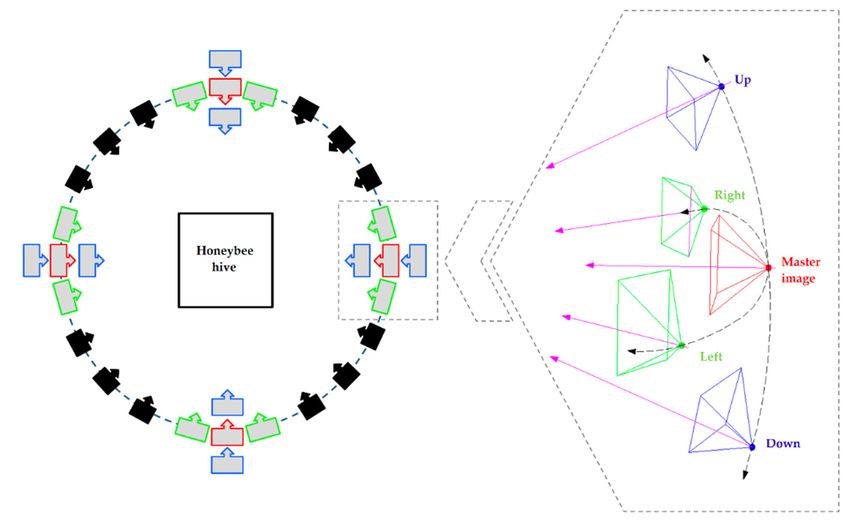
ISPRS Int. J. Geo-Inf. 2018, 7, 350 7 of 16
ISPRS Int. J. Geo‐Inf. 2018, 7, x FOR PEER REVIEW 7 of 15
thermographic camera in each image acquisition. Following this basic definition, spatial resection
ISPRS Int. J. Geo‐Inf. 2018, 7, x FOR PEER REVIEW 7 of 15
of
a single image can be extended to include the interior orientation parameters
a single image can be extended to include the interior orientation parameters of the imaging sensor, of the imaging sensor,
oraor
itsingle
can
it canbe reduced
image
be can be
reduced toto
include
includepositional
extended to includeelements
positional the interior
elements only (exterior
orientation
only orientation).
parameters
(exterior orientation). of the imaging sensor,
or itOnce
can the
be exterior
reduced to orientation
include of
positional each thermographic
elements only image
(exterior
Once the exterior orientation of each thermographic image is calculated, the is calculated,
orientation). thethermographic
thermographic
texture Once the exterior
transmitted to orientation
the 3D pointof each
cloud, thermographic
see Figure 3. image
The is
result calculated,
texture is transmitted to the 3D point cloud, see Figure The result obtained is a thermographic 4D4D
is obtained isthe
a thermographic
thermographic
texture
point
pointcloudis transmitted
cloud where
where each topoint
each the
point3D point cloud,
(X,Y,Z)
(X,Y,Z) has see Figure 3. value
hasaatemperature
temperature The result
value obtained is
(T)associated
(T) associated a thermographic
and
and represented
represented 4D
bybythethe
point
RGBRGB cloud
conversion where
conversion totoeach
the point (X,Y,Z)
thedefined
defined color has aMaximum
colormap.
map. temperature
Maximum value
and
and (T) associated
minimum
minimum temperatures
temperatures °C◦ C
and represented
ofof1818 by
and
and 8 ◦ C,
8the
°C,
RGB conversion
respectively,
respectively, were to
were the
selecteddefined
selected colortoto
ininorder
order map. Maximum
include
include the and
all the
all minimum
temperature
temperature temperatures
values
values presentedofand
presented 18
and°C and 8 °C,
optimize
optimize thethe
respectively,
representation
representation were
of of selected in order
temperaturevariations
temperature to include
variationswithin all
withinthe the temperature
the hives.
hives. values presented and optimize the
representation of temperature variations within the hives.
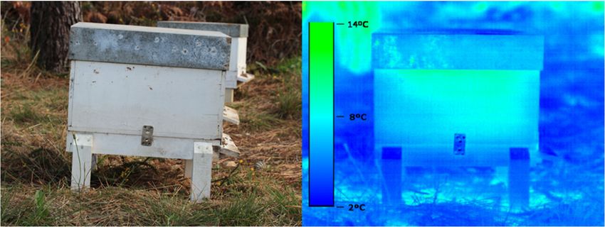
Figure 3. 4D point cloud with thermographic texture of one beehive. Front and right sides (Left). Back
Figure
Figure3.3.4D
4Dpoint
point cloud
cloud with
with thermographic textureofofone
thermographic texture onebeehive.
beehive.Front
Front and
and right
right sides
sides (Left).
(Left). Back
Back
and left sides (Right).
and left sides (Right).
and left sides (Right).
2.2.3. Estimation of Interior Honeybee Hive Temperature
2.2.3.
2.2.3.Estimation
EstimationofofInterior
Interior Honeybee
Honeybee HiveHive Temperature
Temperature
There are three different sources of infrared radiation captured by the thermographic camera if
weThere
Thereare
assume are three
that thedifferent
three different sources
sources
object under ofinfrared
of
study infrared
is radiation
radiation
opaque, captured
captured
implying that the by
the the thermographic
by transmission
thermographic cameracamera
if
of IR (InfraRed)
if we
we assume
assume that
that the
the object
object under
under study
study isis opaque,
opaque, implying
implying that
that thethe transmission
transmission of of
IR
radiation can be considered as null. These are the emissions from the object under study; the radiation IR (InfraRed)
(InfraRed)
radiation
radiation
reflected can
can bebeconsidered
from considered
the as null.
as
surroundingsnull. These
These
(both are
arethe
theemissions
attenuated emissions from
fromthe
by the atmospheric theobject
objectunder
under
transmission)study;
andthe
study; radiation
the
the radiation
emission
reflected
reflected
from the from
from thesurroundings
the
atmospheresurroundings
between the (both
(both attenuated
and theby
attenuated
camera by the
theatmospheric
object, as shown intransmission)
atmospheric transmission)
Figure 4. and thethe
and emission
emission
from
from thetheatmosphere
atmospherebetween
betweenthe the camera
camera and thethe object,
object,asasshown
shownininFigure
Figure4.4.
Figure 4. Components of incident InfraRed (IR) radiation acquired by the thermographic camera.
Figure 4.4.Components
Figure Components of
of incident
incident InfraRed
InfraRed(IR)
(IR)radiation
radiationacquired
acquiredbyby
the thermographic
the camera.
thermographic camera.
The emissivity correction is based on Stefan‐Boltzmann’s law [46,47], assuming that a real body
withThe emissivity
a surface correction
temperature is based by
measured on aStefan‐Boltzmann’s
thermometer can be law [46,47], assuming
considered that a real
as a real body, bodyit
whereas
The emissivity correction is based on Stefan-Boltzmann’s law [46,47], assuming that a real body
with
can abesurface temperature
considered measured
as a black by a thermometer
body when temperature can be considered
values are measured as a with
real body, whereas it
a thermographic
with
can
abe
surface temperature
considered
measured
as a black body when
by atemperature
thermometer can be considered
values are measured
as a real body, whereas
with a thermographic
camera (with no emissivity correction). This way, the emissivity correction is applied as Equation (2):
it camera
can be considered as a black body when temperature values are measured
(with no emissivity correction). This way, the emissivity correction is applied withasa Equation
thermographic
(2):
camera (with no emissivity correction). This way, the emissivity correction is applied as Equation (2) (2):
(2)
T4
where is the emissivity value for a real = rb
ε rb body,4
is the temperature measured with the(2)
where is the
thermographic emissivity
camera, and value fortemperature
is the a real body, Tbb
measuredis the temperature
by the measured with the
contact thermometer.
thermographic camera, and is the temperature measured by the contact thermometer.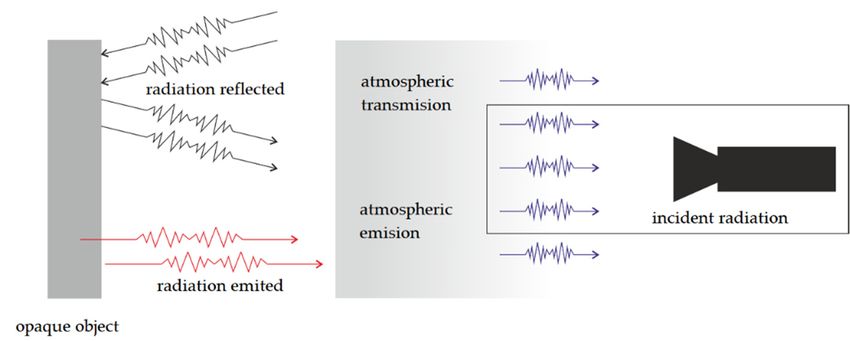
ISPRS Int. J. Geo-Inf. 2018, 7, 350 8 of 16
where ε rb is the emissivity value for a real body, Tbb is the temperature measured with the
thermographic camera, and Trb is the temperature measured by the contact thermometer.
ISPRS Int. J. Geo‐Inf.
In addition, the2018, 7, x FOR PEER
correction REVIEW
of the 8 of 15
atmospheric effect is directly performed by the thermographic
camera through the configuration of the ambient parameters (temperature and relative humidity) and
In addition, the correction of the atmospheric effect is directly performed by the thermographic
the camera-object distance.
camera through the configuration of the ambient parameters (temperature and relative humidity)
Assuming that the heat transfer through the hive wall is due to the conduction stream, while the
and the camera‐object distance.
heat transfer from the
Assuming thatouter
the heatparttransfer
of the hive wallthe
through to hive
the thermographic camera
wall is due to the combines
conduction convective
stream, while theand
radiant
heatstreams,
transfer fromsee Figure
the outer 5, part
which canhive
of the be explained with the following
wall to the thermographic cameraequations, Equationsand
combines convective (3)–(5):
radiant streams, see Figure 5, which can be explained with the following equations, Equations (3)–(5):
QCOND = U A( Tin − Twall ) (3)
(3)
QCONV = hout A( Twall − Tout ) (4)
(4)
4
Q RAD = 4εσATwall (5)
4 (5)
where QCOND , QCONV , and Q RAD are the conductive, convective, and radiant heat transfers (in W),
where , , and are the conductive, convective, and radiant heat transfers (in W),
respectively. U is the overall heat transfer coefficient for the beehive wall (W/m2 K),2 hout is the thermal
respectively. U is the overall heat transfer coefficient for the beehive wall (W/m K), is the
convective coefficient of the outer part of the beehive wall (W/m2 K), 2A is the area of the walls
thermal convective coefficient of the outer part of the beehive wall (W/m K), is the area of the
(discarding the area corresponding to the top cover, floor, and legs of the hive) where the heat transfer
walls (discarding the area corresponding to the top cover, floor, and legs of the hive) where the heat
takestransfer
place, takes
ε is the emissivity
place, is thevalue of thevalue
emissivity outerofsurface
the outerofsurface
the beehive
of the wall, andwall,
beehive σ isand
the Boltzmann
is the
constant, equal to 5.67 × 10 −8 W/m2 K4 [47]. T is the inner temperature of the hive, Twall is the
Boltzmann constant, equal to 5.67 × 10 W/m K4 [47].
−8 2 in is the inner temperature of the hive,
temperature of the exterior
is the temperature of thesurface of the
exterior beehive
surface wall,
of the in this wall,
beehive case measured
in this casein measured
the thermographies
in the
along all the beehivealong
thermographies surface and
all the Tout issurface
beehive the ambient
and temperature.
is the ambient temperature.
Figure
Figure 5. Diagram
5. Diagram of the
of the energy
energy balanceperformed
balance performed for
for the
the calculation
calculationofofthe inner
the temperature
inner of the
temperature of the
beehive: Heat flowing through the hive wall by conduction is equal to the heat exchanged from the
beehive: Heat flowing through the hive wall by conduction is equal to the heat exchanged from the
outer surface of the hive wall to the outer air by convection plus the heat exchanged by this surface
outer surface of the hive wall to the outer air by convection plus the heat exchanged by this surface by
by radiation; both sources of radiation were received by the thermographic camera.
radiation; both sources of radiation were received by the thermographic camera.
This total heat transfer from the exterior surface of the beehive wall to the thermographic camera
isThis total heat
assumed to betransfer
equal to from the exterior
the conduction surface
heat transferofthrough
the beehive wall
the hive to the
wall, thermographic
making camera
the assumption
that thermal
is assumed to beequilibrium
equal to theisconduction
obtained in heat
the hive, implying
transfer thatthe
through thehive
interior temperature
wall, making the is assumption
equal to
that the temperature
thermal of the interior
equilibrium surface
is obtained of the
in the wall.
hive, Consequently,
implying making
that the the temperature
interior heat flows equal [48], to
is equal
the inner temperature of the beehive wall can be calculated using Equation (6):
the temperature of the interior surface of the wall. Consequently, making the heat flows equal [48],
4
the inner temperature of the beehive wall can be calculated using Equation (6):
(6)
4
+ ,his
4εσTwall ( Twall − Tout )
The thermal convection outcalculated
Tincoefficient,
= according
+ Twallto [49] assuming horizontal (6)
heat flow through the beehive walls and naturalUconvection. The emissivity value, , for the outer
surface of the beehive wall is determined based on Stefan‐Boltzmann’s law [46,47] and the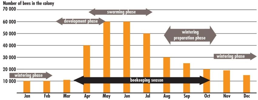
ISPRS Int. J. Geo-Inf. 2018, 7, 350 9 of 16
ISPRS Int. J. Geo‐Inf. 2018, 7, x FOR PEER REVIEW 9 of 15
temperature
The values and coefficient,
thermal convection are measured with the according
hout , is calculated thermographic
to [49] camera
assuming and the contact
horizontal
thermometer, see Equation (2).
heat flow through the beehive walls and natural convection. The emissivity value, ε, for the outer
surface of the beehive wall is determined based on Stefan-Boltzmann’s law [46,47] and the temperature
values Twall and
2.2.4. Geometric Tout are measured with the thermographic camera and the contact thermometer,
Preprocessing
see Equation (2).
Given that the result of the 3D reconstruction is an unordered high‐density point cloud with
2.2.4. Geometric
submillimetric GSDPreprocessing
and non‐uniform spatial distribution, it is necessary to apply a preprocessing
filter to normalize the 3D spatial
Given that the result of thedistribution of theis points.
3D reconstruction A Voxel‐Grid
an unordered subsampling
high-density point cloudalgorithm
with
implemented by PCL (Point Cloud Library) [50] was used to down‐sample the
submillimetric GSD and non-uniform spatial distribution, it is necessary to apply a preprocessing 3D point cloud
allowing
filterthe accurate evaluation
to normalize of the
the 3D spatial spatial distribution
distribution of the
of the points. points andsubsampling
A Voxel-Grid considerablyalgorithm
accelerating
the processing
implemented due to a (Point
by PCL significant
Cloud reduction
Library) [50]ofwas
theused
datato volume. These
down-sample thesubsampling
3D point cloudand filtering
allowing
the accurate
processes create aevaluation of the(aspatial
“Voxel grid” set of distribution
tiny 3D boxes of the points and
in space) overconsiderably accelerating
the input cloud the in
data. Then,
processing due to a significant reduction of the data volume. These subsampling and filtering
each voxel (i.e., 3D box) all the points will be approximated (i.e., downsampled) to their centroid. processes
create a “Voxel
This approach grid” (a
is slightly set of tiny
slower than3D boxes in space)them
approximating over the input
to the cloud
center ofdata. Then, in
the voxel, buteach voxel
it represents
(i.e., 3D box) all the points will be approximated (i.e., downsampled) to their centroid. This approach
the underlying surface more accurately. The result will be a homogeneous spatial distributed point
is slightly slower than approximating them to the center of the voxel, but it represents the underlying
cloud that allows the quantification of surfaces directly by counting points.
surface more accurately. The result will be a homogeneous spatial distributed point cloud that allows
the quantification of surfaces directly by counting points.
2.2.5. Honeybee Hive Population Assessment
2.2.5. Honeybee Hive Population Assessment
The AFSSET (French Agency for Environmental and Occupational Health Safety) describes in [51]
the meanThe AFSSET (French
theoretical honeybee Agency for Environmental
population per hive and and by
Occupational
season inHealth Safety)
temperate describes
regions, as in [51] in
shown
the mean theoretical honeybee population per hive and by season in temperate
Figure 6. Mortality is extremely high when activity is resumed at the end of winter and the beginning regions, as shown
in Figure
of spring 6. Mortality
coinciding with isthe
extremely
periodshigh whentemperatures,
of low activity is resumed
shortageat theofend of winter
food reserves,andandthe the
beginning of spring coinciding with the periods of low temperatures, shortage of food reserves, and
commencement of the use of chemicals in agriculture. During winter, the bees in the colony clump
the commencement of the use of chemicals in agriculture. During winter, the bees in the colony
together towards the middle of the hive, surrounding the queen. At this time, they allow the
clump together towards the middle of the hive, surrounding the queen. At this time, they allow the
temperature of the
temperature hivehive
of the to drop
to dropfrom
fromitsitsnormal
normal 3434 °C to around
◦ C to around2727◦ C°Cinside
inside
thethe cluster
cluster to conserve
to conserve
energy. Bees on the outer parts of the cluster, which will usually be around ◦9 °C,
energy. Bees on the outer parts of the cluster, which will usually be around 9 C, occasionally rotateoccasionally rotate
positions withwith
positions the the
beesbees
on on
thethe
more
morecrowded
crowdedinner
inner parts, sothat
parts, so thatallallthe
the bees
bees cancan keep
keep temperatures
temperatures
warmwarm
enough to survive.
enough Once
to survive. Oncethethedevelopment
developmentphase starts again,
phase starts again,the thepopulation
population of the
of the colony
colony is is
multiplied and and
multiplied the temperature
the temperatureof the inner
of the innerpart
partofofthe
thehive
hivewill
will raise backup
raise back about3434◦ C.
uptotoabout °C.
Figure 6. Mean
Figure theoretical
6. Mean honeybee
theoretical honeybeepopulation
population per hiveand
per hive andby
byseason
seasonin in temperate
temperate regions
regions (Source:
(Source:
UNEP UNEP
[3]). [3]).
Given the the
Given factsfacts
thatthat
thethe
survival
survivalofofthe
thecolony
colony is threatened
threatenedififthe
thetemperature
temperature cannot
cannot be kept
be kept
◦ C and the impossibility of each bee’s survival below 6 ◦
above 12 °C and the impossibility of each bee’s survival below 6 °C [52], the percentage of beehive
above 12 C [52], the percentage of beehive
wall wall surface
surface below,
below, between,
between, and
and overthese
over thesetemperature
temperature values
valuesisisused
used to to
evaluate the the
evaluate population
population
state of the colony. The segmentation of surfaces corresponding to the walls of the beehive was
performed through the implementation of a pass‐through filter. A pass‐through filter is a simple
filtering algorithm along a specified dimension cutting off values that are either inside or outside a
given user range.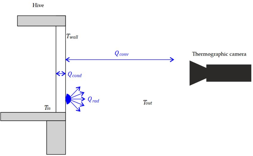
ISPRS Int. J. Geo-Inf. 2018, 7, 350 10 of 16
ISPRSstate
Int. J.of the colony.
Geo‐Inf. 2018, 7, xThe
FORsegmentation
PEER REVIEW of surfaces corresponding to the walls of the beehive was
10 of 15
performed through the implementation of a pass-through filter. A pass-through filter is a simple
filteringby
conducted algorithm
openingalong a specified
the top dimension
of the hive cuttingbetween
and looking off values that are
frames. eitherofinside
Some them or outside
will be found
a given user range.
to be populated by bees, while others are largely empty. Due to the impossibility of accurately
In order to compare results and validate the methodology, each representative hive was opened
quantifying the number of bees in a colony, the methodology used by some authors such as [53] was
to check their state at the moment of data acquisition. The process consists of a manual inspection,
applied, based on the correlation of the results with the frame count; referring to “frame count” as
conducted by opening the top of the hive and looking between frames. Some of them will be found to
the number of frames
be populated full
by bees, of bees,
while othersrounded toempty.
are largely the nearest
Due tointeger for each of
the impossibility hive body. quantifying
accurately
the number of bees in a colony, the methodology used by some authors such as [53] was applied, based
3. Experimental Results
on the correlation of the results with the frame count; referring to “frame count” as the number of
frames full of bees, rounded to the nearest integer for each hive body.
Study Case
3. Experimental Results
The proposed methodology was validated selecting three representative hives regarding their
Study Case
population (i.e., very low, normal, and high population with respect to the population values for each
phase, shown in Figures
The proposed 6–8); these
methodology was hives
validated were utilized
selecting forrepresentative
three the production
hives of honey their
regarding for self‐
consumption
populationand located
(i.e., in the
very low, town and
normal, of Castropol (Northern
high population withSpain)
respect(Latitude 43°31′ N, values
to the population Longitude
6°59′for
W).
eachThe first shown
phase, hive, shown on 6–8);
in Figures the left
theseinhives
bothwere Figures 7 and
utilized 8, was
for the chosenofdue
production to for
honey its low
population level. The
self-consumption andvisual
located inspection
in the town of carried
Castropolout(Northern
a few hours after the43◦imagery
Spain) (Latitude 310 N, Longitude
acquisition
6◦ 590 W).
confirmed theThe first hive, of
existence shown on the
a very left innumber
small both Figures 7 andpartially
of bees 8, was chosen due toonly
covering its lowone
population
frame. The
survival chances of colonies like this are very limited. In this case, all bees had disappearedthea few
level. The visual inspection carried out a few hours after the imagery acquisition confirmed
daysexistence
after theofdataa very small number
acquisition. The of bees partially
second covering
hive, shown onlymiddle
in the one frame.
imageThefeatured
survival inchances
Figures 7
of colonies like this are very limited. In this case, all bees had disappeared a few days after the
and 8, was selected as a representative for those hives where routine monitoring is necessary. Their
data acquisition. The second hive, shown in the middle image featured in Figures 7 and 8, was
population level is low, partially covering less than a half of the brood chamber stacks. If their
selected as a representative for those hives where routine monitoring is necessary. Their population
population level continues decreasing, maintenance tasks would be required to try to prevent the
level is low, partially covering less than a half of the brood chamber stacks. If their population level
extinction
continuesthe
of colony. maintenance
decreasing, The third hive,tasksshown
would on the righttointryFigures
be required 7 and
to prevent the 8, was selected
extinction of the as a
representation
colony. Theofthirdstrong colonies
hive, shown with
on thevery
righthigh populations.
in Figures 7 and 8,Inwas
thisselected
case, almost all frames are
as a representation offully
covered bycolonies
strong bees producing
with verylargehigh crowds at theIntop
populations. thisofcase,
the almost
stacks all
due to theare
frames high density
fully covered ofby
beesbeesinside
the hive. In this case, the hive does not need immediate attention, being able to face the wintering
producing large crowds at the top of the stacks due to the high density of bees inside the hive. In this
phasecase, the hive does not need immediate attention, being able to face the wintering phase successfully.
successfully.
Figure 7. Visual
Figure inspection
7. Visual from
inspection froma atop
topview
viewtoto determine thepopulation
determine the population through
through thethe count
count of frames
of frames
full of bees
full (highlighted
of bees in red).
(highlighted Very
in red). Verylowlowlevel
levelof
of population (Left).Mid
population (Left). Mid level
level of of population
population (Middle).
(Middle).
HighHigh
levellevel
of population (Right).
of population (Right).Figure 7. Visual inspection from a top view to determine the population through the count of frames
ISPRS full
Int. of bees (highlighted
J. Geo-Inf. 2018, 7, 350 in red). Very low level of population (Left). Mid level of population (Middle).
11 of 16
High level of population (Right).
Figure 8.
Figure 8. 4D models which
4D models which integrate
integrate metric
metric and thermographic information.
and thermographic information. Very low level
Very low level of
of
population (Left). Mid level of population (Middle). High level of population (Right).
population (Left). Mid level of population (Middle). High level of population (Right).
Data acquisition was performed in November, immediately after honey gathering works and the
preparation of hives for the start of the wintering phase. This preparation consists of the removal of all
supplementary stacks keeping only the “brood chamber” (bottom stack). Each frame of the “brood
chamber” was examined in order to ensure that all hives have some stacks with breeding and the
remaining are full of honey, ensuring the existence of food for the survival of the hive until the next
beekeeping season.
Data acquisition was carried out in the morning before sunrise. The ambient temperature at the
time of data acquisition was 10 ◦ C.
Data acquisition was planned independently for each sensor according to the directives described
in Section 2.2.1. Considering that the objective of this step is to achieve a high-resolution 4D point
cloud, the GSD was fixed to 1 mm for the RGB sensor and 5 mm for the thermographic sensor allowing
the performance of image acquisition at a distance from the hive of up to 14 m and 2 m, respectively.
The RGB images were processed according to the photogrammetric and computer vision
methodologies described in Section 2.2.2, obtaining a point cloud of each hive with an average
resolution of more than 1,000,000 points/m2 . The geometric accuracy of the reconstructed 3D RGB
cloud was validated by comparing the main dimensions of the hives (i.e., width, height, and diagonals
of each hive face) between the reconstructed 3D RGB cloud and the real hive. As a result, an
averaged deviation of 3.5 mm with a maximum deviation of 5 mm was obtained. In addition,
point-to-plane deviations were used to validate the reconstruction noise. Assuming that each hive
face is a perfect plane, the least squares algorithm was used to compute and analyze point-to-plane
deviations. These deviations present a normal distribution over the surface of the hive, with a mean
of 0.8 mm and a standard deviation of 1.3 mm. The thermographic texture was projected over the
point cloud obtaining a hybrid 4D point cloud with thermographic texture mapped over the points of
the hive.
This 4D point cloud with thermographic texture is subjected to a manual segmentation process to
remove those parts that are not of interest, such as the top cover, floor, legs, or surrounding elements
that do not belong to the hive, as shown in Figure 9.of 0.8 mm and a standard deviation of 1.3 mm. The thermographic texture was projected over the
point cloud obtaining a hybrid 4D point cloud with thermographic texture mapped over the points
of the hive.
This 4D point cloud with thermographic texture is subjected to a manual segmentation process
to Int.
ISPRS remove those
J. Geo-Inf. parts
2018, 7, 350that are not of interest, such as the top cover, floor, legs, or surrounding
12 of 16
elements that do not belong to the hive, as shown in Figure 9.
Figure
Figure 9. Segmentationofofthe
9. Segmentation thehives:
hives:Surfaces
Surfaces to
to be
be evaluated
evaluated of
ofthe
thethree
threehives
hivesfor
fortheir
theirpopulation
population
assessment. Very low level of population (Left). Mid level of population (Middle).High
assessment. Very low level of population (Left). Mid level of population (Middle). High level of of
level
population (Right).
population (Right).
The inner temperature of the hive was calculated at each 3D point. To this end, information
The the
about inner temperature
material of the hive
and thickness of thewas
hivecalculated
walls was at required,
each 3D point.
as shownTo this end, information
in Equation about
(6). A digital
thesuperficial
material and thickness of
thermometer the hive
(Testo 720)walls was required,
was used to measure as shown in Equation
the interior temperature(6). Aatdigital
certainsuperficial
points
thermometer (Testo 720) was used to measure the interior temperature
inside the hive. The comparison of the thermal values of the camera and the contact thermometer at certain points inside the
hive.
wereThe comparison
inside of the thermal
the confidence interval values
definedof bythe thecamera
contactand the contact
thermometer thermometer
manufacturer of were
±0.2°.inside
So,
thethe
confidence
confidence interval
level ofdefined by the
the results contactby
is limited thermometer
the accuracymanufacturer
of the contact of ±0.2◦ . So, the
thermometer. confidence
In this case,
level
hiveofwalls
the results
were built is limited
with wood by the
withaccuracy
a thermalofconductivity
the contactUthermometer.
of 0.13 m K/W and In this case, hive
a thickness walls
of 0.03
ISPRS Int. J. Geo‐Inf. 2018, 7, x FOR PEER REVIEW 12 of 15
were built with wood with a thermal conductivity U of 0.13 m K/W and a thickness of 0.03 m. Hive
walls are topped
m. Hive walls are with a thin
topped withlayer of paint;
a thin layer ofhowever, the effect
paint; however, theof the paint
effect of the onpainttheoncalculation
the calculationcan be
dismissed due to its negligible thickness and to the fact that it would only
can be dismissed due to its negligible thickness and to the fact that it would only affect the emissivity affect the emissivity value
of value
the surface.
of the surface.
TheThe4D4D model
modelwith withthermal
thermalinformation
information of the interior
interiorof ofthe
thehive
hiveisissubjected
subjected toto a pass-through
a pass‐through
filter to evaluate the surface in the
filter to evaluate the surface in the hive interior hive interior that is over 12 ◦
°C, see Figure 10.
is over 12 C, see Figure 10. A normal A normal behavior
behavior
of of
thethe temperaturedistribution
temperature distributionon onthe
the inner
inner surface
surface of of the
the hive
hivecan canbebeseen.
seen.Following
Following thethe
upward
upward
flow
flow of of
hothot air,
air, thethesurface
surfacetemperature
temperatureis is higher
higher in in the
the upper
upperareaareaofofthe
thestack.
stack.AA direct
directrelationship
relationship
between
between theinner
the innersurface
surfaceof ofthethehive
hive walls
walls that
that thethe colony
colonyisisable
abletotomaintain
maintainabove above 1212 °C◦ and
C and thethe
population density
population density can be seen. can be seen.
Figure
Figure10.10.Surface
Surfaceevaluation
evaluationover
overpass-through filter results.
pass‐through filter results.Very
Verylow
lowlevel
levelofofpopulation
population (Left).
(Left). Mid
Mid
level of of
level population
population(Middle).
(Middle).High
Highlevel
level of
of population (Right).
population (Right).
4. Conclusions
This article presents a non‐invasive methodology for the analysis of the population condition
and growing capabilities of honeybee hives through the generation of 4D models with geometric
(X,Y,Z) and inner temperature (T) information. An automatic process for the analysis of the survival
options of colonies for the wintering phase based on the evaluation of the colony capability toYou can also read