Explaining the Past and Projecting Future Crime Rates James Austin, Todd Clear, and Richard Rosenfeld - HARRY FRANK GUGGENHEIM FOUNDATION
←
→
Page content transcription
If your browser does not render page correctly, please read the page content below
Explaining the Past and
HARRY FR ANK        Projecting Future Crime Rates
GU GG EN H EI M
F O U N DAT I O N

                    James Austin, Todd Clear,
                    and Richard Rosenfeld
Explaining the Past and
HARRY FR ANK        Projecting Future Crime Rates
GU GG EN H EI M
F O U N DAT I O N

                    James Austin, Todd Clear,
                    and Richard Rosenfeld

                    September 2020

                    120 West 45th Street   T 646.428.0971
                    New York, NY 10036     www.hfg.org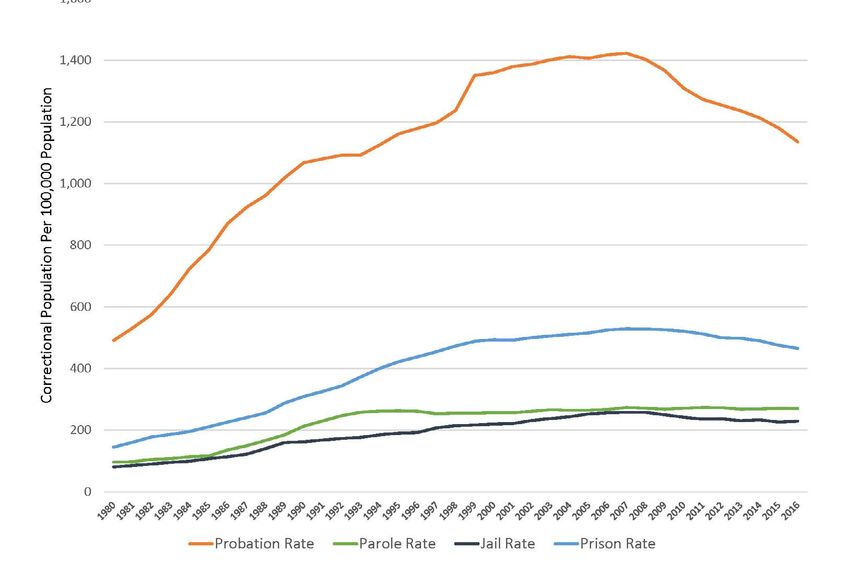
Abstract

To date criminologists have a poor record of anticipating future
crime rates. As a result, they are ill-equipped to inform policy makers
about the impact of criminal justice reforms on future crime. In this
report, we assess the factors that explain changes in crime during the
past three decades. Our analysis shows that macro-level economic and
demographic factors best explain trends in violent and property
crime. Together, those factors outweigh the impact of imprisonment
rates on crime. We also show that it is possible to lower imprisonment
rates without causing an increase in crime. Indeed, several states have
done exactly that. Finally, we present models for projecting future
crime rates. Based on these models, crime is projected to decrease over
the next five years. The next step should be to apply similar analyses to
individual states and local jurisdictions to advise policy makers on the
implications of their criminal justice reform strategies for public safety.
Introduction
Major changes in America’s crime rates have occurred since the mid-1960s. After several decades
of relative stability, a significant unanticipated uptick in crime began in 1965, reaching historic
peaks in the early 1980s and then again in the early 1990s. During this period crime rates more
than tripled. However, suddenly and just as unexpectedly, crime then began to decline rapidly,
reaching its lowest level since 1966 (Figure 1). Today, it is unclear whether crime rates will continue
to decline, stabilize, or begin to increase. Most research to date on understanding crime rates in
the United States and elsewhere has been limited to identifying factors that are associated with
past crime rates (Rosenfeld 2011). Much less attention has been devoted to projecting future
crime rates.
There are several problems with these studies of changes in crime rates. First, criminologists have
been unable to develop statistical models that would have predicted the sudden rise and fall in
crime. While accounting for past crime trends is an important exercise, of greater value to society
and policy makers would be methods for projecting future crime rates based on assumptions
about a small set of key factors, some modifiable through policy and some not, that research has
shown to have influenced crime trends.
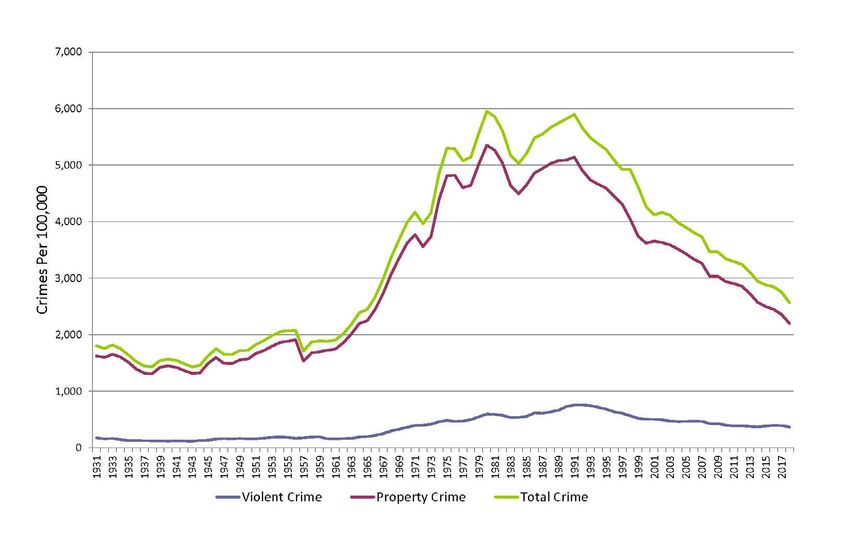
F I G U R E 1. U C R C R I M E R AT E S , 1931–1981
1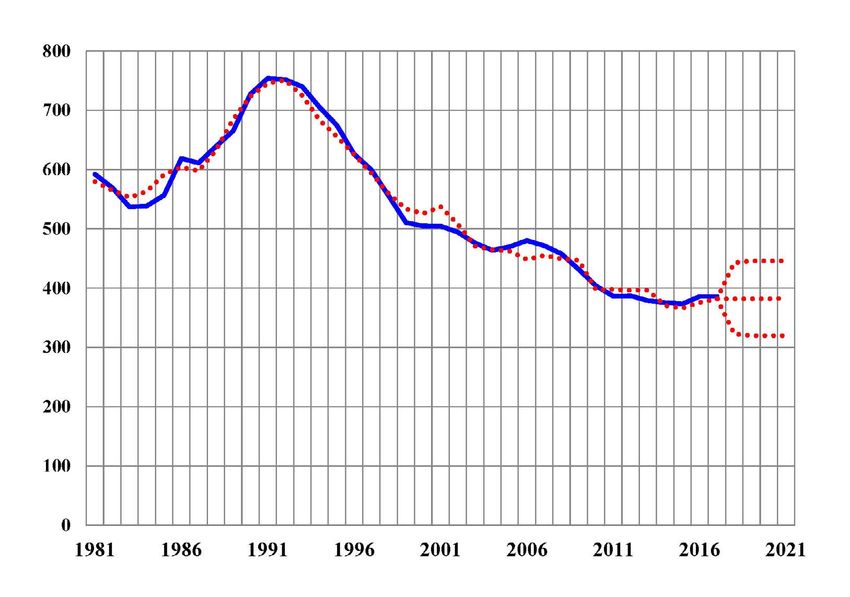
Second, these studies have not paid sufficient attention to macro-level economic factors such as
inflation rates and consumer confidence and socio-demographic factors (e.g., fertility rates,
household size) that hold some promise for projecting crime rates into the future (Rosenfeld and
Levin 2016).

Third, such models have narrowly tried to factor in the impact of the criminal justice system
(e.g., incarceration rates, size of police forces) to estimate what changes in criminal justice policy
can serve to increase or decrease crime rates. For example, Levitt (2004) argues that increases in
the size of city police forces contributed to the sustained U.S. crime drop that began in the early
1990s. Conversely, Sharkey, Torrats-Espinosa, and Takya (2017) found that the increased presence
of community-based organizations in high crime neighborhoods reduces crime rates and may
have supplanted the impact of law enforcement in such communities.

Fourth, on the incarceration side, most studies have claimed that the higher imprisonment rates
that began in the 1970s were at least partially responsible for the subsequent reductions in crime
that began in the early 1990s (e.g., Levitt 1996, 2004). These studies focus on imprisonment
rates as the sole criminal-justice variable, however, and ignore the three other major forms of
correctional control: probation, parole, and jails. When the effects of these other forms of
correctional control are added to any statistical model, the impact of state imprisonment rates
cannot be reliably estimated because, as we will show, all four forms of correctional control are
highly interrelated.

In addition, rising imprisonment rates seem to have “diminishing returns” for crime reduction
(Gainsborough and Mauer 2000; Stemen 2007). At least one study found that, after a certain point,
increased imprisonment rates may actually increase crime (Vieraitis, Kovandzic, and Marvell 2007).

The impact of incarceration policy (both jails and prison) on crime is particularly relevant today
as state and local governments are being urged to lower their jail and prison populations. Policy-
makers need confidence that reductions in their correctional populations will not increase their
crime rates. Forecasting models in criminal justice have been largely limited to estimating the
impact of sentencing reforms and administrative policies (e.g., parole-board grant rates, good-
time-credit awards) on the size of correctional populations. Efforts to estimate the impact of
such reforms on crime rates are almost non-existent. A recent exception is a study commissioned
by the state of Illinois on how to safely reduce its prison population by 25%, which showed that
such a reduction could be achieved without increasing crime (Austin et al. 2017).

2
A Primer on Crime Rates and Crime Trends

There are two methods for measuring crime in the United States. The longest-standing method
is through the FBI’s Uniform Crime Reports (UCR), which has been collecting data since 1931.
The UCR is based only on incidents of the following crimes reported to and recorded by the police:

   1.   Murder
   2.   Rape
   3.   Robbery
   4.   Aggravated Assault
   5.   Burglary
   6.   Larceny
   7.   Auto Theft
   8.   Arson

The UCR crime rate is expressed as crimes per 100,000 U.S. population as reported by the
U.S. Census. The conventional use of a rate using large numbers—crimes per 100,000—tends
to obscure the fact that the risk of being victimized by a serious crime is low. For example,
the 2017 crime rate was 2,756 per 100,000, which means that only 2.7% of the U.S. population
reported experiencing one of the eight UCR crimes recorded by police that year (or less if some
persons reported more than one crime).

Several major trends shown in Figure 1 should be emphasized. First, rates were relatively stable
and low (under 2,000 per 100,000) from 1931 until the 1960s, when they began to rise, reaching
a peak of 6,000 per 100,000 by the early 1980s. While this represents a three-fold increase in
the crime rate, it also means that at its highest peak, at most 6% of the U.S. population reported a
serious crime to police each year.

Second, the vast majority (about 85% of the total crime rate) of UCR crimes are non-violent
offenses, mainly larceny theft (about 60% of the total). The violent crime rate (mostly aggravated
assault and robbery) peaked in 1991 at 758 per 100,000, meaning that, at its highest point, only
eight-tenths of one percent of the U.S. population reported a violent crime to police.

Finally, as mentioned, after a dramatic rise that began in the early 1960s and peaked in the early
1980s and again in the early 1990s, the UCR rates have steadily declined since the early 1990s.
As of 2017, they had declined to the rates of 1966.

                                                                                                   3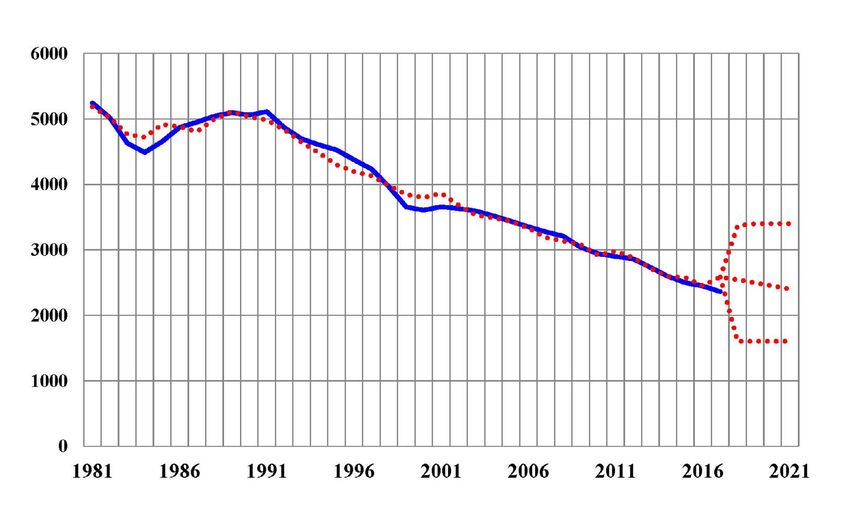
A major benefit of the UCR is that it allows local jurisdictions to measure their own crime
rate and compare it with others. But because the data reflect incidents reported to and recorded
as crimes by the police, they do not include crimes unknown to the police. To correct for this
limitation, the Bureau of Justice Statistics of the U.S. Department of Justice began a new crime
reporting program in 1973 that is based on a national survey of U.S. households. Known now
as the National Crime Victimization Survey (NCVS), this survey counts all crimes against
members of the sampled household who are 12 years or older.1

There are important differences and similarities between the extent of crime as measured by the
UCR and the NCVS. The NCVS does not include homicide. UCR rates are lower than NCVS
rates because many crimes, especially minor ones, are not reported to police. A major reason for
the lower numbers in the UCR is that many of the crimes reported in the NCVS involve little to
no economic loss or injury and are thus less likely to motivate victims to report them to police.

                                                    F I G U R E 2 . N C V S R AT E S , 198 0 –2 018

1 B E C A U S E I T I S A N AT I O N A L S U R V E Y, I T I S N OT P O S S I B L E TO M E A S U R E C R I M E R AT E S F O R LO C A L J U R I S D I C T I O N S A N D S TAT E S . T H E
  B U R E A U O F J U S T I C E S TAT I S T I C S I S C U R R E N T LY D E V E LO P I N G M E T H O D S TO E S T I M AT E S TAT E - L E V E L V I C T I M I Z AT I O N R AT E S .

4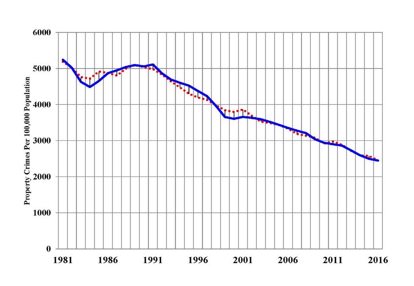
Despite these differences, the NCVS shows the same downward trajectory as the UCR data since
the early 1980s and, for violent crime, the early 1990s (Figure 2). And the same lessons emerge:
the annual probability of a U.S. resident being a victim of any crime is low—extremely low for
a violent crime—and victimization risk has dropped dramatically since the early 1990s. For
example, the probability of being victimized for a violent crime as measured by the UCR is now
only four-tenths of one percent. For property crime (burglaries, larcenies, and motor vehicle
thefts) the risk is now 2.5%.

The NCVS shows that the probability of being victimized for a serious violent crime (aggravated
assaults, robberies, and rapes) each year is now six-tenths of one percent for the population age
12 and older. The chance that a household will be victimized by a burglary or auto theft is
now 2.7%. In short, the chance of being a victim of a crime documented by the UCR or NCVS
is lower than at any point during the past half century. It goes without saying that criminologists
failed to anticipate both the rapid ascent and equally dramatic decline in crime rates of the
past several decades. The factors that have driven crime to such low levels and whether these
downward trends will continue are the subject of the remainder of the report.

                                                                                                 5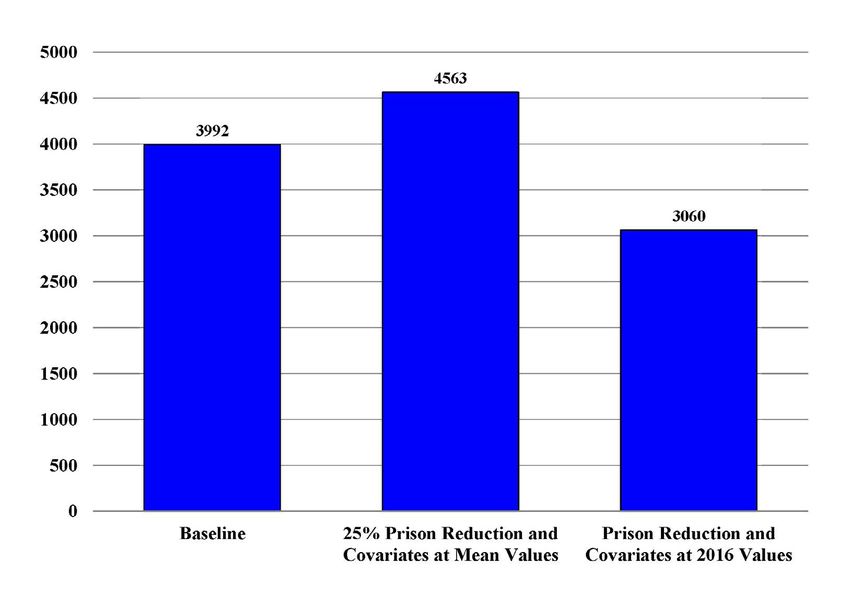
Explaining the Fall in U.S. Crime Rates

To explain why U.S. crime rates have declined so rapidly, we gathered national data on variables
that, based on past research, might have influenced national crime rates (both UCR and NCVS)
during our study period, 1980 to 2016. The variables include demographic, social, and economic
conditions, as well as state and federal imprisonment rates. We also collected data on the other
portions of the U.S. correctional population – probation, jail, and parole populations. We do not
include these correctional indicators in our statistical analyses, however, because, as mentioned,
it is very difficult to distinguish the impact of the prison population on crime rates from that of
probation, jail, and parole.

Any statistical model of crime rates is intended to explain why rates change from year to year.
This is typically accomplished with a multiple-regression statistical analysis. Such a quantitative
model is able to estimate the independent effect of each of a number of variables.

Our objective was to develop regression models with the strongest fit to the year-to-year variation
in violent and property crime rates between 1980 and 2016. We do not attempt to explain why
the UCR crime rates began to rise in the mid 1960s until they plateaued in 1980. This is because
many of the variables we examine are not readily available prior to 1980. And the NCVS, which
is considered to be a more comprehensive reading of crime, did not exist prior to 1973.

The national-level analyses we conducted are meant to provide guidance to policymakers in
estimating the impact on crime of reforms intended to reduce correctional populations. But
criminal justice policy is enacted primarily at the state and local level. To be of practical utility,
such analyses should be carried out using data for states, counties, and cities. The specific
conditions that affect crime rates in these jurisdictions may differ from those associated with
national-level crime rates. The national-level analyses illustrate the logic and methods that should
inform comparable analyses carried out at lower geographic levels. We present preliminary
state-level analyses of the impact of imprisonment levels on crime rates later in this report.

We carried out the national-level analyses using the UCR violent and property crime rates; prior
research on crime and imprisonment trends has almost exclusively been based on the UCR data.2

2 W E R E P L I C AT E D T H E S E A N A LY S E S O N N C V S V I O L E N T A N D P R O P E R T Y C R I M E T R E N D S O V E R T H E S A M E P E R I O D. T H E M O D E L
  S P E C I F I C AT I O N S D I F F E R E D S O M E W H AT. O V E R A L L , H O W E V E R , T H E R E S U LT S W E R E S I M I L A R T O T H O S E B A S E D O N T H E U C R
  C R I M E D ATA R E P O R T E D H E R E .

6
The best-fitting model for explaining the UCR violent crime trends (Figure 3) consisted of five
factors: the inflation rate, the teen birth rate, the divorce rate, the percentage of the population
between the ages of 18 and 24, and the imprisonment rate (state plus federal). Past research
has shown that these measures are significantly associated with changes in violent crime rates
(e.g., Colen, Ramey, and Browning 2016; Rosenfeld and Levin 2016; Travis, Western, and
Redburn 2014:146-150).3 The inflation, teen birth, and divorce rates are positively associated
with the violent crime rate (Table 1). (As inflation, teen birth, and divorce rates increase, the
violent crime rate increases; as they decrease, the violent crime rate decreases.) The percentage
of the population between 18 and 24 is negatively related to the violent crime rate.4
TA B L E 1. FAC T O R S A S S O C I AT E D W I T H U C R
V I O L E N T C R I M E R AT E , 198 0 -2 016
Factor b-Slope Standard Error
Inflation Rate (lagged) 5.344* 1.934
Teen Birth Rate (lagged) 10.115* .929
Divorce Rate (lagged) 72.514* 18.647
% 18–24 −93.616* 19.155
State and Federal Imprisonment (lagged) −1.498* .156
R Square (Variance Explained) 98%
Without State and Federal Imprisonment Rate 77%
F-Test of Overall Significance 173.2*
*P < .01
N OT E : P R A I S - W I N S T E N R E G R E S S I O N . I N D E P E N D E N T VA R I A B L E S , E XC E P T %18 - 24 , A R E L A G G E D O N E Y E A R .
VA R I A B L E D E F I N I T I O N S
V I O L E N T C R I M E R AT E = S U M O F U C R H O M I C I D E S , R A P E S , R O B B E R I E S ,
A N D A G G R AVAT E D A S S A U LT S P E R 10 0 , 0 0 0 P O P U L AT I O N
I M P R I S O N M E N T = S TAT E A N D F E D E R A L P R I S O N E R S P E R 10 0 , 0 0 0 P O P U L AT I O N
I N F L AT I O N = Y E A R LY P E R C E N TA G E C H A N G E I N C O N S U M E R P R I C E S
T E E N B I R T H R AT E = B I R T H S P E R 1, 0 0 0 F E M A L E S A G E 15 -19
D I V O R C E R AT E = P E R C E N TA G E O F T H E P O P U L AT I O N A G E 15 A N D O L D E R D I V O R C E D
% 18 - 24 = P E R C E N TA G E O F T H E P O P U L AT I O N B E T W E E N 18 A N D 24 Y E A R S - O L D
3 TO C O R R E C T T H E E S T I M AT E S F O R A U TO C O R R E L AT I O N , W E E S T I M AT E D T H E M O D E L S W I T H P R A I S - W I N S T E N ( A R 1) R E G R E S S I O N .
4 A S T H E F R A C T I O N O F T H E P O P U L AT I O N I N T H E 18 - 24 S E G M E N T H A S FA L L E N , W E M I G H T H AV E E X P E C T E D T H E V I O L E N T C R I M E R AT E
TO D E C R E A S E , B E C A U S E O F F E N D I N G T E N D S TO P E A K D U R I N G YO U N G A D U LT H O O D. H O W E V E R , F O R T H E P E R I O D O F O U R S T U DY,
19 8 0 - 2 0 16 , W E F O U N D A N E G AT I V E R E L AT I O N S H I P. A P R O B A B L E E X P L A N AT I O N I S T H AT T H E R AT E O F Y O U T H V I O L E N C E S H O T U P
D U R I N G T H E C R AC K ER A O F T H E L AT E 198 0 S A N D E A R LY 19 9 0 S , E V EN A S T H E YO U T H F U L CO H O R T O F T H E P O PU L AT I O N WA S S H R I N K I N G
( C O O K A N D L A U B 19 9 8 ) . T H E C O R R E L AT I O N B E T W E E N T H E P E R C E N TA G E O F T H E P O P U L AT I O N B E T W E E N 18 A N D 24 A N D T H E
V I O L E N T C R I M E R AT E WA S T H U S S T R O N G LY N E G AT I V E D U R I N G T H E 19 8 6 -19 9 2 C R A C K E R A . E V E N T H O U G H T H E R E L AT I O N S H I P WA S
P O S I T I V E B OT H B E F O R E A N D A F T E R T H AT B R I E F P E R I O D, T H E N E T R E L AT I O N S H I P O V E R T H E 19 8 0 - 2 016 P E R I O D WA S N E G AT I V E .
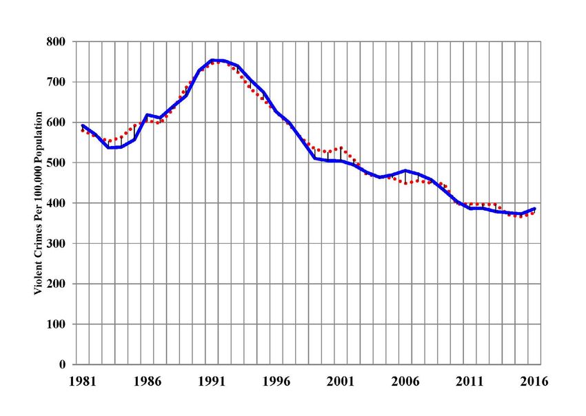
7F I G U R E 3 . O B S E R V E D A N D PR E D I C T E D
V I O L E N T C R I M E R AT E , 1981–2 016
PREDICTED
OBSERVED
R 2 = 0 .9 8 2
F I G U R E 4 . O B S E R V E D A N D PR E D I C T E D
PRO PE R T Y C R I M E R AT E , 1981–2 016
OBSERVED
PREDICTED
R 2 = 0 .9 8 4With regard to UCR property crime rates (burglaries, larcenies, and motor vehicle thefts per
100,000 population) (Figure 4), the best-fitting model includes the inflation rate, the percentage
of the population between 18 and 24, the percentage of the labor force in manufacturing jobs,
and a measure of educational attainment—the percentage of the population age 25 and older
with a bachelor’s or higher degree (Table 2).
TA B L E 2 . FAC T O R S A S S O C I AT E D W I T H U C R
PRO PE R T Y C R I M E R AT E , 198 0 -2 016
Factor b-Slope Standard Error
Inflation Rate (lagged) 58.427* 12.086
% Bachelor's or Higher Degree −356.858* 56.207
Proportion in Manufacturing −25326.330* 8599.319
% 18–24 −675.997* 112.063
State and Federal Imprisonment (lagged) −6.439* 1.409
R Square (Variance Explained) 98%
Without State and Federal Imprisonment Rate 93%
F-Test of Overall Significance 238.3*
*P < .01
N OT E : P R A I S - W I N S T E N R E G R E S S I O N
VA R I A B L E D E F I N I T I O N S
P R O P E R T Y C R I M E R AT E = S U M O F U C R B U R G L A R I E S , L A R C E N I E S , A N D M OTO R V E H I C L E
T H E F T S P E R 10 0 , 0 0 0 P O P U L AT I O N
% B A C H E LO R ’ S O R H I G H E R D E G R E E = P E R C E N TA G E O F T H E P O P U L AT I O N A G E 2 5 A N D O L D E R W I T H
A B A C H E LO R ’ S O R H I G H E R D E G R E E
P R O P O R T I O N I N M A N U FA C T U R I N G = P R O P O R T I O N O F T H E L A B O R F O R C E I N M A N U FA C T U R I N G J O B S
Decreases in the property crime rate are associated with decreases in inflation, increases in
the fraction of the population with a bachelor’s or higher degree, increases in manufacturing
employment, and increases in the percentage of the population between 18 and 24.
In both models the imprisonment rate is inversely related to the crime rate between 1980 and
2016. However, its influence is weaker than that of the non-imprisonment factors. With the
imprisonment rate omitted from the models, the other predictive factors in the violent crime model
explain 77% of the variation between 1980 and 2016 in violent crime, and the other property
crime variables explain 93% of the variation in property crime.
9We have not attempted to incorporate the associated effects of levels of probation, jail, and parole populations in these models, even though some of the effect of the imprisonment rate on crime is undoubtedly shared with these other forms of correctional control. Finally, even though the effect of imprisonment on crime is statistically significant (i.e., not reasonably attributable to chance), it does not follow that reductions in imprisonment will inevitably lead to increases in crime. This is because the other factors associated with crime are not static. They also change over time, and the effects of those changes outweigh the effects of comparable changes in imprisonment rates. The next section of the report provides further analysis of the effects of imprisonment on crime rates. 10
A Closer Look at the Imprisonment
Rate Factors

Measures to reduce the U.S. prison population have picked up speed over the past several years
and finally reached the federal level in the First Step Act, passed by Congress in December 2018.
The chief criticism of the First Step Act and other reforms designed to reduce imprisonment
was that lowering the prison population would necessarily increase crime rates. This argument is
grounded in the key assumption that national crime rates are driven to a great extent by the size
of the state and federal prison systems. It is inconceivable to many policy makers that both crime
and incarceration rates could be simultaneously reduced.

We now have clear evidence that lowering state and federal imprisonment rates will not necessarily
trigger increases in crime. As shown in Table 3, there are several states where prison populations
have been lowered by over 20% and crime rates have also declined by substantial amounts. Leading
the imprisonment rate reductions are New Jersey (38% reduction) and New York (32% reduction).

             TA B L E 3 . PR I S O N P O PU L AT I O N A N D C R I M E R AT E R E D U C T I O N S
              I N N E W YO R K , C A L I FO R N I A , N E W J E R S E Y, A N D M A RY L A N D

                                                                                                NY                   CA                   NJ                 MD

           Year Reforms Initiated                                                             1999                 2006                1999                 2008

           Prison Population Before Reform                                                   72,899              175,512              31,493              23,239

           2017 Prison Population                                                            49,461              131,039              19,585              19,367

           Prison Reduction                                                                 −23,438             −44,473              −11,908              −3,872

           % Reduction                                                                        −32%                −25%                 −38%                −17%

           UCR Crime Rate Before Reform                                                       3,279                3,743               3,400               4,126

           2017 Crime Rate                                                                    1,871                2,946               1,785               2,722

           Crime Rate Reduction                                                              −1,408                −797               −1,615              −1,404

           % Reduction                                                                        −43%                −21%                 −48%                −34%

        S O U R C E S: B U R E A U O F J U S T I C E S TAT I S T I C S , P R I S O N E R S S E R I E S A N D U C R C R I M E I N T H E U N I T E D S TAT E S S E R I E S

                                                                                                                                                                           11
California has had the largest numeric drop in its prison population. By 2017 it had lowered its prison population by about 45,000. As of July 2019, its prison population had dropped below 125,000 and its probation, parole, and jail populations had also declined. In total, there were 225,000 fewer people in California’s prison, jail, probation, and parole populations than in 2006, when a series of reforms took place. Maryland has had more modest declines in its prison population. Despite these declines, even larger decreases have occurred in each state’s crime rate, with New Jersey and New York showing decreases of over 40%. It is fair to say that no prior research on crime rates would have forecasted substantial declines in crime rates if imprisonment rates were sharply lowered. Any valid assessment of the impact of imprisonment on crime rates must contend with two methodological challenges. The first is the reciprocal relationship between imprisonment and crime rates. Just as imprisonment may reduce crime rates by incapacitating offenders, deterring crime, providing rehabilitative programs to offenders, or all three, increases in the amount of crime can increase the level of imprisonment. All else equal, the higher the crime rate, the higher the imprisonment rate. As we show later, this is true with respect to state violent crime rates. States with higher violent crime rates tend to have higher imprisonment rates. Some studies have addressed this challenge by analyzing the relationship between the imprisonment rate and crime rate with an “instrument”—a varying factor that affects imprisonment but has no direct effect on crime (e.g., Levitt 1996). Instead, we follow most previous research by lagging the imprisonment rate behind the crime rate in our models, on the assumption that current crime rates cannot affect past imprisonment rates (but that the previous year’s imprisonment rate can affect the next year’s crime rate). Nonetheless, we cannot claim with certainty that we have correctly identified the causal effect of imprisonment on crime. The second and larger methodological challenge involves disentangling the effect of imprison- ment on crime from the effects of other, numerically larger components of the correctional system—probation, local jails, and parole—which, as we have mentioned, also incapacitate, deter, and rehabilitate those arrested for crimes. None of the earlier studies has tried to assess the independent and joint effects of the entire correctional system on crime rates. Instead, prior research has focused only on imprisonment rates. We acknowledge that our study shares the same limitation. 12
As shown in Table 4, the prison population, as measured by annual admissions and the standing
population, represents a small share of the total correctional system. The largest component in
terms of yearly admissions is the jail system, which has over 10 million admissions, as compared
to the approximately 680,000 prison admissions. Probation is the next largest system in admissions
and also the largest standing population, with over 3.7 million people under supervision in the
community at any given time. These statistics contain multiple-admission events by the same
person, but even with that caveat the jail and probation systems are by far the dominant forms
of correctional control.

                             TA B L E 4 . T H E S I Z E A N D F LOW O F T H E U. S . A D U LT
                                          CO R R E C T I O N A L S YS T E M , 2 016

           Correctional System Component                                Annual Admissions   Population

           Jails                                                           10,600,000        727,400

           Probation                                                        2,012,200       3,789,800

           Parole                                                            457,100         870,500

           Prison                                                           678,059         1,526,600

           Total                                                           13,747,359       6,914,300

           State and Federal Prison Share                                      5%               23%

        S O U R C E : B U R E A U O F J U S T I C E S TAT I S T I C S

We also know that all four systems have grown at roughly the same rate. Figure 5 displays the
trends in the imprisonment, probation, parole, and jail population rates between 1980 and 2016.
The imprisonment rate grew by 265% between 1980 and its peak of 529 prisoners per 100,000
population in 2007 and declined to a rate of 466 per 100,000 by 2016. The three other correctional
populations have exhibited the same pattern of sustained growth to a peak in 2007 and modest
decreases thereafter. Because they are all growing and moderating roughly in unison, one cannot
tease apart the separate effects on crime rates of these common growth patterns in the four
correctional populations.

                                                                                                         13
FI G U R E 5. G ROW TH I N CO R R EC TI O N A L PO PU L ATI O N S, 1980 –2016
Table 5 displays the correlations among the average prison, probation, parole, jail, and total
correctional population per 100,000 U.S. population between 1980 and 2016. As the table shows,
all four components of the correctional system are highly correlated. So it was not the case that
as the prison population rose between 1980 and the mid-2000s, local jail and probation popula-
tions declined as people were being diverted to prison. Rather, all forms of correctional control
rose sharply.
TA B L E 5 . CO R R E L AT I O N S A M O N G CO R R E C T I O N A L
CO N T RO L P O PU L AT I O N S , 198 0 - 2 016
Correctional Component Prison Probation Parole Jail
Probation .959
Parole .952 .930
Jail .990 .961 .947
Total Corrections .986 .991 .960 .985
N OT E : TOTA L C O R R E C T I O N S I S T H E S U M O F T H E AV E R A G E A N N U A L P R I S O N , P R O B AT I O N , PA R O L E ,
A N D J A I L P O P U L AT I O N S .
14This also means that when these four measures are included in a regression model, because
they are so highly correlated with one another, it is nearly impossible to statistically disentangle
the effect of the imprisonment rate from the effects of the three other correctional variables.
Was it the rise in the prison population or the much larger number of people being booked and
held in local jail systems or being sentenced to probation that most influenced crime rates? There
is certainly a possibility that the other forms of correctional control have had a greater impact
than imprisonment has, particularly the jail and probation systems, which make up 90% of the
total admissions to the correctional system and represent two-thirds of the total correctional
population. These statistics should prompt policymakers and criminologists to question previous
conclusions regarding the effects of imprisonment rates alone on crime.
15Estimating the Effects of Lowering Prison Populations How were several states able to substantially reduce their prison population without increasing their crime rates? Our statistical models of crime rates, shown earlier, offer some insight. Two critical modeling conditions must be met to gauge reliably the effect of prison reductions on crime: (1) the model must predict crime rates with a high degree of accuracy, and (2) it must include factors, in addition to imprisonment, that are related to crime rates. Achieving the first condition depends on meeting the second requirement, because, as we have shown, crime rates are a product of many factors, including demographic and socioeconomic conditions over which criminal justice policymakers have little direct influence. The models we have presented here, particularly the first one, meet both conditions. We can now use the models to estimate the change in crime rates given hypothetical reductions in the imprisonment rate. We evaluate a scenario of a 25% decrease in the total imprisonment rate, as that is the reduction being achieved by several states to date. Imprisonment Reductions and Violent Crime The average annual UCR violent crime rate between 1980 and 2016 was 541 violent crimes per 100,000 population. A person’s chance of being victimized was thus 1-in-185 per year. Based on the violent crime model shown in Table 1, if the average imprisonment rate had been 25% lower and the other factors affecting crime rates were at their averages for the period, the average violent crime rate would have been 681 crimes per 100,000 population rather than 541 (Figure 6). This increase of 30% would raise individual risk to 1-in-156. But, again, this estimated increase is valid only if all of the non-criminal-justice factors affecting the violent crime rate discussed earlier remained at their average values. That is not what happened during this period. For example, by 2016 the teen birth rate had fallen by more than half from its value in 1980, from 45.6 births per 1,000 women age 15-19 to 20.3 per 1,000. The inflation rate also decreased over the period, from an annual average of 3.3% to 1.3%. The divorce rate rose over the period from 9.3% to 11%. As shown in Figure 6, if these conditions were set to their 16
2016 values and imprisonment were reduced by 25%, the violent crime rate would actually fall,
to an estimated 534 violent crimes per 100,000.5

                            FI G U R E 6 . E S TI M ATE D V I O LE NT C R I M E R ATE G I V E N 25%
                                         R E DU C TI O N I N I M PR I SO N M E NT R ATE

Imprisonment Reductions and Property Crime

The average property crime rate between 1980 and 2016 was 3,992 crimes per 100,000. If the
average imprisonment rate had been 25% lower and all other conditions affecting property crime
were unchanged, the average property crime rate would have been an estimated 14.3% higher,
at 4,563 property crimes per 100,000 (Figure 7).

As before, however, these estimates assume no change in the other conditions that affect property
crime rates, such as inflation and educational attainment. If those non-criminal-justice conditions
are set to their 2016 values,6 reducing the imprisonment rate by 25% would be associated with
an estimated property crime rate of 3,060 per 100,000, a 23.3% reduction from the average rate
of 3,992.

5 T H E P E R C E N TA G E O F T H E P O P U L AT I O N B E T W E E N 18 A N D 24 Y E A R S O F A G E D R I F T E D D O W N WA R D D U R I N G E A R LY Y E A R S O F
  T H E O B S E R VAT I O N P E R I O D, T H E N I N C R E A S E D F O R A F E W Y E A R S A N D F E L L A G A I N D U R I N G T H E L A S T F E W Y E A R S O F T H E P E R I O D.
  G I V E N T H I S T R E N D L E S S O S C I L L AT I O N , W E L E AV E T H I S VA R I A B L E AT I T S M E A N VA L U E .
6 T H E P E R C E N TA G E O F T H E P O P U L AT I O N B E T W E E N 18 A N D 24 I S K E P T AT I T S M E A N VA L U E .

                                                                                                                                                                                 17
These exercises show why some states that lowered their imprisonment by 25% or more none-
theless saw their crime rates decline as steeply. Other conditions that influence crime also change
over time, and with few exceptions those economic and demographic changes have been exerting
downward pressure on crime for nearly the past four decades. The question now is what the
future holds. Should we expect crime rates to continue to drop, thereby providing even more
opportunity for purposeful reductions in imprisonment?
FI G U R E 7. E S TI M ATE D PRO PE R T Y C R I M E R ATE G I V E N 25%
R E DU C TI O N I N I M PR I SO N M E NT R ATE
18Projecting Future Crime Rates
Estimating future crime rates must be based on assumptions about whether and how the
non-criminal-justice factors in our models will change in the future. Fortunately, many of these
factors do not fluctuate widely from year to year. In particular, the demographic and economic
sectors change very gradually and offer plenty of time to anticipate potential effects on crime.
Even the more volatile correctional population systems rarely change dramatically within a year
or two. To be sure, there have been major economic shocks to financial markets and the general
economy. A recent example is the 2008-09 Great Recession. However, crime rates did not increase
as a result of the recession and actually continued to decline, largely due to the continuing effects
of lower inflation (Rosenfeld and Levin 2016).
In this section we present two approaches, both quantitative models, for estimating future crime
rates. The first employs the regression analysis discussed above and uses a small number of
predictive variables. The second, though less rigorous, includes a larger array of predictors. Both
support our findings that future crime rates will be driven largely by non-criminal-justice factors.7
Model A
Model A, which utilizes the statistical model presented earlier, allows us to vary assumptions about
future changes in factors that have driven past changes in crime rates, asking, for example, what
would happen if inflation remained at its current level or rose or fell by two or three percentage
points. In this exercise, we project violent and property crime rates to 2021, five years beyond the
endpoint of our analysis of past crime rates. We know the UCR violent and property crime rates
for 2017 and can use them as a partial test of the near-term accuracy of the projections.
Recall that the annual violent crime rate between 1980 and 2016 is associated with the imprison-
ment, inflation, teen birth, and divorce rates and with the percentage of the population between
18 and 24 years of age. The annual property crime rate during the same period is associated with
the imprisonment and inflation rates, percentage of the population with a four-year college or
higher degree, proportion of the labor force employed in manufacturing, and the proportion of
the population between 18 and 24.
7 AT T H E T I M E O F W R I T I N G (2 019) , F B I U C R C R I M E R AT E S A R E N OT AVA I L A B L E F O R 2 018 O R 2 019.
19We start with a five-year projection for violent and property crime assuming that these explanatory
factors will continue to trend over the next several years in the same direction and at roughly the
same rates as during the previous five years. The value of each of these variables in 2017 is known.
Our assumptions about subsequent values through 2021 are presented in Table 6.
In addition to projecting the violent and property crime rate assuming the trends shown in Table
6, we developed projections informed by “best-case” and “worst-case” scenarios of possible values
of these factors. In the best-case scenario, we assumed that the imprisonment rate would remain
at its 2017 value through 2021; the inflation rate would remain at its (actual) 2018 value; the teen
birth and divorce rates would fall to values of 15.4 and 10.5, respectively, in 2018 and remain
there until 2021; the percentage of the population with a bachelor’s or higher degree would rise
to 34.8% in 2018 and remain there; and the fraction of the labor force in manufacturing would
remain at its 2017 value throughout the projection period.
TA B L E 6 . O B S E R V E D A N D A S S U M E D VA L U E S O F FAC T O R S
A F F E C T I N G V I O L E N T A N D PRO PE R T Y C R I M E , 2 017–2 021
Factor 2017 2018 2019 2020 2021
State/Fed Imprisonment Rate 440 430 420 410 400
Inflation Rate 2.1 2.4 2.6 2.8 3
Teen Birth Rate 18.8 17.9 17.0 16.2 15.4
Divorce Rate 10.9 10.8 10.7 10.6 10.5
% of Population 18-24 9.5% 9.5% 9.5% 9.5% 9.5%
% with Bachelor's or Higher Degree 32.0% 32.7% 33.4% 34.1% 34.8%
Proportion in Manufacturing 10.0% 9.5% 9.0% 8.5% 8.0%
N OT E : 2 017 D ATA F O R A L L VA R I A B L E S A R E K N O W N VA L U E S; 2 018 I N F L AT I O N F I G U R E I S T H E K N O W N VA L U E .
In the worst case, inflation would jump to 3% in 2019 and stay there until 2021; teen birth,
divorce, and percentage with a bachelor’s or higher degree would remain at their 2017 values
through 2021; the proportion of the labor force in manufacturing would drop from 10% to
8% and remain there; and imprisonment would fall to a rate of 400 in 2018 and remain there.
In both the best- and worst-case scenarios, we keep the percentage of the population between
18 and 24 at 9.5%, its 2017 value. These numeric choices yield the lower and upper limits of
our violent and property crime projections, shown in Figures 8 and 9.
20FI G U R E 8. PROJ EC TE D V I O LE NT C R I M E R ATE , 2017–2021
OBSERVED PREDICTED PROJECTIONS
MAX
MID
MIN
The violent crime rate projection for 2017, based on the actual values of the explanatory conditions
—382 violent crimes per 100,000 population—is nearly identical to the observed 2017 rate of 386.
Our best-guess projection of violent crime, shown as the “mid” projection in Figure 8, is that it
remains flat through 2021.
The worst-case (“max”) projection of violent crime increases to a rate of 443 per 100,000 in 2018
and 446 in 2019, where it remains through 2021. The best-case (“min”) projection of the violent
crime rate is a drop to 320 per 100,000 population in 2018, where it remains through 2021. The
range between the worst- and best-case projections for 2021 is 126 violent crimes per 100,000
population. If the best-case projection came true, violent crime in 2021 would be lower than at
any time since 1968. If the worst-case projection turned out to be correct, violent crime in 2021
would return to its level in 2008.
The baseline projection for property crime in 2017, using actual 2017 values of the predictive
factors, is 2,585 property crimes per 100,000 population, which is 9.4% higher than the observed
2017 rate of 2,362. After that, however, the baseline projection resumes the downward trend in
property crime that has prevailed since the early 1990s. In the worst-case scenario, the property
crime rate would rise to 3,367 in 2018 and to 3,402 in 2019, where it would remain through 2021.
21In the best case, the property crime rate would drop to 1,604 in 2018 and stay there through the
end of the period. The worst-case property crime projection is more than twice as large as the best-
case, a range that is considerably wider than that for violent crime. If the best-case property crime
projection for 2021 turned out to be correct, the rate would have descended to a level not seen since
1960. Under the worst-case scenario, 2021 property crime would be at the rate last seen in 2005.
FI G U R E 9. PROJ EC TE D PRO PE R T Y C R I M E R ATE , 2017–2021
OBSERVED PREDICTED PROJECTIONS
MAX
MID
MIN
We emphasize that these projections are based on, and limited to, the explanatory conditions in
our models of crime rates covering the 1980-2016 period. We expect those conditions to trend over
the next five years as they have during the previous five. We acknowledge that this expectation could
be incorrect, which is why we have also provided upper and lower limits to our best-guess pro-
jections. Even then, however, we have restricted our worst- and best-case scenarios to the expected
values of the explanatory conditions during the next five years and simply altered the timing of the
expected changes. This procedure would turn out to have been ill-chosen if the inflation, teen birth,
or divorce rates or any of our other explanatory factors moved higher or lower than the values we
have chosen. It is also possibile that substantial changes in factors not considered in our models—
“exogenous shocks”—could drive crime rates above or below our projections (Rosenfeld 2018).
Online tools based upon this model (hfg.org/national_forecaster.htm) and a similar model for the
state of Illinois (hfg.org/illinois_forecaster.htm) allow users to observe the effect of changing these
predictor variables on violent and property crime rates.
22Model B
Model B projects crime trends using the following wider array of economic and demographic
factors that research has shown to be correlated with changes in crime rates.
Demographic Sector
In addition to using a slightly more comprehensive lower-age group—15-24—we have added
the 55-and-older group and projected fertility rates. As shown in Figure 10, trends in the overall
birth rate and teenage birth rate are both correlated with the crime rate. Collectively, the demo-
graphic sector will continue to exert a suppressing effect on crime rates. The U.S. population will
continue to age and women will continue to have low birth rates, a projection based on, among
other studies, a recent analysis by Munnell, Chen, and Sanzenbacher (2018), which projects
that the drop in fertility will continue at its current rate as long as the social and cultural factors
driving it (e.g., increasing educational attainment and lower religious affiliation for women)
persist. Similarly, teen birth rates are now at the lowest level since first recorded.
F I G U R E 10 . L AG G E D B I R T H , T E E N AG E B I R T H ,
A N D U C R C R I M E R AT E S , 1950 –2 017
23Household Sector
The household sector consists of the size of U.S. households and the percent of households with
children under age 18. This indicator is related to the decline in overall fertility and to teen births.
Since 1970 the average size of the U.S. household has declined from 3.35 to 2.53 members and
the percentage of female-headed households had dropped from a peak of 18% in 1980 to 8% by
2016. Perhaps the reduction in household size is correlated with declining crime because, with
fewer children in the home, parents can provide their children with greater guidance and control.
Economic Sector
In this sector, we have augmented the inflation rate factor of Model A by adding long-term
interest rates and % in poverty, both of which are historically correlated with crime rates. Despite
considerable historic fluctuations, it does appear that for the future both will remain at or just
below their current levels.
Criminal Justice Sector
In the criminal justice sector we include only two factors: the total correctional population and
the juvenile arrest rate. As mentioned earlier, it is very difficult to tease out the independent
effects of state and federal imprisonment from the other three larger correctional populations (jail,
probation, and parole). There is currently some state and federal legislative and administrative
activity to further reduce the size of the four correctional populations, which could serve to lower
the rate of the projected decline in crime rates. But the larger influence of the demographic,
household, and economic sectors should negate any crime-increasing influence of reductions in
the correctional population.
We include juvenile arrests in this sector. While not a direct measure of adult imprisonment, age
at first arrest is one of the best predictors of subsequent criminal conduct and arrests as an adult
(Piquero, Hawkins, and Kazemian 2012). The drop in the number of juveniles arrested each year
to about 1 million from a peak of about 3 million bodes well for future crime rates (Figure 11).
Numeric values were applied to each sector and to the individual sub-factors within each to produce
an expected direction and magnitude of change in crime rates. For each factor we assigned a score
as below (see Table 7):
+1 indicates the factor will exert upward pressure on the crime rate;
240 indicates the factor will have no impact on crime; and,
-1 indicates the factor will tend to reduce crime.
The values assigned are based on the historical influence of each sector on crime rates between
1950 and 2017. The overall score is -3, which suggests that in the aggregate these factors will
exert downward pressure on crime. Unlike Model A, which employs a regression analysis, this
approach is less precise in estimating the magnitude of the decline and does not make separate
estimates for the violent and property crime rates. But it should be noted that with 11 factors,
the overall score could range from -11 to +11. A score of -3 suggests a continuing but moderate
decline in crime rates.
TA B L E 7. PRO J E C T E D D I R E C T I O N O F C R I M E R AT E FAC T O R S
Projected Sector
Sector Weight
Direction Score
Demographic Sector Lower −2
1. % of Population 15-24 Lower −1
2. % of Population 55+ Higher −1
3. Fertility Rate Unchanged 0
4. Teen Birth Rate Unchanged 0
Household Sector Unchanged 0
5. Households with Children Under 18 Unchanged 0
6. Total Household Size Unchanged 0
Economic Sector Unchanged 0
7. Inflation Rate Unchanged 0
8. Long-Term Interest Rate Unchanged 0
9. % in Poverty Unchanged 0
Criminal Justice Sector Lower −1
10. Corrections Population
Unchanged 0
(Prison, Jails, Probation, and Parole)
9. Juvenile Arrests Lower −1
Overall Sector Direction −3
25FI G U R E 11. U. S . J U V E N I LE A R R E S T S, 1980 –2015
FI G U R E 12 . AC T UA L A N D PROJ EC TE D U C R C R I M E R ATE S,
20 08 –2021: M O D E L S A A N D BThe rate of decline in the combined UCR property and violent crime rate has been in the 2% per
year range. In Figure 11 we show the results for our two models, using the combined crime rate.8
Both suggest that crime will continue to decline moderately at a rate similar to the past five years,
leveling out at about 2,443 crimes per 100,000 population by 2027.
8 T H E P R O J E C T E D TOTA L C R I M E R AT E I N B OT H M O D E L S I S T H E S U M O F T H E P R O J E C T E D V I O L E N T A N D P R O P E R T Y C R I M E R AT E S .
27Implications for Safely Reducing
Imprisonment and Other Forms of
Correctional Control
Current efforts at both the state and federal level to reduce the number of persons serving time
in the nation’s prisons continue to confront concerns and uncertainties about whether significant
decreases in imprisonment will endanger the public. Our analyses and the experience of several
states suggest that crime and imprisonment can be simultaneously and significantly lowered.
The guiding assumption of our analysis is that the net effect of prison reduction on public safety
depends on other conditions, such as the state of the economy and demographic trends, that
together have a more powerful impact on crime rates than imprisonment. Policymakers must
gauge the consequences of lowering the prison population in concert with realistic assumptions
about trends in the other factors that raise or lower crime rates.
Determinants of prison population size
As noted earlier, several states have accomplished significant reductions in both incarceration and
crime rates, so we know it is feasible. The question for policymakers in other states who want to
achieve similar reductions in imprisonment is how best to do so without jeopardizing public safety.
TA B L E 8 . S TAT E PR I S O N A D M I S S I O N S , L E N G T H O F S TAY,
A N D S TAT E PR I S O N P O PU L AT I O N , 19 9 0 A N D 2 016
1990 2016 % Change
Prison Admissions 474,128 610,561 29%
New Commitments 323,069 419,028 30%
Parole Violators 133,870 173,468 30%
Other Admissions 17,189 18,065 5%
Average LOS in Months 18 months 26 months 44%
Prisoners 798,393 1,316,205 65%
S O U R C E : B J S C O R R E C T I O N A L S TAT I S T I C A L A N A LY S I S TO O L (C S AT ) A C C E S S E D AT
H T T P S: // W W W. B J S . G O V/ I N D E X . C F M ? T Y= N P S [ P -
28The “iron law” of prison populations is that they are produced by the following simple equation:
ANNUAL PRISON ADMISSIONS X LENGTH OF STAY IN YEARS (LOS) = AVERAGE DAILY PRISON POPULATION
The numbers that have produced recent national state prison populations are shown in Table 8.
Comparing 2016 with 1990, one can see that while there has been a large increase in the number
of prison admissions (29%), the strongest impact has been in the average length of stay (LOS),
which has jumped from 18 months to 26 months. This increase was due to such legislative and
policy changes as mandatory minimum prison terms, “truth in sentencing,” restrictions in good-
time policies, and reductions in parole-grant rates. To lower the prison population, one would
have to reverse the policies that have produced these increases.
Several studies have shown that there is no relationship between LOS and recidivism risk
(Rhodes et al., 2018): Whether a person serves 12, 18, 24, 30, or 36 months in prison, their
expected level of reoffending will be the same. The growth in LOS, as shown in Table 8, has had
a huge impact on the prison population. One immediate option for states interested in prison
reduction would be to reduce the LOS to the levels that existed in 1990. For each one month
reduction in the LOS, the nation’s prison population would decline by about 50,000 inmates.
Other reforms would focus on diverting probation and parole technical violators away from
prison, restricting the use of prison for certain non-violent crimes, and shortening probation and
parole terms.9 Collectively, these reforms would produce an estimated 50% reduction in the
entire correctional population (Austin 2010).
How to accomplish this without jeopardizing public safety would depend on the sentencing
structure of the state. Those with indeterminate sentencing could begin to increase parole grant
rates. With proper risk assessment instruments and incentives for prisoners to comply with
prison rules and case plans, prisoners not assessed as high risk would have a presumptive release
at the initial parole hearing. Average LOS would be reduced and the prison population would
decline with little or no impact on the state crime rate. Such a system has been deployed by
Maryland with exactly these results.
For states with a determinate sentencing structure, similar policies could be implemented.
Prisoners who comply with prison regulations and participate in meaningful work and program
assignments would receive credits that would move up their release dates. Maryland, which is an
9 T E C H N I C A L V I O L AT I O N S A R E V I O L AT I O N S O F T H E C O N D I T I O N S O F PA R O L E , S U C H A S C U R F E W S O R A B S T I N E N C E F R O M D R U G U S E ,
R AT H E R T H A N N E W C R I M I N A L O F F E N S E S .
29indeterminate sentencing state, has successfully applied this incentive-based system, which can easily be applied in states with a determinate sentencing structure. And, regardless of sentencing system, the manner in which populations are reduced can be designed to minimize the potentially negative influence of imprisonment reductions, such as by prioritizing older inmates for release. Of course, the policy projection models we have presented are not without limitations. We cannot be certain that the estimated imprisonment effects are independent of those of other components of the correctional system. The estimates may be biased to an unknown degree if reverse causality— the effect of crime on imprisonment—has not been fully accounted for. 30
The Need for State-Level Models

Perhaps the major limitation of the crime rate projections provided here is that they are based
on national-level statistical models, which treat the total prison population of the United States
as the relevant policy unit for understanding the impact of imprisonment policy on crime. But
most criminal justice policy in the U.S. is not promulgated nationally; rather, states and localities
are the operational units for crime policy. Local (county and municipal) governments enact
and implement the policies that determine the number of people in jails and in many places the
number of people on probation. About 90% of the prison population is produced by state-level
prison policy. While our national-level analyses are useful for illustrative purposes, policy-relevant
crime projections would, ideally, be based on data available at the state and even county levels.

Data from the UCR, our centralized repository of crimes reported to law enforcement agencies,
are available for states, counties, and cities. (The NCVS data are not currently available for these
geographic units.) Imprisonment data are available for U.S. states and counties. Inflation data are
not available for states or counties but are available for selected metropolitan areas and for census
regions. The data for the other variables in our models are from census sources covering states,
counties, cities, and minor civil divisions.

Corrections policies and populations differ widely across the U.S. states. The imprisonment rate
in Louisiana, for example, at 719 per 100,000 residents, is more than five times higher than the rate
for Maine, at 134 per 100,000 (Bronson and Carson 2019). These differences in incarceration
rates are connected to differences in underlying crime rates. The correlation between the average
state incarceration rate and average crime rate for the period 1978-2017 is .80 for murder and
.52 for robbery.

Developing state-specific models of the drivers of crime rates would be a substantial policy
contribution. Not only would it help to explain why states’ experiences are so different, both in
the factors influencing the changes in crime rates and in the impact of those factors, it would
also provide individual states with a locally relevant, evidence-based mechanism for thinking
about imprisonment policy. States could project trends in crime given current sentencing and
corrections policies and then appraise the likely effects of new policies. Most important,
state-specific models would ground the national conversation about incarceration policy more
realistically, at the level that matters: state criminal justice policy.

                                                                                                   31
Appendix A. Preliminary State-Level Crime and State Imprisonment Analysis This section provides data on the relationship between each state’s imprisonment and crime rates. We do this with the recognition that, for the reasons cited in the main report, one cannot make claims of causation between changes in imprisonment rates and subsequent crime rates without incorporating the demographic and economic factors that are also associated with crime rates. With these caveats, we analyzed the relationship between each state’s change in murder and robbery rates and its changes in imprisonment rates between 1978 and 2016. The analysis is limited to these two crimes, as they are considered to be the violent crimes most accurately recorded over time. Table A1 displays the state-specific results of a random-coefficient bivariate panel model of the impact of a 1% increase in imprisonment in one year on robbery and homicide the next year in each state. For all states combined, an annual 1% increase in the imprisonment rate is associated with a .39% decrease in the murder rate and a .23% decrease in the robbery rate. But there is considerable variation among the states; the impact varies from strongly negative to moderately positive. For example, for robbery, 11 states have positive associations between imprisonment and crime: as imprisonment increases, so does crime. And many of the relationships are statistically non-significant. Do changes in imprisonment rate have a stronger effect on crime in states with higher average imprisonment rates? The answer for homicide (Figure A1) is “not much.” The answer for robbery, reflected in the flat line of Figure A2, is clearly no. By way of example, the average imprisonment rates in Massachusetts and Nevada between 1978 and 2016 are very different: 136 versus 434 prisoners per 100,000 population. Yet the estimated drop in robbery for every 1% increase in the imprisonment rate is exactly the same for both states: a .59% drop. So, Massachusetts gets the same degree of public safety (from imprisonment) as Nevada, even though its average imprisonment rate is just one-third as large. 32
TA B L E A1. PE RC E N TAG E C H A N G E I N S TAT E M U R D E R A N D
       RO B B E RY R AT E S FO R E AC H O N E PE RC E N T I N C R E A S E I N
   I M PR I S O N M E N T R AT E , 1978 –2 016 (R A N D O M CO E F F I C I E N T S)

                Murder Rate                                     Robbery Rate

State                         % Change           State                     % Change
FLORIDA                         −1.02%          OREGON                         −.90%
NORTH CAROLINA                  −.84%           WYOMING                        −.78%
GEORGIA                         −.79%           FLORIDA                        −.76%
OREGON                          −.77%           MICHIGAN                       −.66%
NEVADA                          −.77%           NEW YORK                       −.61%
TEXAS                           −.76%           NEVADA                         −.59%
ALASKA                          −.74%           MASSACHUSETTS                  −.59%
WASHINGTON                      −.71%           ILLINOIS                       −.52%
HAWAII                          −.68%           WASHINGTON                     −.47%
WYOMING                         −.66%           COLORADO                       −.47%
NEW YORK                        −.55%           IDAHO                          −.46%
UTAH                            −.49%           RHODE ISLAND                   −.42%
VIRGINIA                        −.45%           CALIFORNIA                     −.41%
NEW MEXICO                      −.45%           HAWAII                         −.38%
MAINE                           −.45%           MISSOURI                       −.38%
CALIFORNIA                      −.45%           VERMONT                        −.38%
SOUTH CAROLINA                  −.44%           KANSAS                         −.37%
KENTUCKY                        −.44%           CONNECTICUT                    −.36%
COLORADO                        −.43%           MARYLAND                       −.34%
DELAWARE                        −.42%           UTAH                           −.31%
ALABAMA                         −.41%           LOUISIANA                      −.30%
MICHIGAN                        −.40%           VIRGINIA                       −.30%
TENNESSEE                       −.39%           TEXAS                          −.29%
MASSACHUSETTS                   −.39%           NEW JERSEY                     −.29%
IDAHO                           −.38%           GEORGIA                        −.28%
OHIO                            −.36%           MAINE                          −.24%
NEW HAMPSHIRE                   −.34%           ARIZONA                        −.22%
OKLAHOMA                        −.34%           OHIO                           −.22%
ILLINOIS                        −.33%           TENNESSEE                      −.20%
KANSAS                          −.32%           MONTANA                        −.19%
MISSISSIPPI                     −.31%           MINNESOTA                      −.19%
ARKANSAS                        −.30%           OKLAHOMA                       −.18%
MISSOURI                        −.30%           ALASKA                         −.16%
VERMONT                         −.30%           NEW MEXICO                     −.15%
NEW JERSEY                      −.28%           IOWA                           −.13%
WEST VIRGINIA                   −.28%           PENNSYLVANIA                   −.12%
RHODE ISLAND                    −.26%           INDIANA                        −.04%
ARIZONA                         −.25%           KENTUCKY                       −.03%
MONTANA                         −.25%           WEST VIRGINIA                   .00%
IOWA                            −.24%           NEBRASKA                        .03%
CONNECTICUT                     −.23%           ARKANSAS                        .05%
INDIANA                         −.21%           ALABAMA                         .07%
LOUISIANA                       −.19%           SOUTH DAKOTA                    .08%
MINNESOTA                       −.12%           NEW HAMPSHIRE                   .08%
NEBRASKA                        −.09%           WISCONSIN                       .13%
PENNSYLVANIA                    −.06%           MISSISSIPPI                     .20%
MARYLAND                        −.04%           NORTH DAKOTA                    .20%
WISCONSIN                       −.03%           DELAWARE                        .32%
SOUTH DAKOTA                     .11%           SOUTH CAROLINA                  .37%
FI G U R E A1. AV E R AG E I M PR I SO N M E NT R ATE (1978 –2016) A N D
C H A N G E I N M U R D E R R ATE FO R 1% I M PR I SO N M E NT I N C R E A S E
N OT E : T H E F I G U R E S H O W S T H E P E R C E N TA G E C H A N G E I N T H E M U R D E R R AT E A S S O C I AT E D W I T H A
O N E P E R C E N T I N C R E A S E I N T H E S TAT E I M P R I S O N M E N T R AT E .
FI G U R E A 2 . AV E R AG E I M PR I SO N M E NT R ATE (1978 –2016) A N D
C H A N G E I N RO B B E RY R ATE FO R 1% I M PR I SO N M E NT I N C R E A S E
N OT E : T H E F I G U R E S H O W S T H E P E R C E N TA G E C H A N G E I N T H E R O B B E R Y R AT E A S S O C I AT E D W I T H A
O N E P E R C E N T I N C R E A S E I N T H E S TAT E I M P R I S O N M E N T R AT E .You can also read