A XENON COLLISIONAL RADIATIVE MODEL FOR ELECTRIC PROPULSION APPLICATION - DIVA
←
→
Page content transcription
If your browser does not render page correctly, please read the page content below

DEGREE PROJECT IN VEHICLE ENGINEERING,
SECOND CYCLE, 60 CREDITS
STOCKHOLM, SWEDEN 2020

A Xenon Collisional Radiative
Model for Electric Propulsion
Application
Determining the electron temperature in a Hall-
effect Thruster

TAREK BEN SLIMANE

KTH ROYAL INSTITUTE OF TECHNOLOGY
SCHOOL OF ENGINEERING SCIENCES
A Xenon Collisional Radiative
Model for Electric Propulsion
Application

TAREK BEN SLIMANE

Master in Aerospace engineering
Date: April 7, 2020
Supervisor: Anne Bourdon
Examiner: Tomas Klarsson
School of Engineering Sciences
Host company: LPP, Ecole Polytechnique
Swedish title: En Xenon kollisionsstrålningsmodell för elektrisk
framdrivning
iii

Abstract
Hall effect thrusters (HET) that rely on xenon as a propellant are widely adopted
today for their efficiency. To understand the kinetics of the xenon plasma dis-
charge in the thruster, we developed a collisional radiative model for xenon
inspired by the work of Karabadzhak et al. [1]. This model will be ultimately
coupled with PIC simulations and OES measurements in the future. The
model consists of 15 levels of xenon and accounts for electron-impact exci-
tations and radiative processes. Absorption was incorporated in the model us-
ing the escape factor approximation and the EEDF was assumed Maxwellian.
First, test cases were carried out under the thermal equilibrium hypothesis.
Then, non-equilibrium results were evaluated at the thruster conditions, al-
lowing to understand the excited levels kinetics and produce a map describing
the dominant processes at these conditions.
Second, the line ratio method by Karabadzhak et al. [1] was investigated us-
ing our model. The line ratios were reproduced using a different approach and
were in a relatively good agreement for the 823-828 nm line ratio. For the 835-
828 nm line ratio, differences were observed suggesting that other processes
need to be included.
iv

Sammanfattning
Halleffektmotorer (HET) som använder Xenon som bränsle är idag vanliga och
används pga sin höga effektivitet. För att förstå dynamiken bakom en Xenon-
plasmaurladdning i motorn har vi utvecklat en kollisions-radiativ (CR) modell
för Xenon inspirerad av arbetet i Karabadzhak et al. [1]. Modellen kommer att
kombineras med PIC-simuleringar och OES-mätningar. CR-modellen består
av 15 nivåer av Xenon och inkluderar excitering från kollisioner med elektro-
ner och strålning. Absorption implementerades i modellen genom att använ-
da en ”escape factor”-approximation och en maxwelliansk uppskattning av
EEDF. De första mätningarna genomfördes med en hypotes om termisk jäm-
vikt. Icke jämvikts-resultat jämfördes därefter med relevanta förhållanden för
motorerna, vilket gav en förståelse för excitationsnivåernas kinetik och ger en
modell som beskriver de dominanta processerna under dessa förhållanden.
    Därefter undersöktes metoden med kvoten av spektrallinjers intensitet från
Karabadzhak et al. [1] med den framtagna modellen. Kvoterna av spektrallin-
jers intensitet togs fram på ett annat sätt och överensstämde relativt väl för
kvoten av spektrallinjerna 823-828 nm. För 835-828 nm-kvoten kunde skill-
nader iakttas, vilket kan tyda på att andra processer behöver inkluderas.
Contents
1 Introduction 1
1.1 Hall effect thrusters . . . . . . . . . . . . . . . . . . . . . . . 2
1.2 Collisional radiative models: General introduction . . . . . . . 3
2 Background 4
2.1 Characterising the collisional-radiative processes . . . . . . . 4
2.1.1 Electron-impact excitation and de-excitation . . . . . . 5
2.1.2 Emission and absorption . . . . . . . . . . . . . . . . 6
2.1.3 Balance equation of the collision radiative model . . . 7
2.2 Karabadzhak C-R model . . . . . . . . . . . . . . . . . . . . 7
3 Methods 10
3.1 LPP0D Xenon C-R model . . . . . . . . . . . . . . . . . . . 10
3.1.1 Processes and levels . . . . . . . . . . . . . . . . . . 10
3.1.2 External data . . . . . . . . . . . . . . . . . . . . . . 11
3.2 The Code . . . . . . . . . . . . . . . . . . . . . . . . . . . . 12
3.2.1 Numerical methods . . . . . . . . . . . . . . . . . . . 12
3.2.2 Structure overview . . . . . . . . . . . . . . . . . . . 13
3.3 Test cases . . . . . . . . . . . . . . . . . . . . . . . . . . . . 13
3.3.1 2 levels collisions . . . . . . . . . . . . . . . . . . . . 13
3.3.2 Steady state for 3 levels with radiative cascade . . . . 14
3.3.3 Thermal equilibrium . . . . . . . . . . . . . . . . . . 15
3.4 Karabadzhack method . . . . . . . . . . . . . . . . . . . . . . 16
4 Results 17
4.1 Parametric study on pure xenon . . . . . . . . . . . . . . . . . 17
4.1.1 Density population . . . . . . . . . . . . . . . . . . . 17
4.1.2 Dominant kinetic processes . . . . . . . . . . . . . . 18
4.1.3 Gas density . . . . . . . . . . . . . . . . . . . . . . . 20
4.1.4 Electron temperature and electronic density . . . . . . 21
vvi CONTENTS
4.1.5 Net radiative bracket . . . . . . . . . . . . . . . . . . 22
4.2 Line ratios . . . . . . . . . . . . . . . . . . . . . . . . . . . . 23
5 Discussion and open questions 25
5.1 Assumptions in the C-R model . . . . . . . . . . . . . . . . . 25
5.2 Numerical biais . . . . . . . . . . . . . . . . . . . . . . . . . 26
5.3 Karabadzhak near-infrared C-R model for xenon . . . . . . . . 27
6 Conclusion 28
A Inverse rate coefficient for non-Maxwellian EEDF 34
B Line Profiles 35
C Xe Energy Levels in the C-R model 39
D Xe Emission lines in the C-R model 40
E Rate coefficients 41Chapter 1
Introduction
The need for efficient and low-consuming thrusters for future space missions
triggered the interest of the space industry for electrical propulsion. Indeed,
compared to traditional propulsion systems, electric propulsion can produce
a wide range of exhaust velocities, from 1 km/s to 100 km/s [2], which en-
ables spacecraft to achieve higher velocities while consuming less propellant.
Nevertheless, this comes at the expense of lower thrust density, hence longer
mission time. For this reason, optimizing electric propulsion systems is crucial
to meet the technological needs of the space industry.
Electric propulsion has been under study as early as 1906 with Robert God-
dard. Konstantin Tsiolkovsky worked on similar concepts in Russia in 1911.
In the early 80s, electric propulsion became very popular as resistojets become
a common option for station keeping and attitude control. Ion thrusters were
widely used by the Soviet Union and later by NASA in 1998. And today, Hall
effect thrusters are gaining more attention from the industry and are being op-
timized.
An electric propulsion system is a set of components that converts the elec-
tric power provided by the spacecraft into kinetic energy delivered to the pro-
pellant. While resitojets and ion thrusters offer few practical configurations
due to heat or voltage limitations, electromagnetic propulsion is more flexible
in the sense that many different designs are possible. The applied fields and
currents can be steady, pulsed or alternating. The magnetic field may be exter-
nal as well as induced, the propellant may be solid or liquid with a wide range
of geometries and densities possible [3]. The most advanced electromagnetic
thruster design today is the Hall effect thruster which is gaining huge commer-
cial success and it is the main focus of the next section.
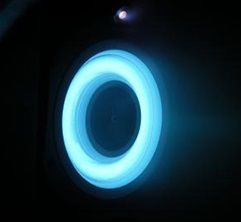
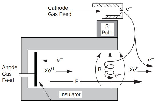
12 Chapter 1. Introduction
(a) Emission from Hall
Effect thruster (b) Operating principle of Hall effect thrusters[]
Figure 1.1: Hall effect Thruster
1.1 Hall effect thrusters
Hall effect thrusters or HET are a special type of electromagnetic thrusters.
They operate at low density with a strong external magnetic field. Figure 1.1
shows a schematic of a typical Hall effect thruster. Electrons emitted from the
cathode enter the channel and are subjected to a radial magnetic field and an
axial electric field. The magnetic field is chosen such as the plasma electrons
are trapped in a E × B drift, usually termed as the Hall current, while ions
are free to accelerate downstream along the electric field between the anode
and the cathode. Hence, electrons acquire a rotational motion around the inner
coil, resulting in an increase in the ion density via electron-impact ionization
ergo an increase in the thrust density.
A serious interest worldwide in this propulsion scheme arose in the 1990s
and more studies were carried out to increase the efficiency of the device. This
is how the study of HET became an important area of plasmas sources re-
search. In recent years, researchers focused on developing simulation codes,
such as Particle-in-cell (PIC) and fluid codes, as well as experimental diagnos-
tic tools, especially optical emission spectroscopy (OES), to extract plasma
parameters. At the Laboratoire de Physique des Plasmas for instance, a huge
emphasis was put on PIC and fluid simulations and the lab owns its own bench-
marked PIC code for HETs. This code simulates multiple plasma parameters
that are usually very difficult to measure experimentally and returns an exten-
sive description of the plasma in the thruster. Today, the lab is looking into
OES to probe the plasma in the HET channel and is investigating ways to cou-
ple the PIC code to experimental input. A promising tool for this purpose is a
collisional radiative model that is presented briefly in the following section.1.2. Collisional radiative models: General introduction 3
1.2 Collisional radiative models: General in-
troduction
Collisional radiative models or C-R models are 0-dimensional models that are
very useful as being complementary to experimental observations. They en-
able relating an observed experimental spectrum, from the plume of a HET
for instance to a simulated spectrum whose electron density and electron tem-
perature are known (see Figure 1.2) hence giving the plasma parameters of
the studied plasma discharge. Such results can be used then in plasma trans-
port models, for example, LPP’s PIC, to obtain simulations close to the real
discharge regime.
The development of C-R models for electric propulsion is relatively recent.
In the literature different models [4, 5, 1, 6] have been developed for different
HET designs and different propellants types. Nevertheless, the following re-
port focuses on the C-R model by Karabadzhak, Chiu, and Dressler [1]. This
research group built a C-R model for xenon that predicts the line intensities for
near-infrared transitions and proposed line ratio curves to estimate the electron
temperature.
Figure 1.2: How to link OES and C-R model results
Here, we present the C-R model developed at LPP. We discuss both the
theoretical and numerical considerations investigated to ensure the stability
and reliability of the model. A C-R model for xenon is then presented in-
volving 15 energy levels. We identify the population density distribution at
steady-state and the dominant kinetics between the levels. After discussing
the impact of other plasma parameters on the population density, we study
the line ratio method developed by Karabadzhak, Chiu, and Dressler [1] and
validate it using our model.Chapter 2
Background
In order to obtain a simulated spectrum using a C-R model, the density of
atomic state levels for all plasma species is calculated using the particle bal-
ance equation. Usually, this equation balances the time-variation of the density
to the density changes due to the convective diffusive transport and the colli-
sional radiative processes. However, for most low temperature plasmas and
in particular those encountered in HETs, the convective diffusive contribution
is negligible in comparison to the collisional radiative contribution [7, 8] and
therefore we can assume ∇(np U) = 0, hence yielding:
∂np ∂np
= (2.1)
∂t ∂t coll,rad
where np is the density of the level p and U is the velocity field vector. The
state density ηp is then related to the level density np through η = ngpp where gp
is the statistical weight of the level p.
Eq.2.1 sets the theoretical background for C-R models. The next step is
to characterize the second term in the equation accounting for the collisional
radiative terms. This is done in the following section.
2.1 Characterising the collisional-radiative pro-
cesses
This section investigates electron-impact excitation and radiative processes
only and develops the theoretical background behind their use in our C-R
model. An exhaustive description of all possible processes can be found, how-
ever, in [9] and is out of the scope of this work.
42.1. Characterising the collisional-radiative processes 5
2.1.1 Electron-impact excitation and de-excitation
Electron-impact excitation
A collision between an atom and an electron may cause the atom to change
its quantum state. In this process, a particle in the excited state gains a certain
amount of kinetic energy equal to the difference in energy between the two
states:
Xp + e− → Xq + e− , where Ep < Eq
where Xk represents an excited atom in the level k.
The probability of such an event happening is determined by the excitation
cross-section from p to q denoted hereafter σpq . This cross-section quantifies
the likelihood of a collision at a specific electron kinetic energy E. The net
transition probability Kpq is then obtained by averaging this cross-section over
the electron energy distribution function (EEDF), thus taking into account all
the different energies. This yields the following expression:
Z ∞ √
r
2
Kpq = σpq E fˆE (E)dE (2.2)
m0 Ep −Eq
R∞
where fˆE is the normalised electron energy distribution such as 0 fˆE (E) =
1. The change rate dndt
p
in Eq.2.1 due to electron excitation is given hence by
ne Np Kpq .
Electron impact de-excitation
In this process, a particle in the excited state loses a certain amount of kinetic
energy by electron impact. The principle of detailed balance provides a simple
expression as Eq.2.2 for the de- excitation process. This principle states that
at equilibrium, each elementary process is balanced by its reverse process[10,
11, 12], resulting in the equality of rates:
ne np Kpq = ne nq Kqp
where np and nq are the level density corresponding to the excited levels p
and q. Assuming a thermodynamic equilibrium for instance, the Maxwell-
Boltzmann distribution applies yielding:
np nq Ep − Eq
= exp(− ) (2.3)
gp gq kb Te6 Chapter 2. Background
where kb is the Boltzmann constant and Te is the electron temperature. We
can now relate the rate coefficient for electron-impact excitation Kpq to that of
electron-impact de-excitation Kqp by the following expression:
gp Epq
Kqp = Kpq exp(− ) (2.4)
gq kb Te
Hence, the change rate dndt
p
in Eq.2.1 due to electron de-excitation is given by
ne Nq Kqp . In case the Maxwellian EEDF does not apply, a similar formula can
be obtained and the derivation is reported to Appendix A. This case was imple-
mented in the code but is not used in this report since we assumed Maxwellian
EEDF.
2.1.2 Emission and absorption
The approach to modeling emission and absorption is reported to Appendix.B.
This section sums up briefly the main theoretical aspects.
The biggest difficulty in treating radiative processes is juggling the local
nature of spontaneous emission and the non-local nature of absorption and
stimulated emission. Holstein [13] and Irons [14] circumvent this problem by
introducing a dimensionless parameter Γpq , termed "Escape Factor" that arti-
ficially expresses the amount of radiation absorbed as a percentage of the total
spontaneous radiation emitted. Put differently, this parameter conveniently
reduces the non-local effect of absorption to a mere percentage of the sponta-
neous emission along the line of sight. Ergo, the net change term due to radi-
ation in Eq.2.1, i.e the change term from emitted radiation minus the change
term from absorbed radiation, can be expressed simply as:
Γpq Apq np
where Aqp is the corresponding Einstein coefficient for the transition from level
p to level q. The escape factor depends on the geometry of the medium, the
nature of the transition and the line frequency profile via the optical depth.
And in the case of a uniform cylindrical plasma column, which is a good first
approximation for HET plasmas, it can be expressed as follows:
c2 gp
τν = Apq P0 nd R (2.5)
8πν 2 gq
where gp and gq are the statistical weights for the upper and lower level of
the transition, respectively, nd is the density of the lower level along the line2.2. Karabadzhak C-R model 7
of sight and P0 is the value at the center of the line frequency profile. P0 is
calculated theoretically based on a Voigt profile that accounts for both natural
and Doppler broadening (cf. Appendix B). Then, using Mewe [15] empirical
formula, the escape factor can be calculated as follows:
2 − exp(−τν /1000)
Γpq = (2.6)
1 + τν
where τν is the optical depth of the medium for the specific frequency ν. This
expression is usually valid for most low temperature plasma as discussed by
Bhatia and Kastner [16] and Irons [14] in their respective articles.
2.1.3 Balance equation of the collision radiative model
If we incorporate the processes discussed before in 2.1, the time-dependent
differential equation for a given level p can be written as follows:
dnp X X X
= Kqp ne nq − Kpq ne np + Γqp Aqp nq − Γpq Apq np (2.7)
dt q p8 Chapter 2. Background
coupled to the ground state via a resonant level. The electron excitation cross-
section from metastables was not calculated and was assumed to be propor-
tional to the statistical weight of the 2p levels.
The use of the emission cross-section makes the Karabadzhak approach
"line-oriented" expressing analytically the intensity of each line in function of
the processes contributing exclusively to the intensity of the line. According
to [1], the intensity of a line at the wavelength λ is expressed as follows:
hc Nm λ 1−α λ
Iλ (Xe) = N0 Ne (keλ0 + kem + αk1λ + k2 ) (2.8)
4πλ N0 2
where keλ0 and kemλ
are the rate coeficients for excitation from the ground state
λ
to an excited level to produce the radiation λ, kem is the rate coeficient for
excitation from the metastables, ie 1s5 and 1s3 to the same excited level to
produce the radiation λ, k1λ and k2λ are the emission excitation rate coefficients
for collisions of Xe+ and Xe2+ with neutral xenon atoms, Nm is the density of
the metastables and N0 is the ground state density, α is the ratio of Xe+ to the
electron number density.
Table 2.1: Levels involved in the expression of the line intensity of the transi-
tion in the model of Karabadzhak
Transition Wavelength [nm] Levels involved
2p6 → 1s5 823 gs 2p6 1s5 1s4
2p6 → 1s5 828 gs 2p5 1s4
2p6 → 1s5 834 gs 1s2 2p3
Additional experimental work identified three relevant transitions for op-
tical diagnostics. These are reported to Table 2.1. Using the C-R model and
Eq.2.8, the intensity ratio of the 823-828 nm and the 834-828 nm were calcu-
lated for different electron temperature input. And the results are presented in
Figure 2.1
These curves are very useful for optical diagnostic since it allows to extract
the electron temperature from simple ratio calculations. For this reason, we
would like to reproduce these curves using our home-made C-R model. The
method for this purpose is exposed in the following chapter.2.2. Karabadzhak C-R model 9
1.0 10
Kar Kar
0.8 8
0.6 6
I834/I828
I823/I828
0.4 4
0.2 2
0.0 0
0.0 2.5 5.0 7.5 10.0 12.5 15.0 17.5 20.0 2.5 5.0 7.5 10.0 12.5 15.0 17.5 20.0
Te (eV) Te (eV)
Figure 2.1: Calculated electron temperature dependence on the intensity ratios
of the Xe lines 823/828nm and 834/828nm[1]Chapter 3
Methods
3.1 LPP0D Xenon C-R model
The C-R model developed at LPP is called LPP0D and is dedicated to xenon.
The code aims to solve Eq.2.7. With that end in view, we defined first the
species present in the system, the levels considered in the balance equation
and the processes involved. Second, we gathered appropriate cross-section
data and radiative data with an eye to calculate the rate coefficient and the
escape factor. Third, we chose appropriate numerical methods well-suited for
our type of data. And finally, we ran some tests to validate the code. In the
following section, the reader can find more details about our approach.
3.1.1 Processes and levels
Only neutral Xe was considered in LPP0D. Processes involving Xe+ and Xe2+
were not included. The model is limited to the Xe(5p5 5s) and Xe(5p5 6p) con-
figurations, who correspond to the 1s and 2p manifolds in Paschen’s notations
(refer to [11]). The data is retrieved from NIST database [18]. of the Ap-
pendix. We only considered these levels because we believe they are the most
important levels when it comes to optical emission which is also confirmed by
the work of Karabadzhak, Chiu, and Dressler [1].
As for the processes considered in LPP0D, we considered all the electron-
impact excitation and de-excitation between the excited levels, as well as the
spontaneous emission and absorption using the escape factor approximation.
103.1. LPP0D Xenon C-R model 11
[32]o2 [32]o1 [12]o0 [12]o1 [12]1 [52]2 [52]3 [32]1 [32]2 [12]0 [32]1 [32]2 [12]1 [12]0 [12]o0 [12]o1 [72]o4 [72]o3 [32]o2 [32]o1 [52]o2 [52]o3 [52]o2 [52]o3 [32]o2 [32]o1
s5 s4 s3 s2 p10 p9 p8 p7 p6 p5 p4 p3 p2 p1 d6 d5 d 4' d4 d3 d2 d 1" d1' s1"" s1"' s1" s 1'
J= 2 1 0 1 1 2 3 1 2 0 1 2 1 0 0 1 4 3 2 1 2 3 2 3 2 1
2
P1/2 ion core
13
7s' 2
P3/2 ion core
12 5d'
7p 6p' 6d
11 7s
Energy (eV)
5d
6p
10 6s' 5
5 5p 5d
5p 6p
9
6s 5p56s
8
1
0 1
S0
2
1s ...5p
6 Xe
©2002 Atom Weasels
Figure 3.1: Diagram showing the excited levels of Xe included the model: in
red the 1s multiplet and in green the 2p multiplet
3.1.2 External data
Cross section
Since xenon is not a commonly used element in the low-temperature plasma
community, there have not been extensive measurement campaigns to cover all
the electron-impact excitation included in LPP0D. For this reason, we relied on
numerical methods. These methods have been proven to be in good agreement
with experiments as discussed in Bordage et al. [19] review. Two methods are
used in LPP0D to build a complete data set for xenon which are the Distorted-
Wave approach [4] and the semi-relativistic B-spline R-matrix (BSR) method
[20]. Table 3.1 shows in details the references for every excitation processes.
EEDF
Maxwellian EEDF was used for this report. Usually, this assumption is suf-
ficient to describe the plume region in Hall effect thruster [6] and to draw
some conclusions about the kinetics of the excited levels and optical diagnos-
tics. Nevertheless, the code, however, was implemented with an eye to support
other types of EEDF, such as Burgrova distributions [6] and sampled PIC dis-12 Chapter 3. Methods
Table 3.1: The collisional processes included in our model. The third column
gives the refrences for the cross sections
Excitation Process Reference
From the ground state Xe(gs) + e−1 → Xe∗ + e−1 [20, 21]
1s Mixing Xe∗ (1s) + e−1 → Xe∗ (1s) + e−1 [4]
2p Mixing Xe∗ (2p) + e−1 → Xe∗ (2p) + e−1 [4]
From 1s to 2p Xe∗ (1s) + e−1 → Xe∗ (2p) + e−1 [4, 22]
tributions.
Radiative data
Einstein coefficients were retrieved from NIST database [18]. Mewe approxi-
mation (Eq.2.6) was used for the escape factor and Eq.2.5 was used to calculate
the optical depth. The value of the line profile at the center was estimated with
a Voigt profile (cf. Appendix B)
3.2 The Code
3.2.1 Numerical methods
Data and Sampling
LPP0D relies primarily on sampled data, either for cross-section data or for
EEDF distributions. At different levels of the code, this data is interpolated
or integrated, and if the quality of the sample is not ensured, these operations
might introduce additional numerical bias. A big effort during this project
was to conservatively estimate this bias. Different interpolation and integra-
tion schemes were investigated using both theoretical and real cross-sections.
Going through all the tests performed is out of the scope of this report and we
only present the main conclusions and measures implemented in the code.
We ensured that all cross-section data set for LPP0D were defined on a win-
dow of 300 eV at least. The sampling pace was defined by the reference article
so we could not control it. However, the sample was enriched using linear in-
terpolation to ensure a sampling pace of 0.03 eV near the energy threshold and
0.3 eV far from the threshold. A simple linear scheme was enough since us-
ing a higher level interpolation scheme involved more work while not yielding
significant improvement on the numerical results.3.3. Test cases 13
Maxwellian EEDFs were also defined on a window of 300 eV and with
a sampling pace of 0.03 eV. All this ensured a conservative precision of the
collisional terms of at least 11% for a temperature range of 0-40 eV.
The integration method used for calculating the value at the center of the
line profile (Eq.B.3) was a Gauss-quadrature method. The precision of the
returned value was up to 5 digits and was verified using MATLAB and Math-
ematica.
ODE solver
The processes included in Eq.2.1 occur at different time scales of different
magnitude. Typical time scale for radiative transitions is 10−5 − 10−8 s, while
for collisional excitation, it is around 10−3 − 10−1 s. This might lead to certain
levels evolving faster then others making classical integration methods such
as Euler or Newton, completely inefficient.
Backward Differentiation Formula (BDF) scheme [23] is perfectly fit for
these situations and was the main solver for LPP0D. The implementation of the
solver, the stability and accuracy of the solver are discussed in the following
paper by Byrne and Hindmarsh [24]. Using complementary information from
[25, 26, 27], we verified in a conservative manner that our initial conditions
fall into the stability region.
3.2.2 Structure overview
A builder module named objects_generator parses the list of the selected re-
actions and fetches the needed data sets to calculate the electronic collisions
rate coefficients and the radiative emission data. A different builder mod-
ule, diff_generator, creates the corresponding set of the differential equations.
These are then sent to the BDF solver to retrieve an array of the level densi-
ties time-evolution. Then to retrieve the state density η, the result is divided
by the statistical weights. Additional methods for spectrum generation and
source/loss terms analysis were implemented along with the core code.
3.3 Test cases
3.3.1 2 levels collisions
Here, only two xenon levels were considered, for example Xe(gs) and Xe(1s4).
Electronic excitation and de-excitation were the only processes involved. In14 Chapter 3. Methods
Figure 3.2: Computed and analytical time evolution of the density of the two
state levels. Parameters: Xenon, ne =1 × 10¹⁷ m−3 , ng =1 × 10⁻²⁰ m−3 , Tg =
300 K, Maxwellian EEDF at 15 eV
this case, the Eq.2.1 was solved analytically and the density of each level was
given by:
(
nXegs (t) = n0 − n1s2 (t)
Kgs→1s2 (3.1)
nXe1s4 = n0 (1 − Kgs→1s2 +K1s2→gs
)(1 − e−(Kgs→1s2 +K1s2→gs )ne t )
From 3.1, the output of the model were compared to the analytical expression
in Figure 3.2. It showed a very good agreement and verified the aforemen-
tioned stability of the integration scheme.
3.3.2 Steady state for 3 levels with radiative cascade
We considered then three levels that involved a radiative cascade. For exemple
Xe(gs), Xe(1s4) and Xe(2p1). Only electron-impact from the ground state to
2p1 was considered. The Xe(2p6) de-excites radiatively to Xe(1s4) that de-
excites also radiatively to the ground states. Assuming steady state in Eq.3.1,
we expressed the final densities as follows:
n
Xegs 1
ne
= Kgs→2p1 K
+ A gs→1s2
1+
A2p1→1s4 1s4→gs
nXe 1
1s4
ne
= A A (3.2)
1+ A 1s4→gs + K1s4→gs
2p1→1s4 gs→2p1
nXe2p1
= A2p1→1s41 A2p1→1s4
ne
1+ +
Kgs→2p1 Kgs→2p13.3. Test cases 15
where Kgs→2p1 is the rate coefficient for the electron-impact excitation from
the ground state to 2p1, and A2p1→1s4 and A2p1→1s4 are the Einstein coeffi-
cients for the Xe(2p6) to Xe(1s4) transition and the Xe(1s4) to ground state
transition, respectively. We ran the code for different electron temperatures
and compared the output at the steady-state with the analytical results. We
verified that it gave a good agreement.
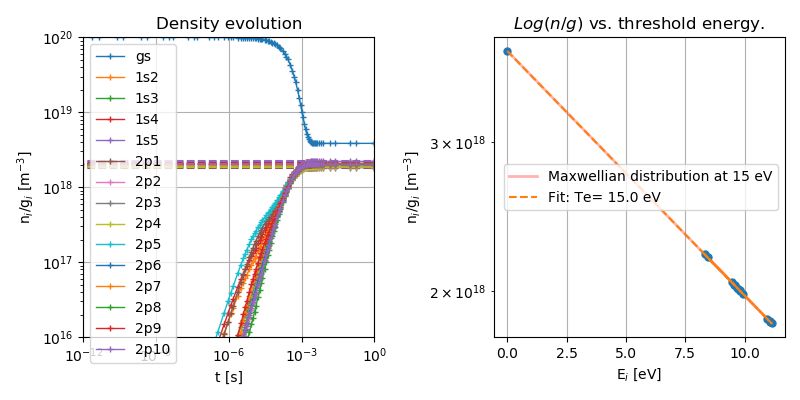
3.3.3 Thermal equilibrium
Figure 3.3: Time evolution of the population density and the Boltzmann
plot under the assumption of a thermal equilibrium. Parameters: Xenon,
ne =1 × 10¹⁷ m−3 , ng =1 × 10⁻²⁰ m−3 , Tg = 300 K, Maxwellian EEDF at
15 eV
Finally, we looked into the case of thermodynamic equilibrium. We se-
lected all xenon levels used in the model ie ground state, 1s, and 2p levels.
Electron-impact excitation was balanced with its corresponding inverse reac-
tions, thus ensuring micro-reversibility. The emitted radiation is equal to the
absorbed radiation, thus ensuring a null net radiative bracket, Γ = 0 (Black
body radiation). We additionally assumed a Maxwellian EEDF. At steady state
the system reaches thermodynamic equilibrium and the levels densities follow
a Boltzmann distribution such as:
ni gi Ei
= e Te
n0 Z
where Z is the partition function of the system, gi is the statistical weight of
level i, Ei is the energy of the level i and Te is the electron temperature.16 Chapter 3. Methods
Figure 3.3 shows the temporal evolution obtained from the C-R model as
well as the density of each level in the function of its energy. As expected from
theory, the levels are aligned along a straight line whose slope is equal to T1e
on a logarithmic scale. The linear regression yields a very good correlation
factor of r2 = 1
3.4 Karabadzhack method
To obtain the line ratio curves using LPP0D, we verified the validity of the
assumptions made in [1] by investigating the dominant kinetic processes be-
tween the excited levels. This is discussed in section 4.1. Once the assump-
tions were verified, we designed three input models to study each transition
line separately in conformity with Karabadzhack’s approach. Figure 3.4 and
Table 2.1 give the levels and processes for each transition. Ionization was not
taken into account because it is not currently supported by the code. For the
2p3 2p5
834nm 828nm
e- impact e- impact
1s3 1s4
129nm 145nm
gs gs
(a) The 834 nm transition (b) The 828 nm transition
2p6
895.2nm 823.2nm
e- impact
1s4 1s5
145nm
gs
(c) The 823 nm transition
Figure 3.4: Diagram of the processes and levels involved in the transitions
selected by Karabadzhack for OES diagnostics
823 nm transition, the rate coefficient from 1s5 was defined with a proportion-
ality factor in the article. This factor was estimated empirically to 10−12 using
LPP0D so that to ensure the best fit.Chapter 4
Results
We present first a brief study of the kinematics of the excited levels and explicit
the dominant processes between the 1s and the 2p multiplets. We present then
the results of several parametric studies highlighting the impact of the gas
density, the electron temperature, the electronic density and the EEDF on the
overall population density. We finally compare the LPP0D results for the line
ratio for the 823-828 and 834-828 lines with the curves from [1].
4.1 Parametric study on pure xenon
4.1.1 Density population
Figure 4.1 shows the evolution and steady-state of the xenon discharge in the
HET when the black body equilibrium is no longer verified. It can be seen that
the distribution no longer follows a Boltzmann distribution. The population of
the radiatively linked levels, 2p levels mainly, is the most impacted and their
respective state density is lower. This highlights that for these levels, radiative
processes are more dominant than electron-impact excitation.
On the pure emission case, the 1s multiplet can be divided into two groups.
The first one includes the metastable states 1s5 and 1s3 while the other con-
tains the resonant levels 1s2 and 1s4. Similarly to the 2p levels, the resonant
levels are radiatively linked to the ground state so that their population is low.
The metastables de-populated through collisions only and have higher densi-
ties
Adding absorption to the equation using Mewe approximation, the impact
of emission is reduced and this allows electron-collisions to have more impact
on levels with close energies. The population of excited levels increased due
1718 Chapter 4. Results
Pure emission = 1 Mewe approximation 0
1020 1020
1019 1019
1018 1018
ni/gi [m 3]
ni/gi [m 3]
1017 1017
1016 1016
1015 1015
0 2 4 6 8 10 0 2 4 6 8 10
Ei [eV] Ei [eV]
gs 1s3 1s5 2p2 2p4 2p6 2p8 2p10
1s2 1s4 2p1 2p3 2p5 2p7 2p9
Figure 4.1: Impact of the absorption using the escape factor approximation
on the density population. In red, the 15 eV line representing a Maxwellian
distribution. Parameters: Xenon, ne =1 × 10¹⁷ m−3 , ng =1 × 10²⁰ m−3 , Tg =
300 K, Maxwellian EEDF at 15 eV
to radiation trapping. Figure 4.1 highlights 4 groups that have an equilibrium-
like distribution: 1s5 − 1s4, 1s3 − 1s2, 2p10 − 2p5 and 2p4 − 2p1. Also, these
levels are not affected homogeneously by the radiative processes. For instance,
the strong radiative lines 2p5-2p10 are strongly de-populated by spontaneous
emission compared to the 2p1-2p4 levels.
4.1.2 Dominant kinetic processes
For each level, we quantified the contribution of the different processes to the
population or de-population of the level. Given a process A, the loss or the
creation contribution was defined as the ratio of the change rate corresponding
to A, divided by the total change rate corresponding to the population of the
level or the depopulation of the level respectively. An example of the results
can be seen in Figure 4.2. Figure 4.3 sums the results from all the 15 levels
in a single diagram that maps the important processes for each of the groups
identified previously.
The kinetics between the ground state and 1s or 2p is dominated by elec-
tron -impact excitation. The 2p multiplet is populated by collisions from the
ground state and de-populates radiatively to the 1s. The kinetics between the
2p multiplet and the 1s depends on the subgroup. The first one including 2p1
to 2p4 levels. They have large excitation rate coefficients from 1s3 and 1s24.1. Parametric study on pure xenon 19
Creation Loss
InvExc gs 2p10 Exc gs 1s3
InvExc gs 1s5 Exc gs 2p10
InvExc gs 2p9 Exc gs 2p6
InvExc gs 1s3 Exc gs 2p8
InvExc gs 1s2 Exc gs 1s5
InvExc gs 2p1 Exc gs 2p9
InvExc gs 1s4 Exc gs 2p1
InvExc gs 2p5 Exc gs 2p5
Rad 1s2 gs Exc gs 1s2
Rad 1s4 gs Exc gs 1s4
10 4 10 2 100 10 4 10 2 100
Process contribution for Xe(gs)
Figure 4.2: Histogram of the contribution of creation and loss terms for the
ground state. Parameters: Xenon, ne =1 × 10¹⁷ m−3 , ng =1 × 10²⁰ m−3 , Tg =
300 K, Maxwellian EEDF at 15 eV
gs
exc exc
1s4-1s5 1s3-1s2
exc exc
rad rad
2p5-2p10 2p1-2p4
Figure 4.3: Dominant kinetic processes between the 1s and 2p multiplet. In
green: electron-impact excitation. In yellow: radiative transitions. Parame-
ters: Xenon, ne =1 × 10¹⁷ m−3 , ng =1 × 10²⁰ m−3 , Tg = 300 K, Maxwellian
EEDF at 15 eV20 Chapter 4. Results
(Appendix.E) and mainly de-populate radiatively to these levels. On the other
hand, the second group from 2p5 to 2p10 have a large excitation rate coefficient
from 1s4 and 1s5 (Appendix.E).
4.1.3 Gas density
The gas density intervenes in the model at two different places. The gas density
can affect the electron-impact collisions from the ground states and radiation
trapping.
Pure emission = 1 Mewe approximation 0
1022 1022
1020 1020
ni/gi [m 3]
ni/gi [m 3]
1018 1018
1016 1016
1014 1014
0 2 4 6 8 10 0 2 4 6 8 10
Ei [eV] Ei [eV]
ng = 1e + 19 ng = 1e + 20 ng = 1e + 21 ng = 1e + 22
Figure 4.4: Impact of the gas density on the density distribution. The dashed
line are linear fits highlighting how close is the distribution to thermal equilib-
rium. Parameters: Xenon, ne =1 × 10¹⁷ m−3 , Tg = 300 K, Maxwellian EEDF
at 15 eV
Figure 4.4 shows the impact of the gas density at a constant temperature
Tg = 300 K on the steady-state distribution. In the pure emission case, the
distribution is simply shifted vertically with no change in the ratios between
the state densities. This suggests that ng should be treated as a scaling factor
for future simulations. If absorption is taken into account, we can observe a
similar behavior along with a change of the slope. The higher the gas density
is, the more opaque the system becomes and more radiation is absorbed hence
increasing the overall population of the excited levels.4.1. Parametric study on pure xenon 21
Pure emission = 1 Mewe approximation 0
1022 1022
1020 1020
ni/gi [m 3]
ni/gi [m 3]
1018 1018
1016 1016
1014 1014
0 2 4 6 8 10 0 2 4 6 8 10
Ei [eV] Ei [eV]
Te = 5eV Te = 15eV Te = 20eV Te = 25eV
Figure 4.5: Impact of the electron temperature on the density distribution.
Parameters: Xenon, ne =1 × 10¹⁷ m−3 , ng =1 × 10²⁰ m−3 , Tg = 300 K.
4.1.4 Electron temperature and electronic density
The electron temperature affects the shape of the EEDF and for a Maxwellian
EEDF, it is related to the mean energy via E = 23 kB Te . At high electron tem-
perature, more energetic particles will contribute to collisions in the plasma
thus increasing collision probability, i.e the rate coefficient. Figure 4.5 shows
the impact of Te on the shape of the Boltzmann plot.
The slope of the linear regression decreases suggesting an increase in the
population of the excited levels. However, this variation is barely visible for
Te > 15 eV. The population density distribution varies little beyond that limit
suggesting that OES methods are extremely sensitive if the Te < 15 eV. This
can be seen on Karabadzhak line ratio curves (Figure 3.4) where the ratio
reaches a plateau very quickly at around 15 eV. A similar behavior can be
seen also while changing the electronic density, as shown in Figure 4.6.22 Chapter 4. Results
Pure emission = 1 Mewe approximation 0
1022 1022
1020 1020
ni/gi [m 3]
ni/gi [m 3]
1018 1018
1016 1016
1014 1014
0 2 4 6 8 10 0 2 4 6 8 10
Ei [eV] Ei [eV]
ne = 1e + 17 ne = 1e + 18 ne = 1e + 19 ne = 1e + 20
Figure 4.6: Impact of the electron density on the density distribution. Param-
eters: Xenon, Tg = 300 K, Maxwellian EEDF at 15 eV
4.1.5 Net radiative bracket
The net radiative bracket depends on three major parameters: the geometrical
scaling factor R, the density population of the lower level and finally the mag-
nitude of the broadening of the line. All these parameters act via the optical
depth parameter τ (See Eq.2.5).
Escape factor as function of the optical depth
1.0
0.8
0.6
0.4
0.2
0.0
10 3 10 1 101 103
Optical depth [m 1]
Figure 4.7: Numerical escape factor as a function of the optical depth
Figure 4.7 shows the dependency of the escape factor on τ while Figure 4.8
shows the temporal evolution of the escape factor in function of the transition
line. The medium is transparent in the beginning (Γ = 1). As soon as the pop-
ulation of the excited levels increases, τ increases and the medium becomes
more opaque to radiation. Most of the lines, at steady state, have a black-body
like net radiative bracket (Γ ≈ 0). This is coherent with the previous remarks4.2. Line ratios 23
about how the state density distribution is closer to a Boltzmann-like equilib-
rium when the absorption is included. 2p1, 2p3 and 2p4 are the only levels to
have a high escape factor.
1
1s2->gs 1s4->gs
0
10 16 10 14 10 12 10 10 10 8 10 6 10 4 10 2 100
1
2p1->1s2 2p3->1s2
2p2->1s2 2p4->1s2
0
10 16 10 14 10 12 10 10 10 8 10 6 10 4 10 2 100
1
2p2->1s3 2p4->1s3
0
10 16 10 14 10 12 10 10 10 8 10 6 10 4 10 2 100
1 2p1->1s4 2p6->1s4
2p3->1s4 2p7->1s4
2p4->1s4 2p9->1s4
2p5->1s4 2p10->1s4
0
10 16 10 14 10 12 10 10 10 8 10 6 10 4 10 2 100
1 2p2->1s5 2p7->1s5
2p3->1s5 2p8->1s5
2p4->1s5 2p9->1s5
2p6->1s5 2p10->1s5
0
10 16 10 14 10 12 10 10 10 8 10 6 10 4 10 2 100
Figure 4.8: Time evolution of the escape factor for different transitions.
Parameters: Xenon, ne =1 × 10¹⁷ m−3 , ng =1 × 10²⁰ m−3 , Tg = 300 K,
Maxwellian EEDF at 15 eV, Plasma column radius 10cm
4.2 Line ratios
The study of the dominant kinetics showed that the assumptions of Karabadzhak
et al. are valid. The 2p multiplet populates through electron-impact excitation24 Chapter 4. Results
1.0 10
ne = 7e + 17 ng = 1e + 20 ne = 7e + 17 ng = 1e + 20
Kar Kar
0.8 8
0.6 6
I834/I828
I823/I828
0.4 4
0.2 2
0.0 0
0.0 2.5 5.0 7.5 10.0 12.5 15.0 17.5 20.0 0.0 2.5 5.0 7.5 10.0 12.5 15.0 17.5 20.0
Te (eV) Te (eV)
Figure 4.9: Calculated electron temperature dependency on the line intensity
ratios of 823-828 and 834-828 using LPP0D
and de-populates radiatively via a radiative cascade. The line ratio curves for
823-828 nm and the 834-828 nm ratios were calculated individually in sep-
arate models for a gas density ng = 1020 m−3 and a typical electron density
ne = 1017 m−3 . Figure 4.9 shows a relatively good agreement for the 823-828
nm ratio and a less good agreement for the 834-828 nm ratio.Chapter 5
Discussion and open questions
5.1 Assumptions in the C-R model
The first important assumption in our C-R model is how many energy levels
should we take to have an accurate description of the kinetics. In our model,
we limited the model to 1s and 2p multiplets, usually done in the literature.
Figure 3.1 highlights however that 7s and 7p levels are close energy-wise to
the 2p multiplets and are likely to interact radiatively or via collisions. The
contributions of these levels were not studied in this work and is a task for
future investigations. A recent C-R model by Zhu et al. [6] included these
levels and did not show very different kinetics for the 2p as it is described
here.
The second important assumption is the nature of the processes taken in
our model. It was limited to electron-impact excitation and radiative emis-
sion/absorption. Other processes could have been included like atom-atom
collisions, electron-impact ionization, diffusion, etc ... However, at a low tem-
perature, many of these processes are negligible which was verified a priori.
Karabadzhak, Chiu, and Dressler [1] highlight in their article the importance
of ion-atom collisions. They include to that purpose Xe+ and Xe2+ in their
model. This might explain the less good agreement for the 834-828 nm ra-
tio. Nevertheless, we could not do better since excitation cross sections for
the fine-structure of Xe+ and Xe2+ are unavailable in the literature limiting
temporarily the scope of our model. But it will be included in future works.
The third important assumption is the escape factor. We opted in our
model for Mewe’s empirical formula. This formula delivers usually satisfac-
tory agreement with experiments, and that is what makes its popularity among
plasma modelers. Recent work by Zhu et al. [28] improved this formula for
2526 Chapter 5. Discussion and open questions
xenon and tailored an escape factor formula for each radiative transition. The
improvement brought to the model from the use of these level-specific escape
factor is yet to be quantified and will be the subject of future work.
The fourth important assumption is the calculation of the rate coefficient.
Many C-R models use either theoretical cross-sections based on the Bethe-
Born approximation or empirical formulas that involve the oscillator strength
[9]. These formulas are usually accurate at very high energies but do not de-
liver accurate results at low energies, typically 0.1 eV for 2p collisions for
instance. That’s why the usage of measured/calculated cross-sections seems
very reasonable in our case even if it introduces a numerical bias that we con-
servatively quantified (cf. Section 3.2.1).
Finally, the fifth important assumption is Maxwellian EEDF. As mentioned
in the introduction the main purpose of this project is to use the C-R model on
an EEDF from a PIC simulation. However, we only investigated Maxwellian
EEDF that is primarily found in the plume of the HET. Different parts of the
thruster could be investigated with other theoretical distributions such as Bu-
grova distribution for the discharge channel [6] and are considered for future
developments of the code. Meanwhile, a new set-up is being designed to per-
form OES inside the HET and to use the C-R model for comparison.
5.2 Numerical biais
A conservative estimation of the numerical bias on the results from LPP0D
was estimated to 11% as mentioned in 3.2.1. We opted for a linear numer-
ical interpolation scheme and a BDF integration method. Several classical
interpolations and integration methods were investigated with theoretical and
real cases. However, the gain in accuracy was uninteresting compared to the
computational cost. The most proper approach to improve the accuracy of the
sampled data is to use a Gaussian process regression [29] instead of simple
interpolation. The idea is to perform several Monte-Carlo simulations based
on a predefined Gaussian model and then vary the parameter of the model
until a satisfactory trust interval is reached. This might be used for further
improvement of the code5.3. Karabadzhak near-infrared C-R model for xenon 27
5.3 Karabadzhak near-infrared C-R model for
xenon
The agreement between LPP0D and Karabadzhak curves was at the expense
of separating the transitions and reducing the numbers of levels. Since both
models have a different approach to the C-R model, this artifact was neces-
sary. The 823-828 nm ratio gave a good agreement whereas the 834-828 nm
was less satisfying. One possible explanation is ionization since Karbadzhak
highlights in his article [1] that electron-impact ionization is critically impor-
tant at low temperatures. That’s why for future work we will try to include this
process into LPP0D.Chapter 6
Conclusion
HETs have become today a very important plasma source in plasma physics
research. Most of the investigation carried out in the literature rely historically
on experimental measurement and today a new interest in numerical simula-
tions has arisen, motivated mainly by reducing the test costs. The ambition
of this work is to provide a C-R model that bridges between PIC simulation
results and OES measurements. To this purpose, we studied the theoretical
background for the C-R model and tried to build a comprehensive theory start-
ing from fundamental physics, especially for radiative processes. We explored
then different numerical aspects of the code:
• First, quantify the systematic error linked to sampling
• Second, try different numerical integration and interpolation schemes to
decide the best
The validity of the model was assessed using the thermal equilibrium hypoth-
esis.
Running the model under HET conditions allows mapping the dominant
kinetics between the excited levels. The 2p multiplet populates mainly radia-
tively and consists of two subgroups: The first de-excites to 1s3 − 1s2 and the
second de-excites to 1s4 − 1s5. This enables to simplify the model since fine-
structure excitations are negligible, hence supporting the Karabadhzac model.
A further comparison with Karabadhzac’s work yields a good agreement on
the overall behavior of the line ratios. Nevertheless, it needs more improve-
ment mainly by including atom ions interaction in the model
28Bibliography
[1] George F. Karabadzhak, Yu-hui Chiu, and Rainer A. Dressler. “Pas-
sive optical diagnostic of Xe propelled Hall thrusters. II. Collisional-
radiative model”. In: Journal of Applied Physics 99.11 (June 2006),
p. 113305. issn: 0021-8979. doi: 10 . 1063 / 1 . 2195019. url:
https://aip.scitation.org/doi/10.1063/1.2195019.
[2] Edgar Y. Choueiri. “New Dawn for Electric Rockets”. en. In: Scien-
tific American 300.2 (2009), pp. 58–65. issn: 0036-8733. doi: 10 .
1038/scientificamerican0209-58. url: https://www.
nature.com/scientificamerican/journal/v300/n2/
full/scientificamerican0209-58.html (visited on 10/08/2018).
[3] R. G. Jahn. Physics of Electric Propulsion. en. 1968. url: https://
www.ebay.com/itm/Physics-of-Electric-Propulsion-
by-Robert-G-Jahn-English-Paperback-Book-Free-
S-/391203932176 (visited on 10/08/2018).
[4] Priti, R. K. Gangwar, and R. Srivastava. “Collisional-radiative model of
xenon plasma with calculated electron-impact fine-structure excitation
cross-sections”. en. In: Plasma Sources Science and Technology 28.2
(Feb. 2019), p. 025003. issn: 0963-0252. doi: 10 . 1088 / 1361 -
6595/aaf95f. url: https://doi.org/10.1088%2F1361-
6595%2Faaf95f.
[5] Takashi Fujimoto. “Collisional-Radiative Calculation of the Population
Inversion in the Argon Ion Laser”. en. In: Japanese Journal of Applied
Physics 11.10 (Oct. 1972), p. 1501. issn: 1347-4065. doi: 10.1143/
JJAP . 11 . 1501. url: https : / / iopscience . iop . org /
article/10.1143/JJAP.11.1501/meta.
[6] Xi-Ming Zhu et al. “A xenon collisional-radiative model applicable to
electric propulsion devices: II. Kinetics of the 6s, 6p, and 5d states of
atoms and ions in Hall thrusters”. en. In: Plasma Sources Science and
2930 BIBLIOGRAPHY
Technology 28.10 (Oct. 2019), p. 105005. issn: 0963-0252. doi: 10.
1088/1361- 6595/ab30b7. url: https://doi.org/10.
1088%2F1361-6595%2Fab30b7.
[7] David Robert Bates, A. E. Kingston, and R. W. P. McWhirter. “Recom-
bination between electrons and atomic ions, I. Optically thin plasmas”.
In: Proceedings of the Royal Society of London. Series A. Mathematical
and Physical Sciences 267.1330 (May 1962), pp. 297–312. doi: 10.
1098/rspa.1962.0101. url: https://royalsocietypublishing.
org/doi/abs/10.1098/rspa.1962.0101.
[8] J. A. M. van der Mullen. “Excitation equilibria in plasmas; a classifi-
cation”. In: Physics Reports 191 (July 1990), pp. 109–220. issn: 0370-
1573. doi: 10.1016/0370- 1573(90)90152- R. url: http:
//adsabs.harvard.edu/abs/1990PhR...191..109V.
[9] G. J. Tallents. An Introduction to the Atomic and Radiation Physics
of Plasmas. en. Feb. 2018. doi: 10.1017/9781108303538. url:
/core/books/an-introduction-to-the-atomic-and-
radiation-physics-of-plasmas/D9037EF126138DDE37843DB2664230E6.
[10] Detailed balance. en. Page Version ID: 933833660. Jan. 2020. url:
https : / / en . wikipedia . org / w / index . php ? title =
Detailed_balance&oldid=933833660.
[11] Igor I. Sobel’man, Leonid Vainshtein, and Evgenii A. Yukov. Excitation
of Atoms and Broadening of Spectral Lines. en. 2nd ed. Springer Series
on Atomic, Optical, and Plasma Physics. Berlin Heidelberg: Springer-
Verlag, 1995. isbn: 9783540586869. doi: 10.1007/978-3-642-
57825- 0. url: https://www.springer.com/gp/book/
9783540586869.
[12] A. Hartgers et al. “CRModel: A general collisional radiative modeling
code”. en. In: Computer Physics Communications 135.2 (Apr. 2001),
pp. 199–218. issn: 0010-4655. doi: 10.1016/S0010-4655(00)
00231-9. url: http://www.sciencedirect.com/science/
article/pii/S0010465500002319.
[13] T. Holstein. “Imprisonment of Resonance Radiation in Gases”. In: Phys-
ical Review 72.12 (Dec. 1947), pp. 1212–1233. doi: 10.1103/PhysRev.
72.1212. url: https://link.aps.org/doi/10.1103/
PhysRev.72.1212.BIBLIOGRAPHY 31
[14] F. E. Irons. “The escape factor in plasma spectroscopy—I. The escape
factor defined and evaluated”. en. In: Journal of Quantitative Spec-
troscopy and Radiative Transfer 22.1 (July 1979), pp. 1–20. issn: 0022-
4073. doi: 10.1016/0022- 4073(79)90102- X. url: http:
/ / www . sciencedirect . com / science / article / pii /
002240737990102X.
[15] R. Mewe. “Relative intensity of helium spectral lines as a function of
electron temperature and density”. en. In: British Journal of Applied
Physics 18.1 (Jan. 1967), p. 107. issn: 0508-3443. doi: 10 . 1088 /
0508-3443/18/1/315. url: https://iopscience.iop.
org/article/10.1088/0508-3443/18/1/315/meta.
[16] A. K Bhatia and S. O Kastner. “Doppler-profile escape factors and es-
cape probabilities for the cylinder and hemisphere”. en. In: Journal of
Quantitative Spectroscopy and Radiative Transfer 58.3 (Sept. 1997),
pp. 347–354. issn: 0022-4073. doi: 10.1016/S0022-4073(97)
00033-2. url: http://www.sciencedirect.com/science/
article/pii/S0022407397000332.
[17] John T. Fons and Chun C. Lin. “Measurement of the cross sections for
electron-impact excitation into the ${5p}^{5}6p$ levels of xenon”. In:
Physical Review A 58.6 (Dec. 1998), pp. 4603–4615. doi: 10.1103/
PhysRevA.58.4603. url: https://link.aps.org/doi/
10.1103/PhysRevA.58.4603.
[18] A. Kramida et al. NIST Atomic Spectra Database (ver. 5.7.1), [On-
line]. Available: https://physics.nist.gov/asd [2020, Jan-
uary 13]. National Institute of Standards and Technology, Gaithersburg,
MD. 2019.
[19] M. C. Bordage et al. “Comparisons of sets of electron–neutral scat-
tering cross sections and swarm parameters in noble gases: III. Kryp-
ton and xenon”. en. In: Journal of Physics D: Applied Physics 46.33
(Aug. 2013), p. 334003. issn: 0022-3727. doi: 10 . 1088 / 0022 -
3727/46/33/334003. url: https://doi.org/10.1088%
2F0022-3727%2F46%2F33%2F334003.
[20] Oleg Zatsarinny and Klaus Bartschat. “TheB-splineR-matrix method
for atomic processes: application to atomic structure, electron collisions
and photoionization”. en. In: Journal of Physics B: Atomic, Molecular
and Optical Physics 46.11 (May 2013), p. 112001. issn: 0953-4075.32 BIBLIOGRAPHY
doi: 10.1088/0953-4075/46/11/112001. url: https://
doi.org/10.1088%2F0953-4075%2F46%2F11%2F112001.
[21] M. Allan, O. Zatsarinny, and K. Bartschat. “Near-threshold absolute
angle-differential cross sections for electron-impact excitation of argon
and xenon”. In: Physical Review A 74.3 (Sept. 2006), p. 030701. doi:
10 . 1103 / PhysRevA . 74 . 030701. url: https : / / link .
aps.org/doi/10.1103/PhysRevA.74.030701.
[22] Priti, R. K. Gangwar, and Rajesh Srivastava. “Electron Excitation Cross
Sections of Fine-Structure (5p56s–5p56p) Transitions in Xenon”. en.
In: Quantum Collisions and Confinement of Atomic and Molecular Species,
and Photons. Ed. by P. C. Deshmukh et al. Springer Proceedings in
Physics. Singapore: Springer, 2019, pp. 172–179. isbn: 9789811399695.
doi: 10.1007/978-981-13-9969-5_16.
[23] Backward differentiation formula. en. Page Version ID: 934598586. Jan.
2020. url: https://en.wikipedia.org/w/index.php?
title = Backward _ differentiation _ formula & oldid =
934598586.
[24] G. D. Byrne and A. C. Hindmarsh. “A Polyalgorithm for the Numerical
Solution of Ordinary Differential Equations”. In: ACM Transactions on
Mathematical Software (TOMS) 1.1 (Mar. 1975), pp. 71–96. issn: 0098-
3500. doi: 10.1145/355626.355636. url: https://doi.
org/10.1145/355626.355636.
[25] Ernst Hairer and Gerhard Wanner. “Generalized Multistep Methods”.
en. In: Solving Ordinary Differential Equations II: Stiff and Differential-
Algebraic Problems. Ed. by Ernst Hairer and Gerhard Wanner. Springer
Series in Computational Mathematics. Berlin, Heidelberg: Springer, 1996,
pp. 261–278. isbn: 9783642052217. doi: 10.1007/978-3-642-
05221- 7_ 18. url: https://doi.org/10.1007/978- 3-
642-05221-7_18.
[26] Ernst Hairer and Gerhard Wanner. “Stability of Multistep Methods”. en.
In: Solving Ordinary Differential Equations II: Stiff and Differential-
Algebraic Problems. Ed. by Ernst Hairer and Gerhard Wanner. Springer
Series in Computational Mathematics. Berlin, Heidelberg: Springer, 1996,
pp. 240–249. isbn: 9783642052217. doi: 10.1007/978-3-642-
05221- 7_ 16. url: https://doi.org/10.1007/978- 3-
642-05221-7_16.BIBLIOGRAPHY 33
[27] Ernst Hairer and Gerhard Wanner. “Convergence for Linear Problems”.
en. In: Solving Ordinary Differential Equations II: Stiff and Differential-
Algebraic Problems. Ed. by Ernst Hairer and Gerhard Wanner. Springer
Series in Computational Mathematics. Berlin, Heidelberg: Springer, 1996,
pp. 321–338. isbn: 9783642052217. doi: 10.1007/978-3-642-
05221- 7_ 22. url: https://doi.org/10.1007/978- 3-
642-05221-7_22.
[28] Xi-Ming Zhu et al. “Escape factors for Paschen 2p–1s emission lines
in low-temperature Ar, Kr, and Xe plasmas”. en. In: Journal of Physics
D: Applied Physics 49.22 (May 2016), p. 225204. issn: 0022-3727. doi:
10.1088/0022-3727/49/22/225204. url: https://doi.
org/10.1088%2F0022-3727%2F49%2F22%2F225204.
[29] Gaussian process. en. Page Version ID: 935576831. Jan. 2020. url:
https : / / en . wikipedia . org / w / index . php ? title =
Gaussian_process&oldid=935576831.
[30] Robert J. Rutten. Radiative Transfer in Stellar Atmospheres. en. May
2003. url: https://ui.adsabs.harvard.edu/abs/2003rtsa.
book.....R/abstract.
[31] C. van Trigt. “Complete redistribution in the transfer of resonance ra-
diation”. In: Physical Review A 13.2 (Feb. 1976), pp. 734–751. doi:
10.1103/PhysRevA.13.734. url: https://link.aps.
org/doi/10.1103/PhysRevA.13.734.
[32] Y. Golubovskii, S. Gorchakov, and D. Uhrlandt. “Transport mechanisms
of metastable and resonance atoms in a gas discharge plasma”. en. In:
Plasma Sources Science and Technology 22.2 (Feb. 2013), p. 023001.
issn: 0963-0252. doi: 10 . 1088 / 0963 - 0252 / 22 / 2 / 023001.
url: https://doi.org/10.1088%2F0963- 0252%2F22%
2F2%2F023001.
[33] Xi-Ming Zhu et al. “2D collisional-radiative model for non-uniform ar-
gon plasmas: with or without ‘escape factor’”. en. In: Journal of Physics
D: Applied Physics 48.8 (Feb. 2015), p. 085201. issn: 0022-3727. doi:
10.1088/0022-3727/48/8/085201. url: https://doi.
org/10.1088%5C%2F0022-3727%5C%2F48%5C%2F8%5C%
2F085201.You can also read