ARTICLE Perceptual equivalence of the Liljencrants-Fant and linear-filter glottal flow models
←
→
Page content transcription
If your browser does not render page correctly, please read the page content below
ARTICLE
       ...................................

Perceptual equivalence of the Liljencrants–Fant
and linear-filter glottal flow models
Olivier Perrotin,1,a) Lionel Feugère,2,b) and Christophe d’Alessandro3,c)
1
  Universit
           e Grenoble Alpes, CNRS, Grenoble INP, GIPSA-lab, F-38000 Grenoble, France
2
  Natural Resources Institute, University of Greenwich, Chatham, Kent ME4 4TB, United Kingdom
3
  Sorbonne Universit
                    e, CNRS, Institut Jean Le Rond d’Alembert, Equipe  Lutheries-Acoustique-Musique, F-75005 Paris, France

     ABSTRACT:
     Speech glottal flow has been predominantly described in the time-domain in past decades, the Liljencrants–Fant (LF)
     model being the most widely used in speech analysis and synthesis, despite its computational complexity. The causal/
     anti-causal linear model (LFCALM) was later introduced as a digital filter implementation of LF, a mixed-phase spectral
     model including both anti-causal and causal filters to model the vocal-fold open and closed phases, respectively. To
     further simplify computation, a causal linear model (LFLM) describes the glottal flow with a fully causal set of filters.
     After expressing these three models under a single analytic formulation, we assessed here their perceptual consistency,
     when driven by a single parameter Rd related to voice quality. All possible paired combinations of signals generated
     using six Rd levels for each model were presented to subjects who were asked whether the two signals in each pair dif-
     fered. Model pairs LFLM–LFCALM were judged similar when sharing the same Rd value, and LF was considered the
     same as LFLM and LFCALM given a consistent shift in Rd. Overall, the similarity between these models encourages the
     use of the simpler and more computationally efficient models LFCALM and LFLM in speech synthesis applications.
     C 2021 Author(s). All article content, except where otherwise noted, is licensed under a Creative Commons
     V
     Attribution (CC BY) license (http://creativecommons.org/licenses/by/4.0/). https://doi.org/10.1121/10.0005879
     (Received 28 April 2021; revised 2 July 2021; accepted 22 July 2021; published online 19 August 2021)
     [Editor: Paavo Alku]                                                                              Pages: 1273–1285

I. INTRODUCTION                                                           of speech by Markel and Gray (1982). Note that this glottal
                                                                          formant is not related to a physical resonance but describes
      The acoustic theory of speech production formalised by
                                                                          the spectrum of the glottal pulse, modelled as the impulse
Fant (1960) assumes independence and linearity between
                                                                          response of the low-pass filter. However, glottal filter
the airflow modulated in the glottis by the vibration of the
vocal folds, called glottal flow, and the resonance effect of             impulse responses poorly match glottal flow waveforms
the vocal tract that shapes the glottal flow into a speech sig-           obtained by inverse filtering or by indirect measurements
nal. The linear acoustic theory offers a somewhat simplified              like electroglottography. This has led to the proposition of a
view of the physics of speech production, but it is still a               multiplicity of glottal flow models (GFMs) defined in the
very effective and widely used representation of voice sig-               time-domain by analytic and parametric formulations of the
nals for speech processing applications (e.g., speech coding,             glottal flow waveform and its derivative: Rosenberg (1971)
synthesis, parameterization) and acoustic phonetics analy-                (Rosenberg model); Hedelin (1984), Fujisaki and Ljungqvist
ses. In this theory, vocal tract resonances introduce spectral            (1986), and Klatt and Klatt (1990) (KLGLOTT88 model);
formants and anti-formants (maxima and minima of the                      Fant et al. (1985) [Liljencrants–Fant (LF) model]; Veldhuis
spectral envelope) that characterise speech sounds. Vocal                 (1998) (Rþþ model). These widely used models adopt vari-
tract formants are themselves often associated with linear                ous mathematical functions to describe the glottal flow
filters: series or parallel branches of second order resonant             oscillation, yet Doval et al. (2006) showed that the
sections in formant synthesisers; auto-regressive filter mod-             Rosenberg, KLGLOTT88, LF, and Rþþ models can be
els in linear prediction. In early applications, the voice                grouped under one general expression that is parameterized
source component was also considered as a low-pass filter,                by a common set of five parameters. Variations of these
the so-called glottal formant. The transmission line analog               parameters are closely related to voice quality perception
proposed by Fant (1960) used a four-pole model subse-                     (e.g., breathiness, tenseness, vocal force), that strongly moti-
quently simplified in a two-pole model in linear prediction               vates the use of GFM in expressive speech related research.
                                                                          This includes analysis of emotion in speech [Gobl and Nı
a)
                                                                          Chasaide (2003), Patel et al. (2011), and Nı Chasaide et al.
   Electronic mail: olivier.perrotin@grenoble-inp.fr, ORCID: 0000-0002-   (2013): LF model; Burkhardt and Sendlmeier (2000):
   9909-6078.
b)
   ORCID: 0000-0003-0883-5224.                                            KLSYNTH88 model]; analysis-resynthesis schemes for
c)
   ORCID: 0000-0002-2629-8752.                                            voice modification [Childers (1995), Cabral et al. (2014),

J. Acoust. Soc. Am. 150 (2), August 2021                0001-4966/2021/150(2)/1273/13                C Author(s) 2021.
                                                                                                     V                               1273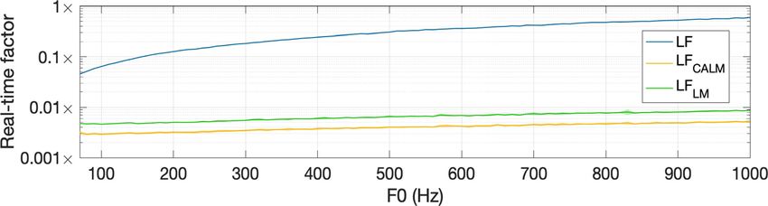
https://doi.org/10.1121/10.0005879

and Degottex et al. (2013): LF model]; or expressive text-                 conducted in Sec. III for assessing the perceptual equiva-
to-speech synthesis [Raitio et al. (2013), Airaksinen et al.               lence of the three models. Armed with analytic formulations
(2016), and Juvela et al. (2019): LF model]. This list is not              and perceptual analyses, the discussion in Sec. IV summa-
exhaustive; however, LF has been the most widely adopted                   rises the results obtained: linear-filter formulations equiva-
model for analysis and synthesis of speech signals.                        lent to the LF model are able to account for both the
     The main limitation of the LF model is its computa-                   observed glottal formant and glottal flow waveforms.
tional complexity. It requires solving implicit equations that
can only be performed with numerical approaches. This                      II. LINEAR-FILTER FORMULATION OF GLOTTAL
model is not suitable for applications where computational                 FLOW MODELS
complexity is a constraint, such as real-time speech or sing-              A. Glottal flow model parameters: LF and Rd
ing synthesis. Also, spectral glottal flow models are desir-
able because voice quality is often described in spectral                        All GFMs attempt to describe a vocal-fold vibration
terms (e.g., voice spectral tilt, brightness, tenseness): spec-            period in time-domain (see Fig. 1). Three phases are consid-
tral parameters are closer to perception than time-domain                  ered: the opening phase (lung pressure forces the vocal folds
parameters. It is therefore interesting to investigate the                 to spread, and an increasing air flow passes through the glot-
apparent discrepancy between GFM like LF and filter                        tis); the closing phase (the elasticity of the vocal folds takes
impulse-response models. Along this line, Doval et al.                     over, closing the air passage); the closed phase (the airflow
(2006) highlighted that LF and the other time-domain mod-                  is blocked). Then the lung pressure increases again, and a
els under study have a simple magnitude representation in                  new opening phase follows. This cycle can be represented
the frequency-domain that can be modelled with a third                     by five parameters (Doval et al., 2006): the cycle period T0
order filter, as also noted by Childers and Lee (1991). This               or fundamental frequency F0 ¼ 1=T0 ; the cycle amplitude,
has led to the proposal of new models: the causal/anti-causal              generally represented by E, the maximum of the absolute
linear model (LFCALM) by Doval et al. (2003), followed by                  value of the glottal flow derivative (GFD) (i.e., the negative
an all-causal linear model (LFLM) used in the Cantor                       peak at the glottal closure instant has amplitude E); the
Digitalis singing synthesiser (Feugère et al., 2017), which               open quotient Oq, the ratio of the open phase duration Te
both gradually simplify the computation of the glottal flow                over the period T0; the asymmetry coefficient am, the ratio
by using digital filters instead of analytic functions, thus               of the opening phase duration Tp over the open phase dura-
enabling a precision-complexity trade-off, LF being the                    tion; and Ta, the closing time duration (Fig. 1). Period T0
most precise and LFLM the simplest. While we will show in                  and amplitude E change the time and amplitude scales of
Sec. II that the simplification operating on LFCALM and                    the glottal flow. The three other parameters change the
LFLM can substantially modify the glottal flow waveform,                   shape of the glottal flow and account for the voice timbre or
it is not clear if this affects their auditory perception. The             quality. Empirically, Fant et al. (1994) established that the
aim of this paper is threefold. Section II studies the three               perceptual effect of the shape parameters Oq, am, and Ta can
models LF, LFCALM, and LFLM in terms of linear filters.                    be gathered into a unique high-level parameter called Re ini-
Formulations for impulse responses are derived, and differ-                tially, Rd afterward (Fant, 1995) (see Appendix A). Typical
ences between the models are investigated. After this objec-               values of Rd range from 0.4 (short open phase, strong asym-
tive and analytic comparison, subjective experiments are                   metry of the glottal flow leading to a tense voice) to 2.7

FIG. 1. Left: Temporal parameters of the LF model on the glottal flow (top) and its derivative (bottom). Right: Spectrum magnitude (top) and phase
(bottom) of the GFD.

1274     J. Acoust. Soc. Am. 150 (2), August 2021                                                                                   Perrotin et al.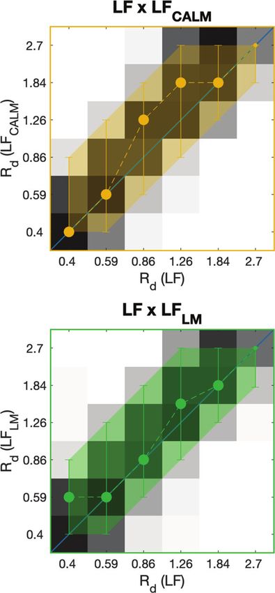
https://doi.org/10.1121/10.0005879

(long open phase, symmetry of the glottal flow providing a             Perrotin and McLoughlin, 2019, 2020). The perceptual effect
relaxed voice). Note that the time-domain NAQ-coefficient              of this phase difference is studied in Sec. III.
proposed later (Alku et al., 2002) is proportional to Rd. Rd                To summarise, the LF model that is widely accepted as
will be used as a control parameter below.                             a precise time-domain GFM has been simplified by a
                                                                       frequency-domain representation that uses a mixed-phase
B. Glottal formant, LFCALM, and LFLM                                   third order filter called LFCALM. To go further in reducing
                                                                       computation complexity, an all-causal linear model (LFLM)
      Radiated sound pressure outside the vocal tract can be
                                                                       has been recently formulated.
approximated by the derivative of the speech flow measured
                                                                            All three GFMs are defined in terms of their open and
at the lips. For this reason, the glottal flow derivative is often
                                                                       closed phase, described separately in Secs. II C and II D. For this
preferred to the glottal flow for analysis purposes. The spec-
                                                                       reason, we define glottal opening instants (GOIs) that mark the
trum of the glottal flow derivative shows a marked spectral
                                                                       beginning of each open phase and are spaced by a duration of T0
peak, the glottal formant. Figure 1 displays on the right the
                                                                       and glottal closure instants (GCIs) marking the beginning of each
magnitude spectrum of the glottal flow derivative computed
                                                                       closed phase. GOIs and GCIs are spaced by a duration of Oq T0 .
with the LF model, superimposed on a third order filter
approximation. Two poles form the glottal formant, a low-              C. Modeling the open phase
frequency resonance with centre frequency Fg that is directly
related to the oscillation of the open phase of the vocal folds.       1. General formulation of the open phase
The remaining pole is an extra attenuation with cut-off fre-               Let us define the impulse response of a truncated second
quency FST, called spectral tilt, that is responsible for the          order filter, whose generic formulation is
smoothness of the closed phase of the vocal folds. Phase

analysis has shown that this third order approximation is a                   hT ðtÞ ¼ Gn ean t sin ðbn t þ /n Þ if t 2 D
mixed-phase model (Gardner and Rao, 1997), allowing it to                                                                        (1)
                                                                              hT ðtÞ ¼ 0                         elsewhere:
represent the open phase of the LF model as a second order
filter response (damped sinusoid) that evolves toward nega-            If hT is anti-causal, T < 0 is the instant of truncation,
tive time, while the closed phase resembles the response of a          D ¼ ½T; 0, and an > 0. Its causal counterpart is defined for T
first order filter (decreasing exponential) that evolves toward        > 0, D ¼ ½0; T, and an < 0. It can be shown that the open
positive time (bottom-left of Fig. 1). Following this analysis,        phase definitions of the three GFMs under study can be formu-
the causal/anti-causal linear model of the glottal flow                lated with respect to Eq. (1) by setting appropriately the Gn, an,
(LFCALM) has been proposed by Doval et al. (2003) to gener-            bn, /n , and T parameters (index n is subsequently replaced by
ate a glottal derivative waveform by filtering a pulse train           the name of the model in consideration: LF, CALM, or LM). In
with the mixed-phase third order filter. The LFCALM is a sim-          their original formulations, LF is defined as a continuous time-
ple formulation reproducing the dual relations between time-           domain function, while LFCALM and LFLM are defined as digital
domain parameters and spectral shape (Gobl et al., 2018;               filters (Z-domain). For the sake of generalisation, all expressions
Henrich et al., 2001). A real-time implementation of the               are given below as equivalent continuous representations (time
model called RT-CALM was then derived by d’Alessandro                  and Laplace domains), and derivation details from the original
et al. (2006). The mixed-phase characteristic of the glottal           papers’ formulations are given in Appendixes B, C, and D.
flow has been exploited for the estimation of the glottal flow
from speech signals (Bozkurt et al., 2005; Drugman et al.,                  a. LF. The LF model (Fant et al., 1985) is defined by an
2011; Hezard et al., 2013). The glottal formant can also be           analytic function in the time-domain relative to the GOI and
represented by causal filters, following Klatt (1980) and              can be interpreted as an unstable, divergent, and truncated
Holmes (1983), but at the expense of some distortion in the            causal filter. However, re-parameterization with Oq and am and
phase spectrum compared to the LF model. A formulation of              setting the time origin at the GCI (see Appendix B) allow us to
this causal linear voice source model LFLM has been pro-               express LF as an anti-causal filter truncated at TLF ¼ Oq T0 ,
posed and used for real-time voice synthesis and voice source          matching Eq. (1). The equations below give the resulting
analysis (Feugère et al., 2017; McLoughlin et al., 2020;              waveform analytic expression and its Laplace transform:

    8
    >
    >                   E                  p        p
    >
    > hLFopen ðtÞ ¼       eaLF t sin            tþ      ; t 2 ½Oq T0 ; 0
    >
    >                     p              am Oq T0    am
    <               sin
                         am                                                                                                            (2)
    >
    >               ð
    >
    >
                      0
                                           GLF bLF ðesTLF  1Þ þ Es
    >                              st
    : HLFopen ðsÞ ¼ T hLFopen ðtÞe dt ¼
    >
                                                ða  sÞ2 þ b2
                                                                     :
                        LF                            LF          LF

One can now identify from the top equation the values of parameters GLF ; aLF ; bLF ; /LF , and TLF that are summarised in
Table I. aLF is the open phase damping coefficient. It is set so that the airflow of a period is zero and results from an implicit
equation (see Appendix B).
J. Acoust. Soc. Am. 150 (2), August 2021                                                                            Perrotin et al.   1275
https://doi.org/10.1121/10.0005879
b. LF CALM . The causal/anti-causal linear model uses a The time-domain response of LFCALM, truncated at
second order anti-causal and truncated bandpass filter to TCALM ¼ Oq T0 , and the frequency-domain response are
model the open phase of the glottis (Doval et al., 2003), given by computing the inverse Z-transform and Laplace
whose equation and parameters are derived in Appendix C. transform of the filter, respectively,
8
>
> E aCALM t p
>
> hCALM ðtÞ ¼ e sin t þ pð1 a m Þ ; t 2 ½Oq T0 ; 0
< open
sin ðpð1 am ÞÞ Oq T0
ð0 (3)
>
> ð1 þ eðaCALM sÞTCALM ÞEs
>
> H ðsÞ ¼ h ðtÞe st
dt ¼ :
: CALM open
TCALM
CALM open
ðaCALM sÞ2 þ b2CALM
We find again the general formulation of Eq. (1), and the LFCALM parameters are summarised in Table I.
c. LF LM . The LFLM model (Feugère et al., 2017) is the causal version of LFCALM with the difference that the filter is
not truncated, since it converges (see Appendix D). The time and frequency responses of LFLM, whose parameters are given
in Table I, are again given by computing the inverse Z-transform and Laplace transform of the filter,
8
>
> E p
>
< hLMopen ðtÞ ¼ eaLM t sin t pð1 am Þ ; t>0
sin ðpð1 am ÞÞ Oq T0
ð1 (4)
>
> st Es
: HLMopen ðsÞ ¼
> hLMopen ðtÞe dt ¼
ða sÞ2 þ b2LM
:
0 LM
2. Comparison between the GFM open phases show a similar denominator with a complex conjugate pole.
This results in 620 dB/decade asymptotes. In particular, all
Figure 2 displays the open phases of LF (blue), LFCALM
(orange), and LFLM (green) for the glottal flows (top-left), Laplace transforms simplify to E/s at high frequencies,
GFDs (bottom-left), and spectrum of the GFD (right), com- resulting in similar asymptotes for the three GFMs. At low
puted with Rd ¼ 1:84 and E ¼ 0.2. The top-right of Fig. 2 frequencies, the asymptotes are shifted between models but
displays similarities between the three models. First, all only from a few dB.
open phases derive from second order filters, as their respec- LF and LFCALM display two more similarities. First,
tive Laplace transforms HLFopen , HCALMopen , and HLMopen all their anti-causality causes the GFD phase to increase (bot-
tom-right of Fig. 2); second, they are both truncated at
t ¼ Oq T0 . The thin dashed curves in the left panels show
TABLE I. GFM parameters and implementations. what would be non-truncated versions of LF and LFCALM. A
direct effect of the truncation is the computation of their
LF LFCALM LFLM
Laplace transform on the interval ½Oq T0 ; 0, which results
bn p p p in the appearance of the term esT in HLFopen and HCALMopen .
am Oq T0 Oq T0 Oq T0 This causes the ripples observed in the LF and LFCALM
an >0 p p
spectra. The main difference between LF and LFCALM is
Oq T0 tan ðpð1 am ÞÞ Oq T0 tan ðpð1 am ÞÞ
/n p pð1 am Þ pð1 am Þ
that the former is parameterized to be class C1 i.e., with a
am continuous GFD at the GOI (Oq T0 ). This parameterization
Gn E E E results in a generic second order filter that is neither low-
sin ð/LF Þ sin ð/CALM Þ sin ð/LM Þ pass nor bandpass, as shown by the numerator of HLFopen . A
T Oq T0 Oq T0 1
consequence is the large lobe around the resonance fre-
Open phase quency of the GFD magnitude spectrum. Conversely,
LFCALM is parameterized to be a bandpass filter, which
Formulation Analytic Filter Filter
allows a reduction of the resonance’s lobewidth but cannot
Causality Anti-causal Anti-causal Causal
Truncation At Oq T0 At Oq T0 No truncation
suppress it completely because of the effect of truncation.
The consequence of the bandpass parameterization is a dis-
Closed phase continuous GFD at the glottal opening instant.
Formulation Analytic Filter Filter
Two differences between LFCALM and LFLM are also
Causality Causal Causal Causal highlighted. The difference of causality is well-displayed by
a vertical symmetry in the time-domain and a horizontal
1276 J. Acoust. Soc. Am. 150 (2), August 2021 Perrotin et al.https://doi.org/10.1121/10.0005879
FIG. 2. (Color online) LF (blue), LFCALM (orange), and LFLM (green) open phases. Left: Glottal flows and their derivatives. Right: Magnitude and phase
spectrum of the glottal flow derivatives.
symmetry of the phase spectrum. Also, because LFLM con- filter attenuating high frequencies above its cut-off frequency
verges, it is not truncated at Oq T0 . This implies a leak of the Fa ¼ 1=ð2pTa Þ and called spectral tilt (Doval et al., 2003;
period to the next one but also greatly simplifies its imple- Feugère et al., 2017). Filter formulation is given in Appendix
mentation. As a result, its spectrum is the exact frequency C. In these cases, the spectral tilt filter is applied on the full
response of a bandpass filter, with no ripples and no lobe signal and therefore changes the open phase shape.
around the resonance centre frequency. Note that the verti-
cal symmetry of the GFD between LFCALM and LFLM 2. Comparison between the GFM closed phases
implies a sign inversion of the glottal flow, but one that the Figure 3 displays the three GFM full waveforms,
ear is not sensitive to. obtained by adding to the open phases of Fig. 2 their respec-
tive closed phase contributions while keeping Rd ¼ 1:84.
D. Modeling the closed phase Note that this process changes the open phases. The top-right
panel shows high similarity between the three GFMs’ spec-
1. Formulation of the closed phases
trum magnitudes. The closed phase adds a supplementary
Definitions of the GFM closed phase fall within two cate- 20 dB/decade attenuation to all open phase spectra, result-
gories (Doval et al., 2006): it is either described in the time- ing in a 40 dB/decade attenuation at high frequencies. We
domain by an analytic formulation, as LF, or defined in the can also observe an increase in gain in low frequencies for
frequency-domain with a first order filter, as LFCALM or LFLM. the LF model. This is directly linked to the change of the aLF
parameter. A consequence is the largest amplitudes of the
a. LF: Analytic expression. The closed phase of the LF glottal flow and glottal flow derivative for LF.
model, after shifting the glottal closing instant at t ¼ 0, is Looking at the phase spectrum (bottom-right panel), LF
expressed as and LFCALM almost overlap, showing a similar effect of the
closed phases on their respective phase spectra: it adds a
E t supplementary p=2 offset at high frequencies to all phase
hLFclosed ðtÞ ¼ ðe eðT0 Oq T0 Þ Þ; t 2 ½0; T0 Oq T0 ;
Ta spectra of the open phases. The spectral tilt filter is dis-
(5) played in black. This offset introduces an asymmetry
where is the closed phase coefficient. It satisfies the conti- between LF and LFCALM on one side and LFLM on the other.
nuity of the open and closed phase expressions at the GCI The addition p=2 at high frequencies for all models
and is obtained from an implicit equation (see Appendix B). reduces the phase of LF and LFCALM from 3p=2 to p but
Note that because aLF is computed from , the shape of the also reduces the phase of LFLM from 3p=2 to 2p. This
open phase depends on the closed phase, although both asymmetry is reflected in the shapes of the glottal flow
phases are defined by distinct analytical expressions. derivatives (bottom-left panel). One can see that LFLM and
LFCALM are not symmetrical anymore and that the filtering
b. LF CALM and LF LM : Filtering. With LFCALM and attenuates more the GFD peak near the glottal closure
LFLM, the closed phase is modelled by a first order low-pass instant for LFLM than for LFCALM. Finally, it is important to
J. Acoust. Soc. Am. 150 (2), August 2021 Perrotin et al. 1277https://doi.org/10.1121/10.0005879
FIG. 3. (Color online) LF (blue), LFCALM (orange), and LFLM (green) waveforms including closed phases. Left: Glottal flows (top) and derivatives (bottom).
Right: Magnitude (top) and phase (bottom) spectrum of the glottal flow derivatives.
mention that the spectral tilt filter is not truncated for and F0 value, we computed the mean and standard deviation
LFCALM and LFLM, and its application results in an infinite of the real-time factor across the six Rd values. The means
response that may overlap with the next period. This appears for each model are represented by the thick coloured lines,
for high values of Rd, as shown in Sec. II F. and the shading around each mean value highlights the
6 standard deviation range around the mean. LFCALM and
E. Assessment of computational costs LFLM are more than 10–100 times faster than LF. This is a
direct consequence of the resolution of the implicit equation
To evaluate the computational efficiency of each GFM,
for the LF model, which is costly. Also, the efficiency of LF
we measured the average time necessary to compute one
decreases with higher F0 because the resolution of the
period of a 1-s stationary signal for each model. The ratio of
implicit equation requires a constant duration. Therefore,
computation time over the period duration gives the real-
when the period duration decreases, the real-time factor
time factor. A real-time factor below 1 means that the signal
increases, and this dependency between computation effi-
is faster to compute than to play back, so we can listen the
ciency and input parameter is not desirable. Finally, Rd has
signal while it is generated. Inversely, a real-time factor
no effect on the computation time for all three GFMs.
higher than 1 indicates that the signal takes longer to com-
pute than to play back. This experiment was made in the
condition of a fine-grain control of the GFM: parameters are F. Summary of the model implementation and effect
of Rd
calculated for each period. To assess the dependency of the
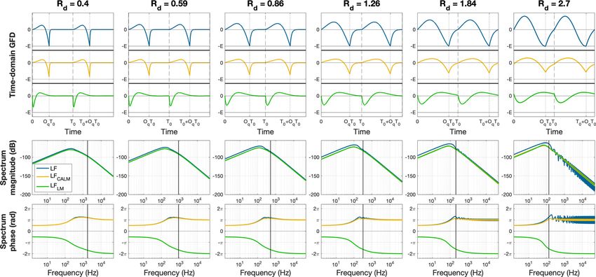
real-time factor on F0 and Rd, we generated 564 stationary Table I summarises the implementations of the three
signals using a combination of the six Rd values described in GFMs under study. To conclude this section, Fig. 5 shows
Sec. III and 94 F0 values, from 70 to 1000 Hz with steps of the effect of Rd on the GFD (top row) and the respective
10 Hz. All signals were generated on an iMac Intel Core i9, spectra computed on a single period (second and third rows)
with a 3.6 GHz processor. Figure 4 displays the real-time for the three models [LF (blue), LFCALM (orange), and
factors for the three GFMs depending on F0. For each model LFLM (green)]. In the top row, the dashed vertical lines
FIG. 4. (Color online) Computational
efficiency of each model expressed in
real-time factor: LF (blue), LFCALM
(orange), and LFLM (green).
1278 J. Acoust. Soc. Am. 150 (2), August 2021 Perrotin et al.https://doi.org/10.1121/10.0005879
FIG. 5. (Color online) Glottal flow derivatives (top row) and their magnitude (second row) and phase (bottom row) spectra computed with the three models
[LF (blue), LFCALM (orange), and LFLM (green)] for a range of Rd values (each column).
represent the GOIs, while the dotted lines show the GCIs. In LFCALM and LFLM. The GFD computed for one period over-
the second and third row, the vertical line indicates the cut- laps on the next one, leading to negative (respectively, posi-
off frequency of the spectral tilt filter. Globally, Rd has a tive) value of the GFD at the GOI for LFCALM (respectively,
similar effect on the three GFMs. Looking at the spectrum LFLM).
magnitude, low values of Rd lead to higher centre frequency We have shown that the difference of construction
and bandwidth of the glottal formant and a higher spectral between the three GFMs (formulation, causality, truncation)
tilt cut-off frequency. These combined effects favour the leads to clear visible differences in the GFD waveforms and
presence of numerous harmonics that give a sharp GFD clo- spectra. However, their effect on auditory perception is
sure, close to the shape of an impulse. This is typical for unclear and is assessed in Sec. III.
tensed and loud voice, when the vocal folds open and close
abruptly. Inversely, high values of Rd lower the centre fre- III. PERCEPTUAL COMPARISON OF VOICE SOURCE
quency and bandwidth of the glottal formant as well as the MODELS
spectral tilt cut-off frequency. It thus emphasises more the
first and second harmonics, leading to a more sine-like GFD A. Experiment
shape. This is lax/soft voice, when the vocal folds oscillate 1. Protocol and task
more symmetrically.
In the first column of Fig. 5, the three GFMs appear The aim of the experiment was to assess any perceptual
very similar for two reasons. First, a low value of Rd leads difference between the three GFMs for different values of
to a high attenuation coefficient an that allows LF and the Rd parameter. We used for this purpose a two-alternative
LFCALM to have almost horizontal tangents at GOI. The forced-choice (2AFC) protocol (Kingdom and Prins, 2016),
truncation thus does not introduce an abrupt change of slope where each subject’s task was to listen to paired sounds and
on the GFD, which results in a reduction of ripples on the to say if they were the same or different, with respect to any
LF and LFCALM spectra. Second, the effect of spectral tilt distinctive features, whatever their nature (e.g., timbre,
that introduces an asymmetry between LFCALM and LFLM is level, pitch, etc.). The experiment was divided into three
small (high cut-off frequency), leading to almost symmetri- blocks. The first block used synthesised sounds from the
cal LFCALM and LFLM GFDs. Inversely, the three GFM GFMs only. The second and third blocks used additional /a/
shapes diverge with increasing values of Rd. Truncation has and /i/ vocal tract models convolved with the GFMs. These
stronger effects on LF and LFCALM, increasing ripples in two vowels were chosen for their lowest (/i/) and highest
their spectrum, and the spectral tilt whose cut-off frequency (/a/) first formant frequency in order to test a more natural
is closed to the glottal formant position has a strong effect vocal sound than the GFM alone.
on the GFD shapes. In particular, one can note that the mini- For each GFM and following Degottex et al. (2013), six
mum values of LFCALM and LFLM diverge from E when values of Rd were chosen equally spaced on a logarithmic
Rd increases. Moreover, the last column illustrates well the scale, leading to three GFMs 6 Rd ¼ 18 stimuli per block
effect of absence of truncation of the spectral tilt filter on (the one displayed on Fig. 5). Then for each block, every
J. Acoust. Soc. Am. 150 (2), August 2021 Perrotin et al. 1279https://doi.org/10.1121/10.0005879
combination of pairs of different GMFs was tested (LFLM B. Results
LFCALM; LFLM LF; LFCALM LF; LFCALM LFLM;
Results report the proportion of pairs that were judged
LF LFLM; LF LFCALM). Finally, 3 vowels 6 pair
similar depending on the factors in consideration. In particu-
combinations 6 Rd values for the first element of the pair
lar, we factorised the six different model pairs into two fac-
6 Rd values for the second element of the pair led to a total
tors: the Model/factor (three levels: LF LFCALM; LFLM
of 648 pairs of stimuli to compare. LF; LFCALM LFLM) and the Order factor that codes the
A computer interface was specially designed for this
order of presentation of each pair (two levels). The addi-
experiment and programmed in MAX 6.1 The protocol was tional factors are Vowel (three levels: source only; /a/; /i/)
identical for all the paired stimuli. To proceed, the subject and Rd (36 levels for all combinations of the six selected
clicked a button, which launched the playback of two values). In the following, we used a single generalised
sounds, A and B, separated by 500 ms. The test sounds were linear model following a binomial distribution to assess the
ordered randomly and played for each subject only once to significance of each factor and their interactions for the per-
keep sessions as short as possible and identical among sub- ception results. The obtained model was subsequently sim-
jects. The subject had to choose whether the two sounds plified by iteratively removing non-significant interactions
were identical or different, without any other choice. Each between factors provided that, at each simplification step,
block lasted approximately 10 min, and subjects were espe- the current and the simplified models do not significantly
cially encouraged to stop and rest between the three blocks differ (p > 0.05) (Crawley, 2013). Post hoc Pearson’s chi-
with a message displayed automatically. The entire experi- squared tests were run to assess whether proportions obtained
ment took place in an acoustically insulated and treated for single conditions significantly differ from chance.
room designed for perceptual experiments. Sound was Figure 6 shows perceptual experiment responses for all
played using a Focusrite (High Wycombe, UK) Scarlett 2i2 factors and interactions except Order (results for both pre-
audio interface on a Mac OSX and AKG (Los Angeles, CA) sentation orders of each pair are merged). The top-left panel
K271 headphones. Before the experiment, subjects were shows results relative to the Rd factor only. Each square cor-
trained with a subset of the sound-pair list (GFM convolved responds to the proportion of pairs judged similar for a given
to /a/ vocal tract or without vocal tract, three Rd values couple of Rd values, all models and Vowels combined. Pairs
spread over the full range of possible values). in black and white were judged similar by 100% and 0% of
A group of 18 subjects took part in the experiment the subjects, respectively. Scores that fall within the red
(median age of 28 years, from 21 to 54 years old). Among rectangle on the colour bar do not significantly differ from
them, 12 subjects worked in the field of sound technologies, chance according to the post hoc Pearson’s chi-squared tests
and six others had a regular musical practice. An audiogram (p > 0.05). On the left-hand side of the figure, the top row
test was performed for each of the subjects, and none of (columns 2–4) shows the model Rd interaction, with all
them reported any known auditory impairment except one levels of Vowel and Order combined; the left column (rows
who was single-side deaf, but stereo listening was not 2–4) shows the Vowel Rd interaction, with all levels of
needed to perform the task. Fourteen subjects were members model and Order combined; the remaining panels show the
of the laboratory and participated in the experiment on a Vowel model Rd interaction for each level of Vowel and
voluntary basis without being paid. The four remaining sub- model, indicated in the top and left margins of the figure.
jects were paid for the experiment. Panels with yellow and green contours are replicated on the
right side, with LF put in the abscissa. On top (respectively,
bottom) for each Rd(LF) value (each column), the distribu-
2. Stimuli specification tion of perceived similar Rd(LFCALM) [respectively,
Stimuli were synthesised at a sampling rate of Fs Rd(LFLM)] values was obtained and superimposed on the
¼ 96 kHz. A constant fundamental frequency of F0 ¼ 110 Hz figure, the circles being the medians and the error bars corre-
and a peak amplitude E ¼ 0.2 were chosen. The LF GFDs sponding to 90% of the values around the median. Smaller
were generated by using the analytic formulations of Eqs. (2) circles indicate scores below the level of significance
and (5) and by solving the implicit Eqs. (B3) and (B4). The (Pearson’s chi-squared test). The shaded area links all error
LFCALM and LFLM GFDs were generated by filtering a pulse bars and represents the space of perceptual equivalence
train with their respective open and closed phase filters between Rd(LF) and Rd(LFCALM) (respectively, Rd(LFLM)).
(Appendix E). All signals lasted 0.3 s, a duration longer than a
standard spoken syllable but short enough to facilitate recall 1. Effect of Rd and order
of the two stimuli for comparison. Fade-in and fade-out ampli- The Rd factor has the strongest effect on results [Rd:
tudes were applied using half Hanning windows of length v2 ¼ 3620, degrees of freedom (df) ¼ 35, p < 0.001]. The
10T0 ¼ 0:09 s. Vowels were invariant in time and were top-left panel of Fig. 6 clearly shows that, over all other fac-
applied by filtering the GFM with a bank of five parallel reso- tors, pairs with similar values of Rd are strongly perceived
nant filters corresponding to vowels /i/ and /a/, whose transfer as similar, and vice versa. This confirms that Rd has a strong
functions are given in Feugère et al. (2017). Finally, all stimuli perceptual effect on the synthesis of glottal flow.
were normalised in dBA.2 Presentation order had no influence on similarity judgment
1280 J. Acoust. Soc. Am. 150 (2), August 2021 Perrotin et al.https://doi.org/10.1121/10.0005879
FIG. 6. (Color online) Perceptual experiment answers. Each square panel shows the percentage of pairs judged similar for every couple of Rd values. Black
and white squares are stimuli judged similar by 100% and 0% of subjects, respectively. See text for a detailed explanation.
(Order: v2 ¼ 0, df ¼ 1, p ¼ 0.90). Therefore, all results dis- (Fig. 5). In particular, subjects judged LF and LFCALM simi-
played in Fig. 6 and detailed below combine the scores of lar mostly when Rd(LFCALM) was greater than or equal to
both presentation orders. Rd(LF). Similarly, LF and LFLM were mostly judged similar
when Rd(LFLM) was greater than to or equal to Rd(LF).
2. Effect of model Conversely, LFCALM and LFLM were judged the most similar
The model factor alone has a small and marginally sig- when they shared the same Rd value, picturing more symmet-
nificant effect on subjects’ scores (model: v2 ¼ 8:8, df ¼ 2, p ric results (top-right panel of the left side of Fig. 6).
¼ 0.012) and therefore demonstrates that the three models The right side of Fig. 6 summarises this asymmetry
are perceptually close to each other. LFCALM and LFLM are between LF and the other models. Recall that these panels
judged the most similar models, and LF and LFLM are judged are replicates of the one with yellow and green contours
the least similar when all answers are averaged. The subjects’ from the left-hand side, but with LF put in the abscissa for
perception seems to reflect the differences between models’ both plots. For each Rd(LF), medians of corresponding dis-
construction that are summarised in Table I. LFCALM and tributions of perceived similar Rd(LFCALM) [respectively,
LFLM derive from the same filtering process, with the only Rd(LFLM)] are all on or above the diagonal. Also, the spread
difference being the causality of the open phase and the trun- of each distribution represented by the error bars (90% of
cation of LFCALM. Inversely, LF and LFLM differ at almost the values around the median) and emphasised by the
every point of Table I. While these results average all possi- shaded areas clearly displays asymmetrical spaces of per-
ble Rd pairs, results depending on Rd follow the significant ceptual equivalence between Rd(LF) and Rd(LFCALM)
two-way interaction between model and Rd (model Rd, [respectively, Rd(LFLM)] that are again above the diagonal,
v2 ¼ 486, df ¼ 70, p < 0.001). Corresponding results are with Rd(LFCALM) [respectively, Rd(LFLM)] mostly equal to
shown in the top row of the left side of Fig. 6 (columns 2–4). or greater than corresponding Rd(LF).
The first observation is that stimuli with similar values of Rd
3. Effect of vowel
are judged extremely similar (close to 100% similarity),
while stimuli with different values of Rd are judged different The effect of vowels (Vowel: v2 ¼ 17:5, df ¼ 2, p
(0% similarity). One can then note a diagonal asymmetry in < 0.001) supports that GFDs presented alone were significantly
the LF LFCALM and LFLM LF panels for Rd values judged less similar than when they were passed through a
higher than 0.86, i.e., when the models start to differ the most vowel, the vowel /i/ giving the highest similarity results.
J. Acoust. Soc. Am. 150 (2), August 2021 Perrotin et al. 1281https://doi.org/10.1121/10.0005879
Therefore, the introduction of resonances in the signal mitigates the waveform and glottal formant as a function of Rd can be
the perception of the glottal source timbre. Moreover, the glottal computed for voice quality analysis and synthesis. As a rule
formant Fg evolves within the range [64, 121] Hz for the chosen of thumb, increasing Rd corresponds to lowering the glottal
values of Rd for all models. The vowel /i/, having its first for- formant centre frequency (often referred to as the “voicing
mant resonance the closest to Fg, could mask the effect of Rd bar” in wideband spectrogram reading) and increasing the
variation, leading to sources judged more similar with /i/ rather spectral tilt toward lower frequencies (the right-hand “skirt”
than vowel /a/. of the glottal formant).
Also, a significant two-way interaction with Rd is pre- Following the proposal of glottal flow models that
sent (Vowel Rd: v2 ¼ 302, df ¼ 70, p < 0.001) as shown attempt to reduce the computational complexity of LF, namely
in the left column of Fig. 6, rows 2–4. Stimuli presented LFCALM and LFLM, we sought to assess the perceptual consis-
with the source only show similarity concentrated around tency of these models. We first showed that even though LF is
the diagonal. When presented with the vowel /i/, the similar- defined from an analytic expression and LFCALM and LFLM
ity spreads across adjacent Rd values for high Rd. This corre- from digital filters, they can all be expressed by the same ana-
sponds to Fg and FST values that are around 100 Hz, close to lytic function, with their own set of parameters. In terms of
the first formant frequency of vowel /i/ (215 Hz). construction, LF and LFCALM have anti-causal and truncated
Conversely, for the /a/ vowel, it seems that stimuli with high open phases, while LFLM has a causal and non-truncated open
Rd value were neither clearly perceived as similar nor dis- phase. The three GFM closed phases are causal.
similar. In this case, the first formant frequency (700 Hz) is Perceptual pairwise-comparison of these models parame-
far above the Fg and FST ranges. A possibility is that sub- terized with various levels of Rd using a same-different
jects either focused on the low or high frequency parts of forced-choice paradigm on short stationary signals shows that
the signal, the former hearing the source differences and the all models are perceived similarly, in that they share the same
latter focusing on the /a/ resonance. Rd parameterization with a possible offset. In particular, LFLM
and LFCALM are perceived similarly with the same Rd, while
4. Remaining interactions LF is perceived similarly as LFCALM and LFLM when LF has
No significant three-way interaction between Vowel and a smaller Rd value. Investigation seems to show that this shift
model and Rd was detected. It can be seen in Fig. 6 that the in perception relates more to the truncation of the glottal flow
trend previously observed in the top row and left column open phase than to a difference of causality. Nevertheless, this
(two-way interactions) applies to the remaining plots. needs to be confirmed in further experiments. Finally, we
Statistical analysis did not reveal a significant Vowel showed that the addition of vocal tract effect with low vocalic
model interaction, showing that the perception of differ- formants increases the perception of similar waveforms when
ences between models is relatively independent from the Rd varies slightly between two waveforms. If the high dissimi-
addition of a vocal tract. Although it would be necessary to larity between waveforms (Fig. 3) has favoured the use of LF
cover a larger number of vocal tract configurations, this for precise analysis of the glottal flow (i.e., time-domain anal-
finding encourages the hypothesis that the choice of the glot- yses), the perceptual consistency between models encourages
tal flow can be made independently from the behavior of the the use of LFCALM and LFLM as simpler models than LF for
vocal tract. Finally, two-way interactions Order Rd and speech synthesis applications and for spectral analyses of the
Order model result from the asymmetry of the model voice source and voice quality.
levels (v2 ¼ 98, df ¼ 35, p < 0.001; v2 ¼ 7:6, df ¼ 2, p
¼ 0.022, respectively). The top row of Fig. 6 showed an
asymmetry between LF and LFCALM and between LFLM and ACKNOWLEDGMENTS
LF. When considering the order of presentation as a factor,
Part of this work has been done in the framework of the
e.g., distinguishing LF LFCALM vs LFCALM LF, the
Agence Nationale de la Recherche, through the ChaNTeR
asymmetry of LFCALM LF results is reversed compared to
and GEPETO Projects (ANR-13-CORD-0011, 2014–2017,
LF LFCALM, hence the two-way interaction.
ANR-19-CE28-0018, 2019–2023) and “Investissements
IV. DISCUSSION AND CONCLUSION
d’avenir” programs ANR-15-IDEX-02 and ANR-11-LABX-
0025-01. The authors are indebted to Professor Boris Doval
In this study, the LF model is reformulated in terms of for his help in the development of the model calculations.
linear filters. This formulation reconciles the apparent dis-
crepancy between time-domain GFM and spectral voice
source models. It allows for quantitative spectral interpreta-
APPENDIX A: HIGH- TO LOW-LEVEL GLOTTAL
tion of the LF model parameters because the correspondence
PARAMETERS
between time-domain and spectral parameters can be analyt-
ically computed. This unifies Fant’s views on the voice Fant (1995) derived a unique high-level parameter Rd to
source: the key point is the interpretation of the LF GFM [in control all low-level parameters Oq, am, and Ta. He first
Fant et al. (1985)] as a mixed phase system and not as a sim- defined intermediate parameters Ra, Rk, and Rg from which
ple resonant filter [as in Fant (1960)]. The joint variation of are derived the low-level parameters,
1282 J. Acoust. Soc. Am. 150 (2), August 2021 Perrotin et al.https://doi.org/10.1121/10.0005879
8
8 > 1 þ Rk b1 z þ b2 z2
> R ¼ ð1 þ 4:8R Þ=100 >
> Oq ¼ HCALMopen ðzÞ ¼ : (C1)
>
>
a d >
> 2Rg 1 þ a1 z þ a2 z2
>
< >
<
Rk ¼ ð22:4 þ 11:8Rd Þ=100
) 1 (A1)
>
> R ð0:5 þ 1:2R Þ >
> am ¼ The associated filter coefficients are those of a second order
>
> k k >
> 1 þ Rk
: Rg ¼ > resonant biquad filter,
0:44Rd 4Ra ð0:5 þ 1:2Rk Þ >:
T ¼R T : a a 0 8
>
> b1 ¼ Ag ;
<
b2 ¼ Ag ;
(C2)
>
> a ¼ 2epBg =Fs cos ð2pFg =Fs Þ;
APPENDIX B: DERIVATION OF LF : 1 2pBg =Fs
a2 ¼ e ;
LF is defined in the time-domain by an analytic func-
tion (Fant et al., 1985). After re-parameterization with Oq where Fs is the sampling frequency and Fg, Bg, and Ag are
and am, Doval et al. (2006) expressed the open phase of the the centre frequency, bandwidth, and amplitude of the reso-
glottal flow derivative as nance (glottal formant) and are defined as
8
EeaLF Oq T0 aLF t p > 1
xLFopen ðtÞ ¼ e sin t ; t 2 ½0; Oq T0 : >
> Fg ¼ ;
p am Oq T0 >
>
sin >
< 2O q T0
am
1 (C3)
(B1) >
> Bg ¼ ;
>
> O T
q 0 tan ðpð1 a m ÞÞ
>
>
Setting the time origin at the glottal closure instant allows : A ¼ E:
g
us to express LF as an anti-causal filter truncated at
TLF ¼ Oq T0 . This is simply done by defining hLFopen ðtÞ By setting aCALM ¼ pBg and bCALM ¼ 2pFg , the time-domain
¼ xLFopen ðt þ Oq T0 Þ, impulse response of LFCALM, truncated at TCA ¼ Oq T0 , is
given by computing the inverse Z-transform,
E p p
hLFopen ðtÞ¼ eaLF t sin tþ ;
p am Oq T0 am E
sin (B2) hCALMopen ðtÞ ¼ eaCALM t
am sin ðpð1 am ÞÞ
t2½Oq T0 ;0:
p
sin t þ pð1 am Þ ;
Oq T 0
Also, if we note XLFopen the Laplace transform of the original for-
mulation given by Eq. (B1), then the time shift operated between t 2 ½Oq T0 ; 0: (C4)
hLFopen and xLFopen is translated as XLFopen ðsÞ ¼ HLFopen ðsÞesOq T0 .
This linear phase shift does not have any effect on the timbre of The LFCALM closed phase causal filter is defined in in
the source and is ignored in this paper. the Z-domain as
aLF is the open phase damping coefficient. It is set so
bST
that the airflow of a period is zero and thus also depends on HST ðzÞ ¼ ; (C5)
the closed phase coefficient [Eq. (5)]. The latter satisfies 1 þ aST z1
the continuity of the open and closed phase expressions
at the GCI from the implicit equation and its filter coefficients are computed from the cut-off fre-
quency Fa ¼ 1=ð2pTa Þ,
1 eðT0 OqT0 Þ ¼ Ta : (B3) (
Given the expression of the closed phase, aLF is calculated bST ¼ 1 e2pFa =Fs ;
(C6)
so that the integral of the glottal flow derivative is null on a aST ¼ e2pFa =Fs :
period, leading to the implicit equation
1
APPENDIX D: DERIVATION OF LFLM
a2LF þ ðp=ðam Oq T0 ÞÞ2
p=ðam Oq T0 Þ p=ðam Oq T0 Þ LFLM is the causal version of LFCALM (Feugère et al.,
eaLF Oq T0 þ aLF 2017). Therefore, the glottal formant, also defined in the
sin ðp=am Þ tan ðp=am Þ
T 0 Oq T 0 1 Z-domain, has the following transfer function:
¼ ðT O T Þ : (B4)
e 0 q 0 1 b1 z1 þ b2 z2
HLMopen ðzÞ ¼ ; (D1)
Both implicit equations are resolved numerically. 1 þ a1 z1 þ a2 z2
whose coefficients are given by Eqs. (C2) and (C3). To have
APPENDIX C: DERIVATION OF LFCALM
a convergent filter, it is necessary that aLM < 0. Therefore,
The LFCALM open phase anti-causal filter is defined in aLM ¼ pBg and bLM ¼ 2pFg . Finally, the time-domain
the Z-domain by Doval et al. (2003) as impulse response of LFLM is
J. Acoust. Soc. Am. 150 (2), August 2021 Perrotin et al. 1283https://doi.org/10.1121/10.0005879
E Burkhardt, F., and Sendlmeier, W. F. (2000). “Verification of acoustical
hLMopen ðtÞ ¼ eaLM t correlates of emotional speech using formant-synthesis,” in Proceedings
sin ðpð1 am ÞÞ
of the ISCA Tutorial and Research Workshop on Speech and Emotion,
p September 5–7, Newcastle, Northern Ireland, UK, pp. 151–156.
sin t pð1 am Þ ; t > 0:
Oq T0 Cabral, J. P., Richmond, K., Yamagishi, J., and Renals, S. (2014). “Glottal
spectral separation for speech synthesis,” IEEE J. Sel. Top. Signal
(D2) Process. 8(2), 195–208.
Childers, D. G. (1995). “Glottal source modeling for voice conversion,”
The spectral tilt filter of LFLM is the same as LFCALM Speech Commun. 16(2), 127–138.
[Eqs. (C5) and (C6)]. Childers, D. G., and Lee, C. K. (1991). “Vocal quality factors: Analysis,
synthesis and perception,” J. Acoust. Soc. Am. 90(5), 2394–2410.
Crawley, M. J. (2013). The R Book, 2nd ed. (Wiley, New York), pp.
628–649.
APPENDIX E: SYNTHESIS WITH LFCALM AND LFLM
d’Alessandro, N., d’Alessandro, C., Le Beux, S., and Doval, B. (2006).
LFCALM open phase uses the anti-causal filter HCALMopen “Real-time CALM synthesizer: New approaches in hands-controlled
voice synthesis,” in Proceedings of the International Conference on New
[Eq. (C1)]. We define a pulse train dgci whose impulses are Interfaces for Musical Expression, June 4–8, Paris, France, pp. 266–271.
placed on the GCIs. The pulse train is then filtered by Degottex, G., Lanchantin, P., Roebel, A., and Rodet, X. (2013). “Mixed
HCALMopen , leading to the recursion equation source model and its adapted vocal tract filter estimate for voice transfor-
mation and synthesis,” Speech Commun. 55(2), 278–294.
xCALMopen ½n ¼ b1 dgci ½n þ 1 þ b2 dgci ½n þ 2 Doval, B., d’Alessandro, C., and Henrich, N. (2003). “The voice source as a
causal/anticausal linear filter,” in Proceedings of the ISCA Tutorial and
a1 xCALMopen ½n þ 1 a2 xCALMopen ½n þ 2 : Research Workshop on Voice Quality: Functions, Analysis and Synthesis,
August 27–29, Geneva, Switzerland, pp. 15–20.
(E1) Doval, B., d’Alessandro, C., and Henrich, N. (2006). “The spectrum of glot-
tal flow models,” Acta Acust. united Acust. 92(6), 1026–1046.
For each period, the impulse response is truncated at the pre- Drugman, T., Bozkurt, B., and Dutoit, T. (2011). “Causal–anticausal
vious GOI. Then the full signal is filtered by the causal spec- decomposition of speech using complex cepstrum for glottal source
estimation,” Speech Commun. 53(6), 855–866.
tral tilt filter HST [Eq. (C5)], leading to the recursion
Fant, G. (1960). Acoustic Theory of Speech Production (Mouton, The
equation Hague, Netherlands), pp. 1–328.
Fant, G. (1995). “The LF-model revisited: Transformations and frequency
xCALM ½n ¼ bST xCALMopen ½n 1 aST xCALM ½n 1: (E2) domain analysis,” Department for Speech, Music and Hearing Quarterly
Progress and Status Report (KTH Computer Science and Communication,
Stockholm, Sweden), Vol. 36, pp. 119–156.
In the case of LFLM, both glottal formant and spectral
Fant, G., Kruckenberg, A., Liljencrants, J., and Bavegard, M. (1994).
tilt filters are applied in their causal form. We define a pulse “Voice source parameters in continuous speech: Transformation of
train dgoi whose impulses are placed on the GOIs. The pulse LF-parameters,” in Proceedings of the International Conference on
train is then filtered successively by the causal version of the Spoken Language Processing, September 18–22, Yokohama, Japan, pp.
1451–1454.
glottal formant filter HLMopen [Eq. (D1)], leading to the recur- Fant, G., Liljencrants, J., and Lin, Q. (1985). “A four-parameter model of
sion equation glottal flow,” Department for Speech, Music and Hearing Quarterly
Progress and Status Report 4 (KTH Computer Science and
xLMopen ½n ¼ b1 dgoi ½n 1 þ b2 dgoi ½n 2 Communication, Stockholm, Sweden), Vol. 26, pp. 1–13.
Feugère, L., d’Alessandro, C., Doval, B., and Perrotin, O. (2017). “Cantor
a1 xLMopen ½n 1 a2 xLMopen ½n 2 ; Digitalis: Chironomic parametric synthesis of singing,” EURASIP J.
(E3) Audio Speech Music Process. 2017, 1.
Fujisaki, H., and Ljungqvist, M. (1986). “Proposal and evaluation of models
for the glottal source waveform,” in Proceedings of the IEEE
and the spectral tilt filter HST [Eq. (C5)], leading to the International Conference on Acoustics, Speech, and Signal Processing,
recursion equation April 7–11, Tokyo, Japan, Vol. 11, pp. 1605–1608.
Gardner, W. R., and Rao, B. D. (1997). “Noncausal all-pole modeling of
xLM ½n ¼ bST xLMopen ½n 1 aST xLM ½n 1: (E4) voiced speech,” IEEE Trans. Speech Audio Process. 5(1), 1–10.
Gobl, C., Murphy, A., Yanushevskaya, I., and Nı Chasaide, A. (2018). “On
the relationship between glottal pulse shape and its spectrum:
1 Correlations of open quotient, pulse skew and peak flow with source har-
http://cycling74.com (Last viewed 8/16/2021).
2 monic amplitudes,” in Proceedings of Interspeech, September 2–6,
See the supplementary material https://www.scitation.org/doi/suppl/
Hyderabad, India, pp. 222–226.
10.1121/10.0005879 for all stimuli.
Gobl, C., and Nı Chasaide, A. (2003). “The role of voice quality in commu-
nicating emotion, mood and attitude,” Speech Commun. 40(1), 189–212.
Hedelin, P. (1984). “A glottal LPC-vocoder,” in Proceedings of the IEEE
Airaksinen, M., Bollepalli, B., Juvela, L., Wu, Z., King, S., and Alku, P. International Conference on Acoustics, Speech, and Signal Processing,
(2016). “GlottDNN—A full-band glottal vocoder for statistical parametric March 19–21, San Diego, CA, pp. 21–24.
speech synthesis,” in Proceedings of Interspeech, September 8–12, San Henrich, N., d’Alessandro, C., and Doval, B. (2001). “Spectral correlates of
Francisco, CA, pp. 2473–2477. voice open quotient and glottal flow asymmetry: Theory, limits and exper-
Alku, P., B€ackstr€om, T., and Vilkman, E. (2002). “Normalized amplitude imental data,” in Proceedings of Eurospeech, September 3–7, Aalborg,
quotient for parametrization of the glottal flow,” J. Acoust. Soc. Am. Denmark, pp. 47–50.
112(2), 701–710. Hezard, T., Helie, T., and Doval, B. (2013). “A source-filter separation
Bozkurt, B., Doval, B., d’Alessandro, C., and Dutoit, T. (2005). “Zeros of algorithm for voiced sounds based on an exact anticausal/causal pole
Z-transform representation with application to source-filter separation in decomposition for the class of periodic signals,” in Proceedings of
speech,” IEEE Signal Process. Lett. 12(4), 344–347. Interspeech, August 25–29, Lyon, France, pp. 54–58.
1284 J. Acoust. Soc. Am. 150 (2), August 2021 Perrotin et al.https://doi.org/10.1121/10.0005879
Holmes, J. (1983). “Formant synthesizers: Cascade or parallel?,” Speech features in accentuation,” in Proceedings of Interspeech, August 25–29,
Commun. 2(4), 251–273. Lyon, France, pp. 3527–3531.
Juvela, L., Bollepalli, B., Tsiaras, V., and Alku, P. (2019). “GlotNet—A raw Patel, S., Scherer, K. R., Bj€
orkner, E., and Sundberg, J. (2011). “Mapping
waveform model for the glottal excitation in statistical parametric speech syn- emotions into acoustic space: The role of voice production,” Biol.
thesis,” IEEE/ACM Trans. Audio Speech Lang. Process. 27(6), 1019–1030. Psychol. 87(1), 93–98.
Kingdom, F., and Prins, N. (2016). Psychophysics: A Practical Introduction Perrotin, O., and McLoughlin, I. (2019). “GFM-Voc: A real-time voice
(Academic, Cambridge, MA), pp. 1–346. quality modification system,” in Proceedings of Interspeech, September
Klatt, D. H. (1980). “Software for a cascade/parallel formant synthesizer,” 15–19, Graz, Austria, pp. 3685–3686.
J. Acoust. Soc. Am. 67(3), 971–995. Perrotin, O., and McLoughlin, I. V. (2020). “Glottal flow synthesis for
Klatt, D. H., and Klatt, L. C. (1990). “Analysis, synthesis, and perception of whisper-to-speech conversion,” IEEE/ACM Trans. Audio Speech Lang.
voice quality variations among female and male talkers,” J. Acoust. Soc. Process. 28, 889–900.
Am. 87(2), 820–857. Raitio, T., Suni, A., Vainio, M., and Alku, P. (2013). “Comparing glottal-
Markel, J. E., and Gray, A. H. (1982). Linear Prediction of Speech flow-excited statistical parametric speech synthesis methods,” in
(Springer-Verlag, Berlin), pp. 1–290. Proceedings of the IEEE International Conference on Acoustics, Speech,
McLoughlin, I. V., Perrotin, O., Sharifzadeh, H., Allen, J., and Song, Y. and Signal Processing, May 26–31, Vancouver, Canada, pp. 7830–7834.
(2020). “Automated assessment of glottal dysfunction through unified Rosenberg, A. E. (1971). “Effect of glottal pulse shape on the quality of nat-
acoustic voice analysis,” J. Voice, published online. ural vowels,” J. Acoust. Soc. Am. 49(2B), 538–590.
Nı Chasaide, A., Yanushevskaya, I., Kane, J., and Gobl, C. (2013). “The Veldhuis, R. (1998). “A computationally efficient alternative for the LF model
voice prominence hypothesis: The interplay of F0 and voice source and its perceptual evaluation,” J. Acoust. Soc. Am. 103(1), 566–571.
J. Acoust. Soc. Am. 150 (2), August 2021 Perrotin et al. 1285You can also read