Scheduling the Main Professional Football League of Argentina
←
→
Page content transcription
If your browser does not render page correctly, please read the page content below
Scheduling the Main Professional Football League of
                     Argentina
                                      Guillermo Durán, Facundo Gutiérrez
         Department of Mathematics and Calculus Institute, University of Buenos Aires, email: gduran@dm.uba.ar,
                                             facumgutierrez@gmail.com

                                                   Mario Guajardo
  Department of Business and Management Science, NHH Norwegian School of Economics, email: mario.guajardo@nhh.no

                                                   Javier Marenco
                     Sciences Institute, University of General Sarmiento, email: jmarenco@ungs.edu.ar

                                         Denis Sauré, Gonzalo Zamorano
     Department of Industrial Engineering, University of Chile, email: dsaure@dii.uchile.cl, gonzaloz@dii.uchile.cl

     In this paper we describe our efforts scheduling Argentina’s First Division professional football league, a.k.a.,
     the Superliga. Following existing work in sports scheduling, we develop an integer programming model for
     the Superliga fixture, which we solve using a decomposition approach. Unlike prior work, such a scheme is
     based on the creation and assignment of cluster patterns, which take advantage of the model’s geographically-
     driven handling of sporting fairness. In addition, we also model the assignment of matches to specific dates
     and time slots, this while considering various aspects pertaining broadcasting networks, the government, and
     international competitions. Our work has been implemented in practice to schedule the 2018-19 and 2019-20
     seasons of the league, improving greatly in a number of criteria over the previous approach. In particular,
     our fixtures have greatly improved sporting fairness, on various tangible dimensions.

     Key words : Combinatorial Optimization, Sports Scheduling, Integer Programming, Decomposition
       Schemes.

1.     Introduction
Background. Argentina’s First Division league is among the most watched professional sport
competitions in the world. The almost 100 year-old competition is constantly ranked among the
most important, most competitive football leagues, home of the highest number of Libertadores’s
cup champions (25, followed by Brazil with 19), and host of some of the most fiercest, most followed
rivalries in professional sports. It is among the highest grossing football competitions in the world, in
terms of GDP-adjusted revenue (shortly behind England’s Premier League, Germany’s Bundesliga,
Spain’s La Liga, and Italy’s Serie A), and birth-place of some of the best players in history. In
Argentina, football is as important as religion (ask the Pope).
  In 2014, the Argentine Football Association (AFA), institution overseeing professional football in
Argentina, changed the format of the First Division tournament, and the number of teams compet-
ing went up from 20 to 30 (10 teams were promoted from the Second Division). After that, teams

                                                            1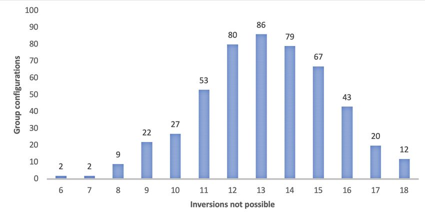
2 Durán et al: Scheduling Argentina’s Superliga
were gradually relegated to the Second Division each year. Starting in 2017, AFA delegated the
management of the First Division tournament to an independent entity called Superliga Argentina
de Fútbol (SAF), and renamed the competition homonymously. In the 2017-18 season, the first
tournament under SAF’s supervision, 28 teams competed in a single round robin (i.e., every team
played against each other once).
SAF faced several challenges in producing a fixture (and afterwards, assigning dates to matches)
meeting sporting fairness and other important criteria. For example, the location of the teams’ home
venues (see Figure 1) and the single round robin format made it possible that the total distance
traveled during a season vary significantly from team to team. (Argentina is the 8th largest country
in the world, so that a match may require a team to travel as much as 3,300 kilometres or 2,050
miles.) Also, because of the significant home-advantage effect in football (see, e.g. Pollard (2006)),
and the heterogeneity among teams in terms of strength/fan-base, a team’s chances of winning the
championship might vary significantly depending on how match venues are assigned. The focus on
sporting fairness is a goal in and of itself, as it also translates into -or needs to be balanced with -
economic fairness. In this regard, there are substantial economic rewards associated with claiming
a championship and qualifying to international cups (CONMEBOL’s Copa Libertadores and Copa
Sudamericana), ticket sales for high attendance games (usually against strong teams) constitute a
significant source of revenue, specially for smaller teams.
In this context, considering our experience in scheduling professional football leagues (Alarcón
et al. 2017), SAF’s management contacted our research group, seeking help in preparing a fixture
for the 2018-19 season, which ought to feature 26 competing teams. As is traditionally the case
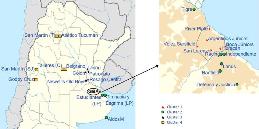
Figure 1 Locations of the 2018-19 SAF teams. Left panel: teams outside the Greater Buenos Aires (GBA) area.
Right panel: teams in the GBA areaDurán et al: Scheduling Argentina’s Superliga 3 in professional leagues that use the single round robin format, the tournament’s fixture ought to consider 25 rounds, with each round spanning three to four consecutive days (e.g. from Friday to Monday), and each team playing exactly once on each round. The dates of each round were fixed in advance, so as to accommodate, for example, the international FIFA calendar, so that the tournament spanned from August 2018 to April 2019. A feasible schedule must then specify when (at which time, on which day, of which round) any two teams face each other, and on whose venue. Sporting Fairness. Our work began with an analysis of fixtures for previous tournaments, in terms of sporting fairness and potential legacy issues. This allowed us to identify key aspects that SAF would like to prioritize in a fixture. Prior to the 2018-19 season, First Division tournaments where scheduled manually, with little attention being paid to sporting fairness. As a result, matches between some pairs of teams took place on the same venue for up to six consecutive tournaments. Overall, from all 325 team pairings, matches between 146 of such pairs had been held in the same venue for two or more consecutive times. The situation was specially dire for some small teams that did not get to play at home against the most popular teams (when the highest ticket revenues are expected) in many consecutive seasons. Take for example the match between River Plate and Banfield : prior to the 2018-19 season, such a match was held six consecutive times at River-Plate’s home venue, which was financially detrimental towards Banfield (River Plate usually has the highest average attendance per game, roughly 48K during the 2018-19 season, while the league average attendance was approximately 20K). In addition, some teams had to travel much more than others during a season, which is detri- mental to sport fairness due to the negative effects associated with travel fatigue (see, e.g. Lastella et al. (2019)). Consider, for example, the situation of two teams from Buenos Aires City: the total traveled distance for Huracán during the season 2017-18 was about 9.9K km while that for Boca Juniors was about 4.5K km. Note, however, that balancing total traveled distances among teams does not necessarily translate into sporting fairness, since teams are not uniformly spaced geographically speaking: when a large number of teams is clustered in a small region and some others are far from such a region, and each other, then some teams will inevitably have to travel considerably more than the others. Conversely, if sporting fairness is to be preserved, one would do expect to see teams that are in the same geographical region traveling comparable total distances. This is particularly the case for the strong teams from Buenos Aires City: a schedule where their traveled distances differ by too much is certain to draw criticism from managers, players, fans, and the media. The scheduling problem faced by SAF was further complicated by a number of requirements either negotiated by the television networks owning the tournament’s broadcasting rights, or imposed by the government. For example, matches gathering fans from the fiercest rivalries deserve
4                                                               Durán et al: Scheduling Argentina’s Superliga

special consideration, not only because of the hype they generate, but also due to their implications
to public order. For a recent, rather infamous example, recall the final of the 2018 Libertadores
Cup, dubbed “the final to end all finals” (Smith 2018), which ought to consist on a two-legged
tie between Boca Juniors and River Plate; such final had the second leg played in neutral ground
(Madrid) due to major public disorders caused by fans in Buenos Aires.
    Additional considerations include stadium availability, constraints on facing strong teams con-
secutively, and constraints on consecutive games with the same home-away status. We review all
these considerations in Section 2, where we outline a model for the SAF fixture.
Objective and Methodology. Our work aimed at developing a framework for helping the SAF
create a fixture for the First Division tournament, that complied with the various criteria for
sporting fairness and with those raised by the various stakeholders (clubs, broadcasting network,
government, etc.). Because creating such a fixture is in practice a highly iterative procedure, where
proposal solutions are produced, revised and new criteria raised, core to our approach is an algo-
rithm capable of quickly producing candidate fixtures. Following existing work in sports scheduling,
we developed an Integer Programming (IP) model for a fixture (see, e.g. Rasmussen and Trick
(2008), Wright (2009), Kendall et al. (2010), Ribeiro (2012), and Van Bulck et al. (2020) for sur-
veys and literature classifications on the subject). Such a model, which we present in Section 2,
could not be solved directly by commercial solvers (they not only improved slowly on the objective
value and best known bound, but also failed in finding feasible solutions after days of running, in
some instances), a situation that is rather common in the sports scheduling literature. In order to
find approximate solutions to the aforementioned model, we used a decomposition scheme where:
first, we partition clubs into geographically driven clusters (which we use to balance total traveled
distances); then we generate a set of cluster patterns, each of which, when assigned to a team,
indicates the rounds and the cluster of the rivals where it has to play as visitor over the tourna-
ment; finally, we solve a version of the fixture model where cluster patterns are assigned to teams,
and a fixture is formed. Once a fixture assigning matches to rounds is created, we solve a separate
problem, assigning matches to specific days and times within each round.
Contribution and Literature Review. Our work contributes to a growing list of applications of
IP to scheduling professional football. Leagues in Holland (Schreuder 1992), Austria and Germany
(Bartsch et al. 2006), Chile (Durán et al. 2007, 2012, Alarcón et al. 2017), Denmark (Rasmussen
2008), Belgium (Goossens and Spieksma 2009), Norway (Flatberg et al. 2009), Honduras (Fiallos
et al. 2010), Brazil (Ribeiro and Urrutia 2012), and Ecuador (Recalde et al. 2013), have been
scheduled using similar techniques. Recently, Duran et al. (2017) used IP to schedule the World
Cup qualifiers in South America. Although all these references have greatly contributed to improve
the scheduling practice in the particular competitions they arise, Van Bulck et al. (2020) argue
Durán et al: Scheduling Argentina’s Superliga 5 that rather few general insights have been gained from previous studies, which poses an obstacle to the algorithmic progress in the area. A first contribution of our work relates to the geographical clustering of the teams. Unlike most of the previous sports scheduling literature, which has focused on minimizing the total distance traveled by the teams (this is, for example, the objective function of the Traveling Tournament Problem (TTP), a seminal work by Easton et al. (2001)), our focus is on balancing the amount of similar trips made by comparable teams (in terms of their location). This approach, which provides a better fit with how clubs perceive travel, still produces fixtures where the traveled distances of teams within a same cluster are similar to each other, and, more importantly, is deemed as fair by team managers and the SAF alike. A second contribution relates to the use of cluster patterns within our decomposition scheme. While such schemes are a commonplace in the sport scheduling literature, most are based in the creation and use of home-away patterns, which, once assigned to a team, indicates whether such a team plays at home or not on each round; see Nemhauser and Trick (1998) for a pioneer application, and Rasmussen and Trick (2008) for a detailed survey on the use of such patterns. Our approach instead exploits the generation of geographical clusters, to implement a heuristic approach based on cluster patterns, which significantly reduces the number of variables needed to form a candidate schedule. Note that, while cluster patterns in our work are driven by geography, the approach is flexible as to, in general, incorporate other clustering criteria (see Section 8 for further details). As expected, the approach helped us to obtain high-quality solutions in a matter of seconds or few minutes, and even optimal solutions in some instances. A third contribution consists in the use of IP techniques to perform the final assignment of specific dates and times to matches, pursuing sporting fairness criteria. In this regard, while the tournament schedule is made public before the tournament begins, the exact day/times of each match might be assigned closer to the beginning of each round. Prior to the 2018-19 season, exact day/times were assigned manually round by round (thus, only 13 matches were assigned at each time). Such a manual and myopic approach could barely incorporate concerns raised by the broadcasting network, teams playing international tournaments, and other important economic and sporting fairness factors. For example, recent empirical research by Goller and Krumer (2020) has shown that games that take place on weekdays have not only a lower attendance than games played during weekends, but also convey significantly lower home advantage for the underdog teams. Thus, in general, teams prefer to play on Saturdays/Sundays rather than on Fridays/Mondays. Through our modelling approach, we are able to consider these concerns and perform the assignment of games to day and times simultaneously for multiple rounds. This application, to the best of our knowledge, has not been considered so far in the literature.
6                                                               Durán et al: Scheduling Argentina’s Superliga

Organization of the paper. The rest of the paper is organized as follows. Section 2 presents an
IP formulation to creating a fixture for the SAF tournament. Then, Sections 3 and 4 detail the
creation of geographical clusters and patterns, as well as their use in finding candidate fixtures.
Section 5 presents our model for assigning day/times to matches in the fixture. Sections 6 and 7
present our results and a summary of our further collaboration with SAF, respectively. Finally,
Section 8 presents our closing remarks. The details and mathematical formulations of the models
used in this work are relegated to Appendices A to D.

2.     An IP model for the SAF Fixture
Next, we describe a series of conditions that ought to be met by a feasible fixture for the 2018-19
season of the SAF. Such requirements are encoded into an IP formulation, which is presented in full
in Appendix A. Here, we provide a qualitative description of such requirements. Note that these
requirements do not consider the assignment of matches to specific date/times within a round, as
those are solved afterwards by the model described in Section 5.
Logical & traditional requirements. A first set of requirements is to comply with the single
round robin format. That is, each team plays once on each round, and every pair of teams plays
once during the tournament. Also, teams were to play at home on at least 12 (at most 13) rounds. In
this regard, we also limit the number of breaks that a team may experience during the tournament
(a break occurs when a team plays on two consecutive rounds with the same home/away status).
In particular, we limit the number of both home and away breaks to at most one per team, which
could not occur on neither the first nor the last rounds.
Matches against strong teams. As in many leagues in the world, there are few teams in the
SAF which are regarded, by consensus, as stronger than the rest, in terms of their fan-base, budget,
and/or historical performance in the tournament (e.g. number of titles). These teams are River
Plate, Boca Juniors, Independiente, Racing Club, and last but not least, San Lorenzo. Because of
the additional pressure experienced when facing a traditionally stronger rival (such matches receive
relative larger attention by fans and the media), smaller teams prefer to balance such matches
throughout the tournament. Also, because of the larger attendances associated with such games,
managers prefer to play at home against such teams. Players also prefer to play at home rather
than, against even larger odds, at the rivals’ turfs.
    Considering the above, we require that no team would face any two strong teams in consecutive
rounds. Also, we require for each team, a minimum number of matches against strong teams to be
played on predefined stages of the tournament (typically, each third or each half of the tournament).
Furthermore, we require that each team would play at home against strong teams at least twice.
In particular, for the strong teams, we impose that they play exactly twice at home against other
strong teams.
Durán et al: Scheduling Argentina’s Superliga 7 Traditional rivalries. In addition to the infamous rivalry between River Plate and Boca Juniors, there is a number of pairs of teams whose match-ups are highly anticipated by the fans (the so- called clásicos). This is the case, for example, of the match between Independiente and Racing Club (both strong teams). Such games are typically followed not only by the fans of such teams, but also by the whole country. For this reason, we require that no two of such games are played on the same round, so as to spread them throughout the tournament. Also, there are a number of rounds on which no such match could be played (e.g. election days, first and final rounds, etc.). In addition, because of the additional stress put on some teams, we impose that no team could play against the traditionally stronger teams in the league (namely, River Plate and Boca Juniors) or their traditional rival in two consecutive rounds. A side-effect of the aforementioned rivalries is the occurrence of football-related violence when- ever clusters of hooligans from rivals teams clash on the streets. This is a major concern for SAF management: just in 2018, there were 10 football-related deaths. In response, the government and AFA put in place mitigating measures such as banning attendance of away fans to matches. While such a measure has been lifted in recent years, it remains in place for fans of all strong teams. So as to collaborate with the effort to eradicate football-related violence, we require that no two rival teams whose home venues are in proximity to each other play both at home on any given round. International Competitions. By the beginning of the 2018-19 season, six SAF teams were scheduled to participate in the 2019 editions of either the Libertadores or Sudamericana cups. Such international competitions are typically played during weekdays (Tuesday to Thursdays), and involve long distance travel. Because of the negative effect of travel fatigue on performance, the SAF aimed at helping these teams to perform well in these competitions by limiting long distance travel on the domestic league, on rounds immediately before international cups’ match-days. Sporting fairness: travel balance. As mentioned in Section 1, because of the geographical distribution of SAF teams, unbalance on total traveled distance is expected, and even desired if one is to maintain sporting fairness. From Figure 1, we see that teams such as San Martı́n or Atlético Tucumán will unavoidably travel longer distances than, say, Hurácan (located in the Buenos Aires area, together with many other teams). In this regard, we seek to promote sporting fairness by balancing total traveled distance among teams in comparable situations (geographically speaking). For this, we considered a partition of SAF teams into clusters, so that total traveled distance is to be balanced among teams within the same cluster. Thus, such a partition ought to cluster teams geographically. In the next section, we discuss the procedure for creating such clusters. Given a set of clusters, we require that each team within a cluster play away against approximately half of the teams on every other cluster. We preferred this criterion over balancing the total distance traveled among teams within a cluster. This, because it has proved to be more efficient computationally
8                                                                Durán et al: Scheduling Argentina’s Superliga

speaking (Durán et al. 2020), and also given that ultimately distance is not the main driver of
sporting unfairness, but rather the hassle related to the travel itself.
Legacy related constraints: status inversion. By the end of the 2017-18 season, 146 pairs of
teams out of the 325 possible had their matches scheduled on the same venue in the last 2 to 6
consecutive occasions. This was a situation that teams, the media and fans alike were quite aware
of, and source of constant criticism. While ideally a new fixture ought to invert the location of all
matches, relative to the 2017-18 season, this proved infeasible due to a number of constraints (for
example, the requirement that each team faced at least two strong teams at home) and variations
in the set of competing teams from one season to the next (due to promotion/relegation rules).
Considering the above, we approached this issue by penalizing all status inversions (among the
aforementioned 146 matches) that would not take place in the objective function.

3.     Teams clustering
As mentioned in Section 1, because teams are not uniformly spaced geographically speaking, bal-
ancing total traveled distances among teams does not necessarily translate into sporting fairness.
Thus, if sporting fairness is to be preserved, one would do expect to see teams that are in the same
geographical region traveling comparable total distances. To address this issue, the model described
in the previous section takes as input a partition of the set of participating teams into clusters,
so that teams on a same cluster are considered to be in comparable situations, geographically
speaking. The model then balances travel of similar teams into the various clusters (for example,
it imposes lower and upper bounds on the minimum and maximum number of trips made by a
team to other clusters). Next, we describe our approach to creating such a partition.
    We first explored the idea of balancing travel through the definition of clusters when helping SAF
scheduling the Argentine youth leagues, where each participating club competes on six different
categories, and thus, with six different rosters. Motivated by balancing the distances traveled by
the rosters of a same club, geographical clusters were formed manually and then used to spread
travel to the different clusters evenly among the club’s rosters. The resulting fixtures managed to
balance travel not only across the rosters of a same club, but also across teams in a same category.
The approach, which proved to be more efficient than attempting to balance distance traveled
directly, was widely accepted by SAF managers (see Durán et al. (2020) for more details).
    In scheduling the Superliga, we refined the approach so as to balance the total distance traveled
by teams on a same cluster. Central to the approach was providing managers with a more for-
mal methodology to generating the team clusters. In this regard, an initial proposal consisted on
considering the administrative organization areas of the country. However, while such a proposal
provided a clear grouping of the teams around Buenos Aires City, it turned less clear how to group
Durán et al: Scheduling Argentina’s Superliga 9 the teams outside this area. Instead, we formulated and solved an IP model that receives as input the desired number of clusters and the distances between the venues of each pair of teams, and provides as output an optimal cluster configuration. The optimality criterion in this model is based on the notion of within-cluster distance, defined for each cluster as the maximum across teams in the cluster of the sum of the distance between the teams’ home venue and the venues of every other team in the cluster. The clustering model focuses on minimizing of the sum of the within-cluster distances, across clusters. The formulation of the model is presented in Appendix B. We solved the model for various values for the number of clusters (the model is solved in a few seconds by commercial solvers), from which SAF chose the option that liked the most. The chosen solution contains four clusters, as depicted in Figure 1. The chosen clusters effectively provided a partition, where teams of a same cluster are similar to each other in the sense of geographical proximity (i.e. small within-cluster distance), and teams from different clusters are relatively apart from each other. 4. Solving the SAF Fixture via Cluster Patterns Considering the criteria introduced in the two previous sections, the IP model formulation for the SAF fixture consisted of roughly 17,500 variables and 5,500 constraints, and could not be solved in reasonable time by commercial solvers such as Cplex (IBM ILOG 2020) or Gurobi (GUROBI 2020). In some instances, the solvers would find a feasible solution after hours of running but then struggled to make further progress after running for days. (In other instances, not even a feasible solution would be found after days.) This is commonplace in the sports scheduling literature, where most problems have proved to be very hard to solve. To illustrate this point, consider that despite the efforts of the research community, the most classic instances of the TTP (introduced about two decades ago by Easton et al. (2001)) still remain unsolved when the number of teams is above ten. As most leagues consist of more than ten teams, it is common in the literature to approach sports scheduling problems using decomposition schemes. The most popular one consists on first solving a sub-problem that generates feasible sets of home-away patterns, and then solving a second one in order to assign these patterns to specific teams, while finding a feasible schedule (a detailed explanation can be found in Rasmussen and Trick (2008)). Because of the challenges encountered when attempting to solve the IP model of Section 2 (even by using the traditional home-away pattern decomposition, which could run for hours before finding an initial solution), we developed an alternative pattern-based decomposition scheme, which allowed us to quickly generate approximate optimal solutions. The decomposition approach is based on cluster patterns. When assigned to a team, a cluster pattern indicates on which cluster should a team play in each round of the tournament. For example, consider pattern (H, A1 , H, A2 , . . .): a
10                                                                 Durán et al: Scheduling Argentina’s Superliga

team which gets this pattern assigned must play a home game in the first round, an away game
against a team of cluster A1 in the second round, a home game in the third round, an away game
against a team of cluster A2 in the fourth round, etc. More formally, we define a cluster pattern as
a tuple whose dimension equals the number of rounds of the tournament and whose elements may
take the value H (for a home match) or a value in the set of clusters.
     The decomposition approach works as follows. On a first step, a set of feasible cluster patterns are
generated and assigned to each team. Then, a modified version of the original IP model of Section
2, incorporating pattern assignments, is used to generate a fixture (see the details in Appendix
C.2). On the bright side, this approach ought to significantly reduce the running time of the latter
model. On the other side, the quality of the fixture created depends on the patterns generated,
so in general optimality is not guaranteed. Moreover, the patterns generated might result in an
infeasible modified model, whereas the original model is feasible.
     To create the cluster patterns, we formulate an IP model that considers the logical and tradi-
tional requirements imposed on the fixture problem, plus some of those referring to traditional
rivalries and travel balance. The formulation of the model can be found in Appendix C.1. An alter-
native approach to pattern generation consists on simply retrieving them from a feasible solution
(obtained, e.g., by the original IP model). Note that every candidate schedule inherently contains
a set of cluster patterns. This approach is of course feasible only after an initial candidate fixture
is available, which was not always the case.
     Incorporating pattern assignments greatly improves our ability to approximately solve the IP
model of Section 2. Consider that, the set of teams to whom a team can be paired against on
any given round is determined by the teams’ assigned pattern. Equivalently, any pair of teams can
only play against each other on rounds where their cluster patterns locate them both at the same
cluster, which ought to coincide with one of the teams’ clusters. This eliminates a considerable
number of decision variables.
     As mentioned, the process outlined above is heuristic and, therefore, is not guaranteed to reach
an optimal solution. Moreover, not any set of patterns constructed in the first stage of the process
outlined above results in a feasible modified IP model. To see this, note that the fixture model
considers constraints which are not present in the pattern generation process. In practice, if a given
set of patterns rendered the (modified) fixture model infeasible, we simply solved the pattern-
generating model again, to quickly find a new set of patterns. Note that, when using patterns from
a feasible fixture (i.e., the alternative approach outlined above), feasibility is guaranteed, and the
modified IP model attempts to improving upon the incumbent (feasible) solution. Alternatively,
one might choose to fix the cluster patterns for a subset of teams, while relaxing the other ones
(a natural choice for this approach is, for example, to fix the cluster patterns of all teams within
Durán et al: Scheduling Argentina’s Superliga 11 a cluster). In practice, using cluster-based patterns helped us to obtain high-quality solutions in a matter of seconds /minutes, and even optimal solutions in some instances (which we know by comparing solutions against the LP relaxation of the original IP model). Note that, while in our work cluster generation is driven by geography, the approach is flexible enough as to incorporate other general clustering criteria. See the discussion in Section 8. 5. Scheduling games to exact days and times Once matches have been assigned to rounds, we solved the problem of assigning matches to spe- cific days and times within each round. This problem, to the best of our knowledge, has not been explored in the sports scheduling literature. Assigning dates and times to matches require incor- porating concerns emanating from various stakeholders (broadcasters, the government, SAF, AFA, to name a few). We developed an IP formulation to conduct such an assignment. The details of the model can be found in Appendix D. Next, we revise the main constraints considered in such a formulation. Security-based considerations. In addition to those security-based constraints imposed in the fixture, we avoid scheduling matches during the same day in venues relatively close to each other. This aims at mitigating the risk of clashes between fans of rival teams (which, unfortunately, in the past have led to violence). Security concerns in Buenos Aires City go even further, as local authorities do not allow more than two matches to be played on a same day. The reasons, beyond public safety, are that, doing it so, would require allocating scarce police resources to overseeing the matches’ venues, and would result in abnormal congestion in public transportation. Considering the above, and the importance assigned by SAF and local authorities to the matter, our objective function attempts (in part) to maximize the number of days on which at most one match is played across Buenos Aires City. Broadcasting considerations. A second set of considerations pertained the two networks who owned SAF broadcasting rights for the 2018-19 season. In this regard, assignment of matches to broadcasters is negotiated with SAF well in advance and serves as an input to our problem, which has a significant impact into feasible day and time assignments. On the one hand, matches to be aired by a same broadcaster can not be assigned to overlapping time-slots during a same day. Moreover, the extent of permissible time separation between matches aired by a same broadcaster should allow conducting all logistics associated with broadcasting a game (setting equipment, allocating staff, etc.), in addition to leaving enough room for airing pre- and post-match content. Also, broadcasters are interested in assigning the most attractive matches on any round to the set of prime-time slots (à la NFL’s Sunday Night Football). Pursuing this goal, we incorporate such an aspect on the objective function, when we attempt to maximize the allocation of these most attractive games (as defined by the networks) to prime-time slots.
12                                                            Durán et al: Scheduling Argentina’s Superliga

Sporting and economic fairness considerations. Various requirements are imposed so as to
preserve sporting and economic fairness. First, we imposed a minimum of 72 hours between two
consecutive games of a team, so as to ensure enough resting time between matches. Second, because
teams in general prefer to play on weekends rather than on weekdays, so as to obtain larger ticket
revenues, we imposed lower and upper bounds on the total number of weekdays on which a team
ought to play during the tournament. Finally, we restricted the number of consecutive games played
on Mondays or Fridays, by any team.
International tournaments considerations. Finally, another consideration relates to inter-
national competitions, which are usually held from Tuesday to Thursday. Thus, for those teams
involved in international competitions, we also take into account their international matches in
imposing the minimum resting time.
     As a closing remark, we note that, while the tournament schedule is made public before the
tournament begins, the exact day and time of each game is assigned closer to the beginning of a
round. In particular, prior to the 2018-19 season, exact days/times were assigned manually round
by round (thus, only 13 matches were assigned at each time). Broadcasters and teams alike prefer
larger leading times, so as to make necessary preparations (e.g., arrange hotel accommodations). In
comparison, with our model we assign multiple rounds together, incorporating the various concerns
that were not captured by the previous manual approach. In practice, solutions from the model are
implemented in a rolling horizon manner, where assignments for five or six rounds are announced
simultaneously, and this process is repeated in time as the tournament progresses.

6.      Results
In what for this league has been a breakthrough change, the 2018-19 and 2019-20 seasons were
scheduled using the approach described in this paper. As explained above, our approach aims at
ensuring sporting fairness, both in terms of alternating the home-away status of each match in
consecutive tournaments, and of balancing distance traveled by the teams.
     Regarding alternating home-away status, in the implemented schedule for the 2018-19 season,
114 out of the 146 relevant matches switched their home-away status with respect to the prior
tournament. In particular, all matches that had not changed their venue in the last four, five, or
six tournaments switched their home-away status. Likewise, the 2019-20 schedule inverted 122 out
of 139 matches for which the home-away status was desired to invert, including the 54 matches
that had not changed the venue in the previous three or four tournaments.
     Regarding balancing traveled distance, the situation dramatically improved upon the previous
2017-2018. Consider Table 1, which compares (for each team) total distance traveled, average
traveled distance (among away games), and number of trips (games played outside a team’s cluster),
Durán et al: Scheduling Argentina’s Superliga 13 among different seasons. We see that these metrics are more evenly balanced in the schedules of the 2018-19 and 2019-20 season, relative to the 2017-18 season. On average, across all clusters, the standard deviations of the distance per away game in 2018-19 and 2019-2020 are reduced by 31% and 33% relative to that for the 2017-18 season, respectively. Likewise, the difference between the teams of the cluster that traveled the longest and shortest distance over the tournament was reduced by 36% and 46% on average across all clusters in 2018-19 and 2019-20 with respect to 2017-18. Regarding the number of trips, we also observe great improvement. Within Cluster 1 (the one gathering teams from Buenos Aires City) for example, the number of trips during the 2017- 2018 season for Huracán and Boca Juniors were 13 and 8, respectively. In the subsequent seasons, the difference between the number of trips among all pairs of teams from this cluster was reduced to at most three. Consider, also, the number of trips to Cluster 4 (the one that contains the teams in the far North and West of the country), which is, by design, balanced in the 2018-2019 and 2019-2020 seasons for all teams outside this cluster. This means that each of the latter teams traveled exactly three (out of possible six) and two (out of possible four) times to this cluster in 2018-19 and 2019-20, respectively. In contrast, there was great variation in this respect in the 2017-18 schedule, with some teams having traveled four times to this cluster and some others only once. Note that the set of participating teams has varied over the seasons (even in number), thus perhaps a most suitable metric for comparison is the coefficient of variation (CV). Again, our schedules outperform the previous one in this metric, as the CV is reduced for all clusters along the three indicators. This improvement is particularly noticeable for Cluster 1, with the CV of the average traveled distance per away game in 2017-18 being about five times larger than in the succeeding seasons. Other aspects relating to sporting fairness improved significantly as well. For example, the home/away status of the matches between the five strong teams became balanced, with two home and two away games for each of them in their encounters. In contrast, the 2017-18 season featured Independiente playing at home against three of the strong teams and away against only one of them. Also, unlike the 2017-18 season, where some teams (like Godoy Cruz and Newell’s Old Boys) did not play a home game against the two most popular teams, Boca Juniors and River Plate, and some teams (like Gimnasia y Esgrima and Lanús) played at home against both of them, in the most recent tournament all teams played a home match against one of them and an away game against the other one. Another example is the extraordinarily tough situation faced by Defensa y Justicia in the 2017-18 season, where it had to play against the four strongest teams on four consecutive rounds in the last stage of the tournament, a sequence that simply can not happen using the current approach.
14                                                                       Durán et al: Scheduling Argentina’s Superliga

                                             2017-18                     2018-19                      2019-20
 Cluster    Team
                                   Total km Avg km Trips       Total km Avg km Trips        Total km Avg km Trips
      1     Argentinos Juniors         3,494        269    9      10,342        796   10        7,646        695    7
            Boca Juniors               4,562        351    8       9,100        700   11        6,564        597    8
            Chacarita                  9,670        691   10           -          -    -            -          -    -
            Huracán                   9,896        707   13       7,982        665   11        7,278        607   10
            River Plate                6,046        432   12       8,032        669    8        7,492        624   10
            San Lorenzo                5,782        445   10       9,806        754   11        6,702        609    9
            Vélez Sarsfield           6,412        458   12       8,206        684    9        6,784        565   10
            Average                    6,552        479   11       8,911        711   10        7,078        616    9
            Std. dev.                  2,239        152    2         914         48    1          414         40    1
            CV                          0.34       0.32 0.16        0.10       0.07 0.12         0.06       0.06 0.13
            Max−Min                    6,402        438    5       2,360        130    3        1,082        130    3
      2     Aldosivi                       -          -    -      18,628      1,552    9       15,654      1,305    8
            Arsenal                    9,356        668    9           -          -    -        6,612        601    7
            Banfield                   5,782        445    8       9,126        702    9        6,130        557    6
            Defensa y Justicia         8,160        628    8      10,410        801    8        7,568        688    7
            Estudiantes                7,896        607    8      10,098        777    9        7,196        654    7
            Gimnasia y Esgrima        12,206        872    7      10,552        879    8        7,972        664    8
            Independiente             11,520        886    8       9,690        745    9        7,816        711    7
            Lanús                     8,572        612    7       9,100        758    9        7,026        586    8
            Olimpo                    21,748      1,553   10           -          -    -            -          -    -
            Racing                    10,036        717   10       9,684        807    7        6,784        565    9
            Temperley                 10,300        792    9           -          -    -            -          -    -
            Tigre                     12,588        968    9       8,862        682    9            -          -    -
            Average                   10,742        795    8      10,683        856    9        8,084        703    7
            Std. dev.                  3,977        280    1       2,863        252    1        2,733        219    1
            CV                          0.37       0.35 0.12        0.27       0.29 0.08         0.34       0.31 0.11
            Max−Min                   15,966      1,109    3       9,766        871    2        9,524        747    3
      3     Colón                    13,740      1,057   11      13,656      1,050   11        9,714        883    9
            Newell’s Old Boys          9,300        715   11      11,572        890   11            -          -    -
            Patronato                 14,694      1,050   13      12,896      1,075   10       13,406      1,117   10
            Rosario Central           10,334        738   12       9,654        805   10        9,706        809   10
            Unión                    13,036        931   11      11,856        988   10       12,390      1,033   10
            Average                   12,221        898   12      11,927        962   10       11,304        960   10
            Std. dev.                  2,058        147    1       1,358        101    0        1,634        121    0
            CV                          0.17       0.16 0.07        0.11       0.11 0.05         0.14       0.13 0.04
            Max−Min                    5,394        342    2       4,002        270    1        3,700        308    1
      4     Atlético Tucumán        30,260      2,328   12      27,610      2,124   10       24,906      2,264   10
            Belgrano                  18,548      1,325   12      15,218      1,268   10            -          -    -
            Central Córdoba               -          -    -           -          -    -       24,718      2,060   11
            Godoy Cruz                28,584      2,042   13      21,968      1,831    9       23,780      1,982   10
            San Martı́n San Juan      24,594      1,892   10      27,194      2,092   11            -          -    -
            San Martı́n Tucumán           -          -    -      25,256      2,105    9            -          -    -
            Talleres                  15,448      1,188   10      16,484      1,268   11       14,482      1,317    9
            Average                   23,487      1,755   11      22,288      1,781   10       21,972      1,906   10
            Std. dev.                  5,694        432    1       4,916        376    1        4,345        355    1
            CV                          0.24       0.25 0.11        0.22       0.21 0.08         0.20       0.19 0.07
            Max−Min                   14,812      1,139    3      12,392        856    2       10,424        948    2

Table 1     Total distance traveled (in km), average distance traveled per away game (in km), and number of trips
               before (2017-18) and after (2018-19, 2019-20) our approach was adopted in practice.

     With regard to the assignation of days and time to matches, our approach has contributed
to a smooth allocation of resources for the broadcasters, by providing sufficient time separation
between the games they air on TV. In all occasions, the assignment of days and times has allowed
alternation of broadcasters between consecutive games on the same day, and the great majority of
the prime-time slots have featured attractive games. Finally, regarding security measures in Buenos
Aires City, our allocation resulted in less than two games being played in the city in about 95% of
the time.
Durán et al: Scheduling Argentina’s Superliga 15
7. Reception and The Superliga Cup
The fixture for the 2018-2019 season had a great reception among the various stakeholders. Likewise,
the proposed approach was welcomed by SAF management, and widely covered by the press. After
this initial success, we continued collaborating scheduling the First Division tournament: last year,
we applied this approach to schedule the 2019-20 season. (This, in addition to scheduling the last
two seasons of the Argentine youth leagues). Our collaboration has extended beyond the First
Division tournament, and last year we helped SAF scheduling the Superliga Cup, using a similar
approach, which we describe next.
In the Superliga Cup, the SAF participating teams compete in a two-stage tournament at the end
of the regular season. There, teams are divided into two groups, each competing in a single round
robin format; team leaders and runner-ups from each group then compete in a playoff format. The
SAF’s plan was to apply the proposed framework to scheduling the group stage of the competition,
with a focus exclusively on maximizing the number of home-away status inversions, relative to the
regular season. However, SAF intended to conduct a random draw in order to form the two first-
stage groups. It became clear to the research group that the outcome of such a draw would have
great effect on the ability of the framework to reverse the status of the matches. This, considering
that, after factoring in the constraints in forming such groups, there were over 500 possible group
configurations. Further analysis (which amounted to using a streamlined version of the SAF fixture
model to evaluate all possible configurations), showed that using such a draw was likely to result
in a high number of matches whose status would not be possible to revert. Figure 2 depicts an
histogram showing the number of group configurations that result on a given number of matches
whose status would not be reversed.
After exposing the results above to SAF management, the idea of conducting a draw was dropped,
and instead a configuration in the lower end of the histogram in Figure 2 was selected. Applying
Figure 2 Histogram: number of group configurations resulting in a given number of matches whose inversion is
not possible.16 Durán et al: Scheduling Argentina’s Superliga
the framework to such a configuration (including all constraints in the IP fixture model) resulted
in 10 matches that could not be reversed.
As a final remark, we note that such fixtures were published by SAF, and the first round of the
group stage of the tournament was played, before the tournament (and all professional sports in
Argentina) was cancelled due the Covid-19 pandemic.
8. Closing Remarks
In this work, we propose a framework for scheduling the main professional football league in
Argentina, and provide details of its implementation in the last two seasons of the tournament. The
approach focuses on promoting sporting and economic fairness, while considering the interests of
various stakeholders, such as the SAF, broadcasters, local authorities, and most importantly, fans.
While these aspects can be found in extant work, our present work with the Argentine football
league has arguably set a different and significant step forward, both in terms of methodology and
reach (the Superliga is among the most competitive, most watched leagues in the world). While
our work focused on the Argentine league, the approach can apply in the more general setting of
sports scheduling. In particular, grouping teams into clusters and then attempting to achieve a fair
solution by balancing the schedules of teams within a same cluster can be applied to any other
league. Also, the cluster patterns here presented can be constructed in other leagues to speed up
the solution process. Moreover, while geographical criteria were important in our application, in
other leagues other criteria may prevail.
In terms of methodology, the proposed decomposition scheme is based on the concept of cluster
patterns, which exploits some aspects of our approach to modeling sporting fairness. It is worth
noting that such a concept can be generalized to accommodate other criteria. This is, one could
define a state-based pattern as a sequence of elements taking values on a finite set of states. Thus,
pattern generation would amount to streamlining the fixture model, by preserving constraints
pertaining the team states (or by extracting them from feasible solutions), and their compatibility
on each round. In our case, the states refer to the geographical location of the team, and the
compatibility refers to the fact that teams have to be on the same location to play. The value of
the approach thus would follow from the ability to quickly generate state-patterns that preserve
feasibility while resulting in small overall running times.
Regardless of the quantitative improvement documented in this work, ultimately any approach
is as good as the fixture it produces, which ought to translate into fair and exciting tournaments.
In this regard, the outcomes of the past two tournaments have been particularly exciting. In the
2018-2019 season, Racing Club became champion after vying with the runner-up Defensa y Justicia
until almost the last round of the tournament. In the 2019-2020 season, Boca Juniors came upDurán et al: Scheduling Argentina’s Superliga 17
on top literally in the last minutes of the last round of the tournament, as River Plate failed to
clinch a win in its final game and became runner-up only one point behind its traditional rival.
In the same vein, the participation of Argentinean teams in international tournaments has been
remarkable, with four teams making in it to the quaterfinals and two to the final of the 2018 Copa
Libertadores, and two to the semifinals and one to the final of the 2019 edition. Of course, we
cannot claim that these tight and exiting outcomes are due to the fixture used, but we firmly
believe that these have at least contributed to hold a more balanced competition. We also hope
that smoother traveling sequences provided by the fixture model, as well as a suitable amount of
resting hours provided by the day-and-time assignment model might have marginally contributed
to the success in international competitions.
Regarding the above, while is it arguably hard to measure the impact of the fixture on the late
success of SAF and of Argentine teams, given the paramount importance of football in Argentina
and its very active sport industry, this work has brought the voice of OR to unprecedented levels
in the media, with hundreds of notes in newspapers, radio, TV and Internet outlets. And that, we
see as an absolute success.
Appendix A: IP Model for SAF Fixture
In this appendix, we introduce the IP model as described in Section 2. We first introduce the constraints of
the model, in the same order as presented in Section 2, introducing variables and notation as needed. Such
notation will also be used in the following appendices.
Main decision variables. The main set of variables indicates when (on which round) and where are two
teams to play each other.
(
1 if team i plays a home match against team j on round t
xi,j,t = j 6= i, i ∈ I, j ∈ I, t ∈ T,
0 ∼.
Here, I denotes the set of all competing teams, and T the (ordered) set of rounds.
Logical & traditional requirements. The first sets of constraints enforce the single round robin format.
X
(xi,j,t + xj,i,t ) = 1, i, j ∈ I, j 6= i (A-1)
t∈T
X
(xi,j,t + xj,i,t ) = 1, i ∈ I, t ∈ T, (A-2)
j∈Ii
XX
xi,j,t ≤ d|Ii | /2e, i ∈ I, (A-3)
t∈T j∈Ii
XX
xi,j,t ≥ b|Ii | /2c, i ∈ I, (A-4)
t∈T j∈Ii
where Ii := I \ {i} denotes the set of all teams except for i ∈ I. Constraints (A-1) enforce that each pair of
teams play once during the tournament, and (A-2) that a team plays exactly once on each round. Constraints
(A-3) and (A-4) ensure that each team plays roughly half of the rounds at home.18 Durán et al: Scheduling Argentina’s Superliga
We introduce the following auxiliary variables, necessary to impose requirements over the away/home
breaks for each (team.
1 if team i plays a home match on rounds t and t + 1
yi,t = i ∈ I, t ∈ \ {|T | − 1} ,
0 ∼.
(
1 if team i plays an away match on rounds t and t + 1
zi,t = i ∈ I, t ∈ \ {|T | − 1} .
0 ∼.
Constraints (A-5) below prohibits occurrence of breaks on a set of rounds TNB ⊂ T , and constraints (A-6)
and (A-7) limit the total number of home and away breaks for each team, respectively.
X X
(yi,t + zi,t ) = 0, (A-5)
i∈I t∈TNB
X
zi,t ≤ 1, i∈I (A-6)
t∈T
X
yi,t ≤ 1, i∈I (A-7)
t∈T
The following logical constraints tie the value of the main and auxiliary variables.
X
(xi,j,t + xi,j,t+1 ) ≤ 1 + yi,t , i ∈ I, t ≤ |T | − 1. (A-8)
j∈Ii
X
(xj,i,t + xj,i,t+1 ) ≤ 1 + zi,t , i ∈ I, t ≤ |T | − 1. (A-9)
j∈Ii
Matches against strong teams. Let S ⊂ I denote the set of strong teams, G denote the set of stages of the
tournament, and Tg denote the set of rounds played in stage g ∈ G. The first set of constraints (A-10) below
enforces that no team plays in consecutive rounds against strong teams, while constraints (A-11) balance
such matches throughout the tournament. Constraints (A-12) and (A-13) ensure that a minimum of matches
against strong teams gets played at home (an equality, in the case of strong teams).
X
(xi,j,t + xi,j,t+1 + xj,i,t + xj,i,t ) ≤ 1, i ∈ I, t ∈ T. (A-10)
j∈S
XX
(xi,j,t + xj,i,t ) ≥ lg , i ∈ I, g ∈ G. (A-11)
t∈Tg j∈S
XX
xi,j,t ≥ 2, i ∈ I \ S. (A-12)
t∈T j∈S
XX
xi,j,t = 2, i ∈ S, (A-13)
t∈T j∈S
where lg denotes a lower bound on the number of matches against strong teams during stage g.
Traditional Rivalries. Let C denote the set of clásicos (given by pairs of teams), and let ji denote the
rival of team i ∈ IC := {i ∈ I : ∃ j ∈ I s.t. (i, j) ∈ C}. In addition define SS := {River Plate, Boca Juniors}.
Consider the following sets of constraints.
X
xi,j,t ≤ 1, t∈T (A-14)
(i,j )∈C
X
xi,j,t = 0, t ∈ TNC (A-15)
(i,j )∈C
X
(xi,k,t + xj,k,t ) ≤ 1, (i, j) ∈ C, t ∈ T (A-16)
k∈I
X
(xi,j,t + xj,i,t + xi,j,t+1 + xj,i,t+1 ) ≤ 1, i ∈ IC , t ≤ |T | − 1. (A-17)
j∈SS∪{ji }Durán et al: Scheduling Argentina’s Superliga 19
In the above, we assume that (i, j) ∈ C implies that (j, i) ∈ C. Constraints (A-14) and (A-15) restrict the
number of clásicos per round to 1 and 0, respectively (where TNC denotes the set of rounds on which clásicos
cannot be scheduled). Constraints (A-16) ensure that no pair of rivals play both at home on any round, and
constraints (A-17) ensure that no team face a rival and one of the stronger teams in two consecutive rounds.
International competition. Let II ⊂ I denote the set of teams participating in international competitions.
For i ∈ II , let Ti denote the set of rounds immediately before its (scheduled) participation in an international
cup, and I¯i denote the set of teams that would require long distance travel if i was to play against them
at their venue. The constraints below limit long distance travel immediately before participation in an
international cup
XX
xj,i,t = 0, i ∈ II . (A-18)
t∈Ti j∈I¯i
Sporting Fairness: travel balance. Let A := {An , n ≤ N } denote a partition of I. We refer to an element
An ⊂ I as cluster n, for n ≤ N , where N denotes the total number of clusters. Consider the following set of
constraints.
X X
xi,j,t ≤ Um , i ∈ An , n, m ≤ N, n 6= m, (A-19)
t∈T j∈Am
X X
xj,i,t ≤ Um , i ∈ An , n, m ≤ N, n 6= m (A-20)
t∈T j∈Am
Constraints (A-19) and (A-20) bound the number of matches teams outside cluster j play at home and away
against teams from such a cluster, respectively. There, Un denotes a cluster-dependent upper bound (we
usually take Un = d|An | /2e).
Legacy-related constraints: status inversion. Let RS denote the set of (ordered) team pairs (i, j) that
have played at the same venue (i’s venue) for the last two or more consecutive tournaments. We assign a
penalty value ωi,j to penalize when reversing the home/away status for matches in RS does not occur (a
higher penalty value is assigned to games whose venue was the same in a higher number of consecutive
tournaments).
Following the above, we consider the following IP model for the SAF fixture
X X
min ωi,j xi,j,t : xi,j,t , yi,t , zi,t ∈ {0, 1} , i, j ∈ I, t ∈ T, s.t. (A-1) − (A-20) . (A-21)
t∈T
(i,j )∈Rs
Additional constraints. In developing a fixture for a specific tournament, we also incorporate various
ad-hoc constraints. For example, some venues are not available on certain rounds due to its use in concerts
or other events. These and other type of constraints were incorporated sequentially, as feedback from SAF
and the various stakeholders about candidate fixtures was made available.
Appendix B: Teams clustering model
In this appendix, we present an IP model for generating the clusters in partition A, as used in the formulation
(A-21). The key parameters for the model are the number N of clusters and the distance between the venues
of every pair of teams. Let d(i, j) denote such a distance for teams i and j, i, j ∈ I.20 Durán et al: Scheduling Argentina’s Superliga
Main decision variables. We form clusters by assigning teams to them.
(
1 if team i is assigned to cluster n
ai,n = i ∈ I, n ≤ N
0 ∼.
We define an additional set of auxiliary variables, so as to define the objective function of the problem. For
that, let d¯n ≥ 0 denote the maximum within-cluster distance among all teams of cluster n ≤ N .
Logical constraints. We impose that each team is assigned to a unique cluster. That is,
X
ai,n = 1, i ∈ I. (B-1)
n≤N
The constraints (B-2) below bound the value of d¯n , given the main decisions.
X
d(i, j) (ai,n · aj,n ) ≤ d¯n , n ≤ N, i, j ∈ I. (B-2)
j∈Ii
Note that the term ai,n · aj,n above is non-linear. However, being the product of two binary variables, we
linearize it using the McCormick inequalities (McCormick 1976).
Objective function. We aim at minimizing the sum across clusters of all maximum within-cluster distances.
That is, we solve the problem
( )
X
min d¯n : ai,n ∈ {0, 1} , i ∈ I, n ≤ n, d¯n ≥ 0, n ≤ N . (B-3)
n≤N
We solved this model for various values for N , from which SAF chose one option. The output from the model
uniquely determines the partition A = {An : n ≤ N } by setting An := {i ∈ I : ai,n = 1}.
Appendix C: Decomposition Scheme - Cluster Patterns
C.1. A Model for Cluster Pattern Generation
In this appendix, we describe the model for generating cluster patterns. The model receives as an input the
partition A generated by the model in Appendix B.
Main decision variables. The main set of variables indicates for each team the cluster of its opponent,
whenever it has to play an away game.
(
1 if the pattern of team i indicates an away game at cluster n in round t
pi,n,t = i ∈ I, n ≤ N, t ∈ T.
0 ∼.
Logical and traditional constraints. First, we impose conditions that emanate from the single round
robin format. That is, we impose that teams play at most once on each round (constraints (C-1)), and that
on each round there is consistency between the number of matches played at a cluster, and the number of
away matches by teams of said cluster (constraints (C-2)). We also require that home and away games are
evenly divided, for each team (constraints (C-3) and (C-4)).
X
pi,n,t ≤ 1, i ∈ I, t ∈ T. (C-1)
n≤N
X X X
pi,n,t + pi,m,t = |An | , n ≤ N, t ∈ T (C-2)
i∈I\An i∈An m≤N
XX
pi,n,t ≤ d|Ii | /2e, i ∈ I, (C-3)
t∈T n≤N
XX
pi,n,t ≥ b|Ii | /2c, i ∈ I, (C-4)
t∈T n≤NYou can also read