Rapid invariant encoding of scene layout in human OPA - bioRxiv
←
→
Page content transcription
If your browser does not render page correctly, please read the page content below
bioRxiv preprint first posted online Mar. 14, 2019; doi: http://dx.doi.org/10.1101/577064. The copyright holder for this preprint
 (which was not peer-reviewed) is the author/funder, who has granted bioRxiv a license to display the preprint in perpetuity.
                              It is made available under a CC-BY-NC-ND 4.0 International license.

       Author preprint, 13/3/2019

       Rapid invariant encoding of scene layout in human OPA

       Abbreviated title: Scene layout encoding in OPA

       Linda Henriksson1,2, Marieke Mur3,4, and Nikolaus Kriegeskorte3,5
       1
         Department of Neuroscience and Biomedical Engineering, Aalto University, 02150 Espoo,
       Finland
       2
         AMI Centre, MEG Core, ABL, Aalto NeuroImaging, Aalto University, 02150 Espoo, Finland
       3
         MRC Cognition and Brain Sciences Unit, University of Cambridge, Cambridge CB2 7EF, UK
       4
         Department of Psychology, Brain and Mind Institute, Western University, London, ON N6A 3K7,
       Canada
       5
         Department of Psychology, Department of Neuroscience, Department of Electrical Engineering,
       Zuckerman Mind Brain Behavior Institute, Columbia University, New York, NY 10032, USA

       Corresponding author:
       Linda Henriksson, linda.henriksson@aalto.fi, +358 50 437 1586
       Department of Neuroscience and Biomedical Engineering, Aalto University
       PO Box 15100, 00076 Aalto, Finland

       Number of Figures, Videos and Tables: 8 Figures, 0 Videos, 0 Tables
       Keywords: scene perception, spatial layout, scene elements, navigation, fMRI, MEG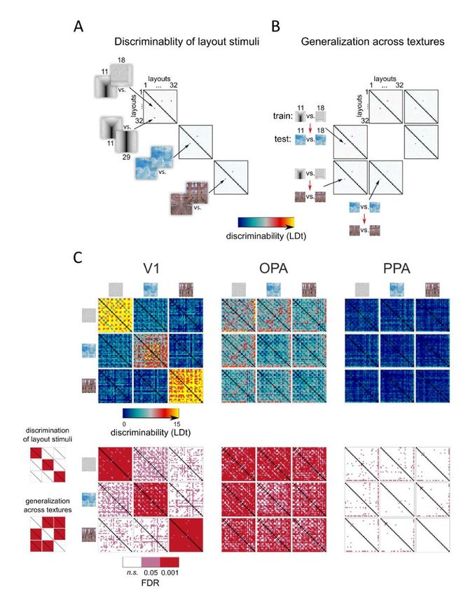
bioRxiv preprint first posted online Mar. 14, 2019; doi: http://dx.doi.org/10.1101/577064. The copyright holder for this preprint
 (which was not peer-reviewed) is the author/funder, who has granted bioRxiv a license to display the preprint in perpetuity.
                              It is made available under a CC-BY-NC-ND 4.0 International license.

       Author preprint, 13/3/2019

       SUMMARY

       Successful visual navigation requires a sense of the geometry of the local environment.

       How do our brains extract this information from retinal images? Here we visually

       presented scenes with all possible combinations of five scene-bounding elements (left,

       right and back wall, ceiling, floor) to human subjects during functional magnetic

       resonance imaging (fMRI) and magnetoencephalography (MEG). The fMRI response

       patterns in the scene-responsive occipital place area (OPA) reflected scene layout with

       invariance to changes in surface texture. This result contrasted sharply with the primary

       visual cortex (V1), which reflected low-level image features of the stimuli, and

       parahippocampal place area (PPA), which showed better texture than layout decoding.

       MEG indicated that the texture-invariant scene-layout representation is computed from

       visual input within ~100 ms, suggesting a rapid computational mechanism. Taken

       together, these results suggest that the cortical representation underlying our instant sense

       of the environmental geometry is located in OPA.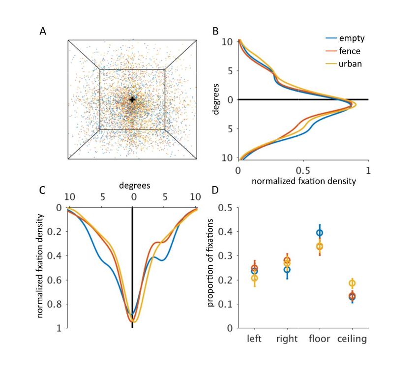
bioRxiv preprint first posted online Mar. 14, 2019; doi: http://dx.doi.org/10.1101/577064. The copyright holder for this preprint
 (which was not peer-reviewed) is the author/funder, who has granted bioRxiv a license to display the preprint in perpetuity.
                              It is made available under a CC-BY-NC-ND 4.0 International license.

       Author preprint, 13/3/2019

       INTRODUCTION

                Animals move around in their environments with grace and foresight, avoiding

       collisions with obstacles by charting viable paths based on their vision. This behaviour

       requires an animal’s visual system to provide its navigational circuits with information

       about the local environmental geometry. The human cortex contains visual areas that

       preferentially respond to visually presented scenes as compared to other stimuli, such as

       faces or objects. These areas include the parahippocampal place area (PPA; Epstein and

       Kanwisher, 1998) and the occipital place area (OPA; Grill-Spector, 2003; Dilks et al.,

       2013). PPA and OPA likely play a role in connecting visual perception with navigation,

       but their differential computational roles have not been fully established.

                Boundaries of open spaces, such as walls, constrain navigation and are therefore an

       essential aspect of the environmental geometry that our brains must represent (for a

       review, see Brunec et al., 2018). Even small children automatically use room geometry to

       reorient themselves (for a review, see Spelke et al., 2010). Recent neuroimaging studies

       suggest a role for human OPA in detecting navigationally important cues from visual

       scenes. A functional magnetic resonance imaging (fMRI) study demonstrated that OPA

       encodes possible paths in a visual scene (Bonner and Epstein, 2017), and if processing in

       the OPA is temporarily disrupted using transcranial magnetic stimulation (TMS), a

       person’s ability to use boundaries in a navigational task is impaired (Julian et al., 2016).

                Early fMRI studies already reported that the spatial layout, and not the presence of

       objects within the scene drives the scene-selective areas (Epstein and Kanwisher, 1998).

       Subsequent neuroimaging studies have made a distinction between open and closed

       sceneries (Harel et al., 2012; Kravitz et al., 2011; Park et al., 2011) and revealed the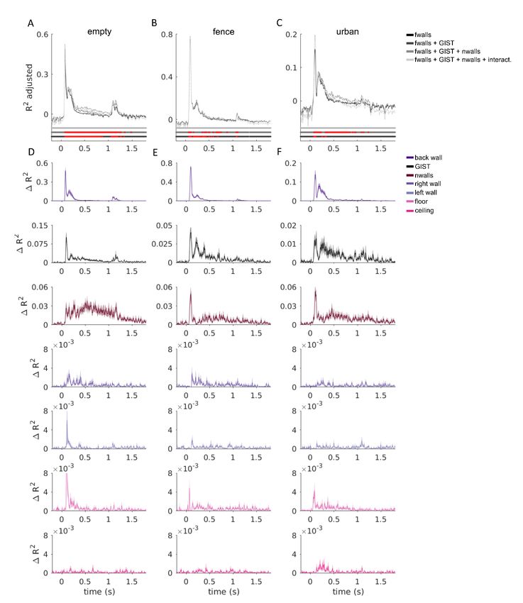
bioRxiv preprint first posted online Mar. 14, 2019; doi: http://dx.doi.org/10.1101/577064. The copyright holder for this preprint
 (which was not peer-reviewed) is the author/funder, who has granted bioRxiv a license to display the preprint in perpetuity.
                              It is made available under a CC-BY-NC-ND 4.0 International license.

       Author preprint, 13/3/2019

       relevance of the vertical height of boundaries (Ferrara and Park, 2016). However, exactly

       how scene-selective areas represent the geometry of the local environment has not been

       established.

                Here we ask how individual scene-bounding elements and their compositions are

       represented in scene-selective cortical areas. We test different brain regions for an explicit

       representation of the 3D geometry that is invariant to surface appearance. We created a

       novel set of synthetic scene stimuli, in which we systematically vary the spatial layout of

       the scene by switching on and off each of five spatial boundaries (three walls, floor, and

       ceiling; see Fig. 1). The resulting 25 = 32 layouts are rendered in three different styles of

       surface appearance (empty room, fences, urban space), yielding 96 scene stimuli. These

       stimuli were presented to 22 subjects, each of whom participated in both an fMRI and a

       magnetoencephalography (MEG) experiment. Whereas fMRI provides sufficiently high

       spatial resolution to resolve representations within a given brain region, MEG provides

       millisecond temporal resolution, enabling us to track the dynamics of cortical processing

       (Carlson et al., 2013; for a review, see Hari and Salmelin, 2012). We investigated to what

       extent OPA and PPA encode the scene layout in terms of the presence and absence of the

       scene-bounding elements, and how rapidly the respective representations emerge

       following stimulus onset.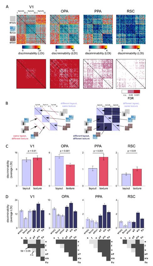
bioRxiv preprint first posted online Mar. 14, 2019; doi: http://dx.doi.org/10.1101/577064. The copyright holder for this preprint
 (which was not peer-reviewed) is the author/funder, who has granted bioRxiv a license to display the preprint in perpetuity.
                              It is made available under a CC-BY-NC-ND 4.0 International license.

       Author preprint, 13/3/2019

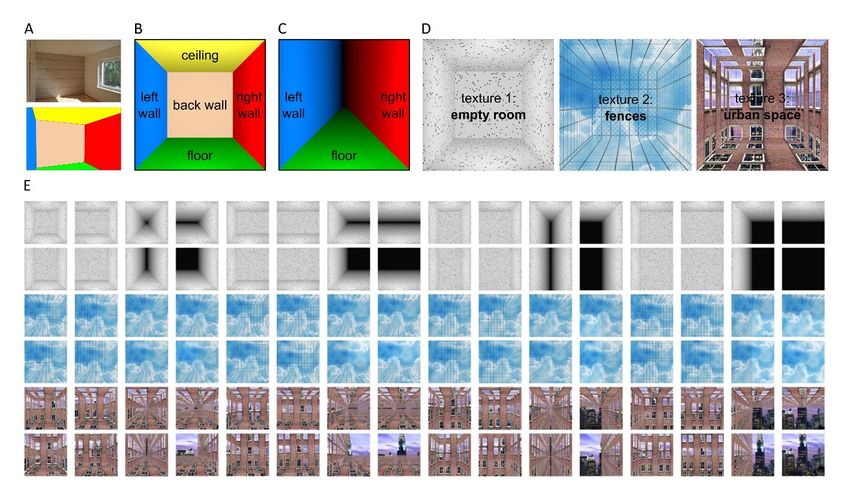
       Figure 1 | Stimuli to test the hypothesis that human scene-responsive cortical areas encode scene
       layout. A) The spatial layout of a room is captured by the fixed scene-bounding elements, such as the walls.
       B) We created a complete set of spatial layouts using 3D modelling software by switching on and off the five
       bounding elements: left wall, back wall, right wall, floor, and ceiling. C) For example, by switching off the back
       wall and the ceiling, we create a long, canyon-like environment. D) Textures and background images were
       added to the scenes to enable us to discern layout representations from low-level visual representations. E)
       The complete set of scenes included 32 different spatial layouts in 3 different textures, resulting in 96 scene
       stimuli.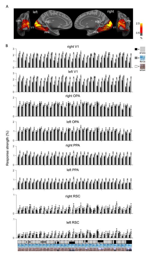
bioRxiv preprint first posted online Mar. 14, 2019; doi: http://dx.doi.org/10.1101/577064. The copyright holder for this preprint
 (which was not peer-reviewed) is the author/funder, who has granted bioRxiv a license to display the preprint in perpetuity.
                              It is made available under a CC-BY-NC-ND 4.0 International license.

       Author preprint, 13/3/2019

       RESULTS

       OPA discriminates layouts better than textures whereas the opposite is true for PPA

                We measured fMRI responses to the 96 different scene images (32 layouts in each of

       three different textures, Fig. 1E), while subjects fixated the stimuli centrally. Subjects

       were instructed to pay attention to the layout of the scene elements. Occasionally, the

       stimulus image was followed by an arrow pointing to one of five possible directions and

       the subject’s task was to tell with a button press whether the preceding layout had a

       bounding scene-element in that direction (e.g., an arrow pointing to the left would prompt

       the subject to report whether the left wall was present in the previous scene). Four regions

       of interest (ROIs) were defined based on criteria independent of the main experiment:

       primary visual cortex (V1) was defined on the basis of cortical sulci (Hinds et al., 2008),

       and OPA, PPA and retrosplenial cortex (RSC) were defined on the basis of functional

       localizer data using a different set of scenes, faces, objects, and textures as stimuli. Figure

       S1 shows the average responses separately for each stimulus in each ROI. In V1, the

       texture affected the response strength (empty < fence < urban), likely reflecting the

       amount of low-level image detail in the stimulus images. In OPA and PPA, the difference

       in response strength between the stimuli was smaller than in V1. In RSC, many of the

       stimuli did not evoke a measurable response, and hence, results for RSC are only shown in

       Supplementary Figures.

                First, we asked whether we can discriminate the fMRI response patterns evoked by

       the different scene stimuli. The discriminability of each pair of stimuli was evaluated by

       fitting a Fisher linear discriminant (Nili et al., 2014) to the response patterns from half of

       the fMRI data and by testing the performance on the response patterns from the other half

       of the fMRI data (split-half cross-validation). The analyses were done on individual data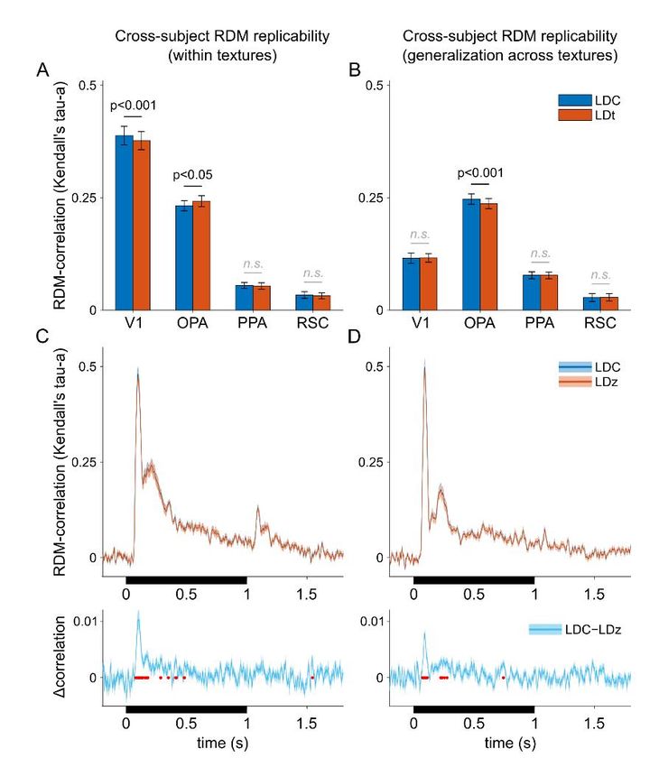
bioRxiv preprint first posted online Mar. 14, 2019; doi: http://dx.doi.org/10.1101/577064. The copyright holder for this preprint
 (which was not peer-reviewed) is the author/funder, who has granted bioRxiv a license to display the preprint in perpetuity.
                              It is made available under a CC-BY-NC-ND 4.0 International license.

       Author preprint, 13/3/2019

       and the results were pooled across the 22 subjects. First, we evaluated whether we can

       better discriminate the layout or the texture of a scene from the response patterns in

       different ROIs. Figure 2 shows the average linear-discriminant t (LDt) values for scenes

       that differ in layout (gray bars) and for scenes that differ in surface texture (black bars). In

       V1 and PPA, the LDt values were higher for texture than layout discrimination. Moreover,

       Figure S2 shows that in PPA, but not in V1, the scene discriminability was consistently

       higher when both the layout and the texture were different compared to scenes that only

       differed in their layout. As the texture defines the scene’s identity, these results suggest

       that PPA is involved in texture-based scene categorization rather than representing scene

       layout. In contrast to the results in PPA, in OPA the average discriminability was higher

       between scenes that differ in layout than in texture (Figure 2).

       Figure 2 | Layout vs. texture decoding. The average discriminability across all scene pairs that differ in the
       layout but are of the same texture (layout decoding; grey bars) and all scene pairs that have the same layout
       but differ in the texture (texture decoding; black bars) are shown separately for V1, OPA and PPA. In V1 and
       PPA, a change in the texture had on average a larger effect on the discriminability of the fMRI response-patterns
       than a change in the layout, whereas the opposite was true for OPA. The p-values are from two-tailed signed-
       rank tests across the 22 subjects; the error bars indicate standard errors of the mean (SEMs) across the
       subjects. See Figure S1 for average fMRI responses for all 96 individual stimuli for each region-of-interest, and
       Figure S2 for fMRI response-pattern discriminability separately for each stimulus pair.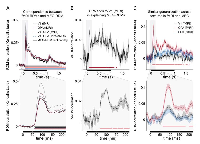
bioRxiv preprint first posted online Mar. 14, 2019; doi: http://dx.doi.org/10.1101/577064. The copyright holder for this preprint
 (which was not peer-reviewed) is the author/funder, who has granted bioRxiv a license to display the preprint in perpetuity.
                              It is made available under a CC-BY-NC-ND 4.0 International license.

       Author preprint, 13/3/2019

       Layout discrimination in OPA generalizes across surface-textures

                In order to test whether any of the regions contain a layout representation that is

       invariant to texture, we fit the linear discriminant to the response patterns for a pair of

       layouts in one texture and tested its performance with the same layouts in another texture.

       Successful cross-decoding across textures would suggest a scene-layout representation

       that is tolerant to a change in the surface-texture, and at the same time, rule out

       confounding effects of low-level image-feature differences on layout discrimination.

       Figure 3A-B shows a schematic illustration of the analysis. The distinctiveness of each

       layout pair is shown separately (diagonal matrices) as well as the ability of the

       discriminants to generalize to other surface-textures (off-diagonal matrices). These

       matrices will be referred to as representational dissimilarity matrices (RDMs).

                Figure 3C shows that in V1 the layouts evoked distinct response patterns, but the

       results did not generalize across textures. This result suggests that the pattern-

       discriminability in V1 was due to confounding low-level image feature differences

       between the same-texture spatial layouts instead of an explicit representation of layout. In

       OPA, on the contrary, the discriminants for stimulus pairs generalized across textures,

       suggesting that OPA encodes the layout of a visual scene invariantly to manipulations of

       surface texture. Finally, although PPA responded to the stimuli (Figure S1) and its average

       layout discriminability was above chance (Figure 2), its patterns did not enable reliable

       discrimination of most pairs of layouts (Figure 3C).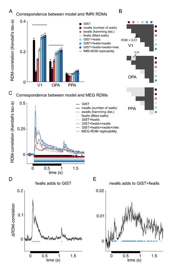
bioRxiv preprint first posted online Mar. 14, 2019; doi: http://dx.doi.org/10.1101/577064. The copyright holder for this preprint
 (which was not peer-reviewed) is the author/funder, who has granted bioRxiv a license to display the preprint in perpetuity.
                              It is made available under a CC-BY-NC-ND 4.0 International license.

       Author preprint, 13/3/2019

       Figure 3 | Discriminability of the fMRI response-patterns for each pair of layout stimuli in V1, OPA and
       PPA and the generalization of the result across textures. A) The discriminability of the layout stimuli from
       the fMRI response-patterns was evaluated for each pair of the 32 layouts, separately for the three textures. The
       Fisher linear discriminant was fitted to response-patterns obtained from training data (odd fMRI runs) and the
       performance was evaluated on independent testing data (even fMRI runs). The results are shown as linear
       discriminant t-values (LDt; Nili et al., 2014; Walther et al., 2016). The analyses were done on individual data
       and the results were pooled across subjects. B) The generalization of the layout discrimination across different
       surface textures was evaluated by fitting the Fisher linear discriminant to response-patterns corresponding to
       a pair of layouts in one texture and evaluating the performance on the response-patterns corresponding to the
       same layout pair in another texture. All combinations of texture pairs were evaluated. A high LDt-value suggests
       successful generalization of layout discrimination across surface textures, and hence a layout representation
       that is tolerant to a change in surface texture. C) The upper row shows the average LDt values for all pairs of
       stimuli. Along the diagonal, the three matrices reflect the distinctiveness of the response-patterns between each
       pair of layout stimuli in the same texture. The six off-diagonal matrices show generalization across textures
       (training between two layouts in one texture, testing on the same pair in another texture). The bottom row shows
       the expected false-discovery rates (FDR; n.s., not significant); the p-values were obtained using a two-sided
       signed-rank test across 22 subjects. In V1, the spatial layout stimuli elicited distinct response-patterns but the
       result did not generalize across textures. In OPA, most layouts evoked a distinct response-pattern and the
       results generalized across textures. In PPA, only few of the layouts evoked significantly different response
       patterns.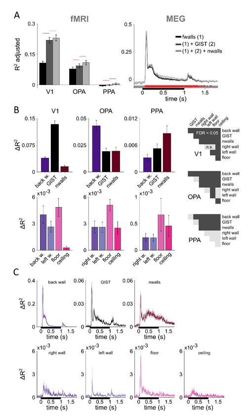
bioRxiv preprint first posted online Mar. 14, 2019; doi: http://dx.doi.org/10.1101/577064. The copyright holder for this preprint
 (which was not peer-reviewed) is the author/funder, who has granted bioRxiv a license to display the preprint in perpetuity.
                              It is made available under a CC-BY-NC-ND 4.0 International license.

       Author preprint, 13/3/2019

                Figure 4 shows the average LDt-RDMs and the corresponding false discovery rate

       matrices for V1, OPA and PPA, summarizing results from Figure 3. Corresponding

       multidimensional scaling (MDS) visualizations of the representational relationships are

       shown in Figure S3. The average RDMs and the MDS visualizations reveal that the

       presence of the back wall had a strong effect on the distinctiveness of the response

       patterns in V1, OPA, and PPA. In contrast to the other scene elements, the back wall

       covered a larger part of the visual field and was centred on the point of fixation. Given its

       larger retinal extent and the cortical magnification of the central region (Duncan and

       Boynton, 2003), the back wall had a much larger cortical representation than the other

       scene elements in early visual areas, especially in V1. In the scene-responsive regions, the

       added depth to the scenes by the removal of the back wall could also contribute to

       response-pattern discriminability. In OPA, we observe groupings that are consistent both

       in the within- and across-texture analysis (Figs. 4, S3). For example, pairs of scenes that

       only differed in the presence of the ceiling elicited similar response patterns (blue off-

       centre diagonal in the LDt-matrices), suggesting that the ceiling did not strongly

       contribute to the layout representation in OPA. Moreover, the number of the bounding

       elements present in the layout appears to have an effect on pattern distinctiveness (clusters

       in the MDS plots; Fig. S3).

                Although some layout-pairs could still be discriminated by the V1 response-patterns

       when the analysis was done across different textures (Fig. 4B), the overall decoding

       performance was significantly worse than when the analysis was done within the textures

       (Fig. 4A). In V1, but not in OPA, the representational geometry, as visualized using the

       MDS (Fig. S3), was also clearly different between the within-texture and cross-texture

       analyses. In PPA, the average discriminability of the layouts was low. OPA stands out
bioRxiv preprint first posted online Mar. 14, 2019; doi: http://dx.doi.org/10.1101/577064. The copyright holder for this preprint
(which was not peer-reviewed) is the author/funder, who has granted bioRxiv a license to display the preprint in perpetuity.
It is made available under a CC-BY-NC-ND 4.0 International license.
Author preprint, 13/3/2019
against V1 and PPA in that it discriminated spatial layouts of the same texture and the
result generalized across textures (middle panels in Fig. 4A and 4B). This finding is
consistent with a texture-invariant scene-layout representation in OPA.
Figure 4 | Representational geometry of scene layouts generalizes across textures in OPA. A) The
distinctiveness of the fMRI response-patterns for the spatial layouts are shown as captured by the LDt values.
The analyses done separately for the three textures were averaged (shown separately in Fig. 3). The lower row
shows the corresponding false discovery rates (two-tailed signed-rank test across 22 subjects). B) The
generalization performance of the discriminant across different textures was evaluated by fitting the linear
discriminant to a pair of spatial layouts in one texture and testing the discriminant on the same pair of layouts
in another texture. The analysis was done for each combination of textures and the results were averaged
(shown separately in Fig. 3). The lower row shows the corresponding false discovery rates. In OPA, the
representation shows texture-invariance. The multidimensional-scaling visualizations of the distinctiveness of
the response-patterns are shown in Figure S3.bioRxiv preprint first posted online Mar. 14, 2019; doi: http://dx.doi.org/10.1101/577064. The copyright holder for this preprint
(which was not peer-reviewed) is the author/funder, who has granted bioRxiv a license to display the preprint in perpetuity.
It is made available under a CC-BY-NC-ND 4.0 International license.
Author preprint, 13/3/2019
The OPA representation is reflected in early MEG responses
All subjects participated also in an MEG experiment to characterize the temporal
dynamics of scene-layout encoding. Similar to the fMRI experiments, the subjects fixated
the stimuli centrally and were instructed to pay attention to the layouts. Occasionally, the
stimulus image was followed by an arrow pointing to one of the five possible directions
and the subject’s task was to tell with a finger lift whether the preceding layout had a
scene-bounding element in that direction. Representational dissimilarity matrices were
constructed based on the cross-validated Mahalanobis distance between the evoked
responses of each pair of spatial layouts. For fMRI, the crossvalidated distance estimator
LDt was chosen based on previous results (Walther et al., 2016). For MEG, cross-
validated distance estimators are also recommended (Guggenmos et al., 2018), but the
effect of noise normalization is less well understood. We therefore used the crossvalidated
Mahalanobis distance (also termed linear discriminant contrast, LDC; Walther et al.,
2016), which omits the final noise normalization. Figure S4 shows a comparison of LDt
and LDC RDM reliability in our data. The MEG-RDMs were compared to the fMRI-
RDMs using Kendall’s tau-a rank correlation (Nili et al., 2014). The analyses were done
on individual data, separately for each texture. Representational dissimilarities were then
averaged across textures for each subject, and the significance testing treated subject as a
random effect.
Figure 5A shows that, as expected, both V1 and OPA fMRI-RDMs correlated with
the MEG-RDMs. To find out the unique contribution of the OPA to the correlation, MEG-
RDMs were fitted as a linear combination of the V1 and OPA fMRI-RDMs. OPA showed
a unique contribution to the MEG-RDM fit early after stimulus onset. The unique OPA
contribution becomes significant at 60 ms after stimulus onset (two-sided signed-rank testbioRxiv preprint first posted online Mar. 14, 2019; doi: http://dx.doi.org/10.1101/577064. The copyright holder for this preprint
(which was not peer-reviewed) is the author/funder, who has granted bioRxiv a license to display the preprint in perpetuity.
It is made available under a CC-BY-NC-ND 4.0 International license.
Author preprint, 13/3/2019
across subjects, multiple testing accounted for by controlling the false discovery rate at
.01) and peaks at about 100 ms (Fig. 5B). Importantly, only the OPA showed a significant
match between fMRI and MEG across-texture generalization of layout discriminants (Fig.
5C). In other words, MEG reflected the surface-texture invariant representation of the
spatial layouts similarly to the OPA fMRI-RDM, and the similarity emerged early in the
MEG data (significant at 65 ms, peaking at about 100 ms). These results suggest an early,
texture-invariant encoding of scene-layout in the OPA.
Figure 5 | Early correspondence between the representations in OPA (fMRI) and MEG. A) The Kendall
tau-a rank correlation between the MEG-RDMs and fMRI-RDMs are shown. The upper panel shows the full
time-course (stimulus-on period indicated by black bar) and the lower panel highlights the early time-window.
The black line shows the correlation between the MEG and V1-fMRI, and the dark red line shows the
correspondence between the MEG and OPA-fMRI. The correspondence between the MEG-RDMs and cross-
validated, fitted linear combinations of multiple fMRI-RDMs are also shown (light red line for V1 and OPA, blue
dashed line for V1, OPA and PPA). The analyses were done separately for each subject and for each texture,
and the results were averaged. Significant time points indicated with the thick lines (false-discovery rate, FDR,
of 0.01; p-values computed with two-tailed signed-rank test across the 22 subjects; FDR adjusted across time-
points). The grey line indicates the amount of replicable structure in the MEG-RDMs across subjects. Figure
S4 evaluates the effect of the distance estimator for the reliability of the RDMs. B) The OPA significantly adds
to V1 in explaining the MEG-RDMs already in the early time-window after stimulus onset. Shaded regions
indicate SEM across subjects, red line indicates false-discovery rate of 0.01 (two-tailed signed-rank test across
the 22 subjects; FDR across time points). C) Both MEG and fMRI -RDMs were also constructed based on how
well the layout discrimination results generalized across surface-textures (see also Figs. 3–4). Only OPA-fMRI,
not V1 or PPA, shows a significant correlation with MEG when the texture-generalized RDMs are compared
(red line indicates false discovery rate of 0.01 between OPA-fMRI-RDM and MEG-RDM; two-tailed signed-rank
test across the 22 subjects).bioRxiv preprint first posted online Mar. 14, 2019; doi: http://dx.doi.org/10.1101/577064. The copyright holder for this preprint
(which was not peer-reviewed) is the author/funder, who has granted bioRxiv a license to display the preprint in perpetuity.
It is made available under a CC-BY-NC-ND 4.0 International license.
Author preprint, 13/3/2019
Scene-bounding elements explain OPA representational geometry better than GIST
To characterize the geometries of the scene-layout representations, a set of models
(Fig. 6) was fitted to the fMRI- and MEG-RDMs. We aimed to model both the
contribution of the low-level image features and the presence of the scene-bounding
elements. The GIST (Oliva and Torralba, 2001) model was included to capture low-level
image feature differences between the scene stimuli. Separate GIST RDMs were
constructed for each texture. The first scene-layout-based RDM model consisted of the
Hamming distance between the binary vectors, indicating which scene-bounding elements
were present and absent. For each pair of scenes, the Hamming distance is the number of
discrepant scene-bounding elements. The Hamming distance assigns equal importance to
all elements: vertical walls, floor, and ceiling. Hence, we name this model “ewalls” to
stand for equally weighted walls (see top row in Fig. 6). In order to model the possibility
that the brain representation does not weight all scene-bounding elements equally, we
included a separate RDM component for each of the five scene-bounding elements and
modelled the RDM as a fitted linear combination of the components (model “fwalls”, for
fitted walls; middle row in Fig. 6). In addition, the number of walls present in a scene was
included (model “nwalls”, for number of walls; top row in Fig. 6), predicting similar
response patterns for two layouts with a similar number of walls. This model can be
interpreted as reflecting the size of the space depicted in the scene (ranging from open to
closed). For possible interaction effects between specific scene-elements (e.g., the
presence of both the floor and the left wall forming an edge), interaction models were also
constructed (two bottom rows in Fig. 6). The models were fitted using non-negative least
squares (Khaligh-Razavi and Kriegeskorte, 2014) and tested by crossvalidation across
subjects.bioRxiv preprint first posted online Mar. 14, 2019; doi: http://dx.doi.org/10.1101/577064. The copyright holder for this preprint
(which was not peer-reviewed) is the author/funder, who has granted bioRxiv a license to display the preprint in perpetuity.
It is made available under a CC-BY-NC-ND 4.0 International license.
Author preprint, 13/3/2019
Figure 6 | The representational geometries were modelled as linear combinations of representational
components. The first three model-RDMs capture the GIST features (Oliva and Torralba, 2001) of the stimuli
(low-level image feature similarity), shown separately for the three different textures. The next model predicts
the responses for a scene-layout-based representation with equal contribution of all walls, calculated as the
hamming distance between the layouts (percentage of same boundaries present in a pair of scenes; predicting
a similar response to two scenes with same boundaries and distinct response for a pair of scenes with different
boundaries). The last model on the top row is constructed based on the number of scene-bounding elements
present in each scene (similar response to a pair of scenes with the same number of scene-elements present
in the scene), roughly reflecting the size of the space. The middle row shows the five model-RDMs capturing
separately the presence of each of the five scene-bounding elements in the spatial layouts. The last ten model-
RDMs reflect the interactions between the walls.bioRxiv preprint first posted online Mar. 14, 2019; doi: http://dx.doi.org/10.1101/577064. The copyright holder for this preprint
(which was not peer-reviewed) is the author/funder, who has granted bioRxiv a license to display the preprint in perpetuity.
It is made available under a CC-BY-NC-ND 4.0 International license.
Author preprint, 13/3/2019
The GIST model explained the V1 RDM (fMRI) better than any of the scene-layout
models (nwalls, ewalls, fwalls; Fig. 7A–B). For OPA, results were strikingly different.
The GIST model was still better than the number of walls (nwalls, reflecting the degree of
openness) at explaining the OPA RDM (Fig. 7A–B) but there was no significant
difference between the GIST model and the scene-layout model with equal contribution of
each scene-bounding element (ewalls, Fig. 7A–B). Moreover, the fitted combination of
scene-bounding elements model (fwalls) captured the representation significantly better
than the GIST model (Fig. 7A–B). Adding the GIST component and the wall-specific
RDM components in a fitted model did not increase explained variance in OPA (it did in
V1). Explained variance in OPA was increased by adding the number-of-walls
component, suggesting that scene openness is reflected the representation. Finally, adding
components for the interactions between the scene-bounding elements increased the
explained variance slightly in both V1 and OPA. In PPA, the best predictions were
obtained by combining all the components (GIST, walls with fitted weights, number of
walls). In contrast to V1 and OPA, however, adding the interaction components did not
significantly improve predictions for PPA.bioRxiv preprint first posted online Mar. 14, 2019; doi: http://dx.doi.org/10.1101/577064. The copyright holder for this preprint
(which was not peer-reviewed) is the author/funder, who has granted bioRxiv a license to display the preprint in perpetuity.
It is made available under a CC-BY-NC-ND 4.0 International license.
Author preprint, 13/3/2019
Figure 7 | The contributions of low-level image differences and true scene-layout based representations
in the fMRI- and MEG-RDMs. A) The mean Kendall’s tau-a correlation between the models and fMRI-RDMs
are shown separately for V1, OPA and PPA. In V1, there is only a small improvement in the correlations when
the GIST model is complemented with other models. In OPA, the fitted combination of scene-bounding
elements model (fwalls) alone already explain the representation better than the GIST model. The grey lines
indicate the amount of replicable structure in the fMRI-RDMs across subjects. The error bars indicate standard
errors of the mean (SEMs) across the subjects. B) Pairwise comparisons between the models, shown
separately for V1, OPA and PPA. The color-codes and order of the models is the same as in (A). Dark grey
colour indicates significant difference between the models (two-tailed signed-rank tests across the 22 subjects,
multiple testing accounted for by controlling the false discovery rate at .01), light grey indicates non-significance.
C) The time-courses of the model-RDM fits to the MEG-RDMs are shown. The colours are the same as in (A).
The grey line indicates the amount of replicable structure in the MEG-RDMs across subjects. The thick lines
indicate significant correlations (false discovery rate of 0.01 based on two-tailed signed-rank tests across the
22 subjects). The black rectangle shows the timing of the stimulus. D) The mean increase in the Kendall’s tau
a rank correlation is shown when the fitted wall-RDMs were included in the fitting compared to having only the
GIST model. Time-points with significant increase are indicated with the blue lines (false discovery rate 0.01;
two-tailed signed-rank test across subjects). E) Including the RDM based on the number of walls present in the
scenes further increased the model fit, especially at the later timepoints (blue lines indicate false discovery rate
0.01; two-tailed signed-rank test across subjects).bioRxiv preprint first posted online Mar. 14, 2019; doi: http://dx.doi.org/10.1101/577064. The copyright holder for this preprint
(which was not peer-reviewed) is the author/funder, who has granted bioRxiv a license to display the preprint in perpetuity.
It is made available under a CC-BY-NC-ND 4.0 International license.
Author preprint, 13/3/2019
Figure 7C shows the model crossvalidation results for the MEG RDMs, illustrating
the dynamics of how the different models (Fig. 6) captured the representations. As
expected, the GIST model captured the early representation (black line). However,
including the scene-bounding elements improved the fit early. Figure 7D shows the unique
contribution that scene-bounding elements added to the GIST model, peaking at about 100
ms after stimulus onset. Similar to the fMRI modelling, the contribution of each of the
scene-bounding elements was modelled separately and the result was crossvalidated across
subjects. Moreover, consistent with the fMRI results for OPA and PPA, the number of
walls present in the scene also significantly contributed to the MEG-RDMs, especially at
the later timepoints (Fig. 7E).
To further evaluate the contribution of each representational component, Figure 8
shows how much is gained in total explained variance by each of the model components.
The analysis was done by leaving out each model component in turn and evaluating the
proportion of variance explained between the full model and the reduced model. The
interactions (two bottom rows in Fig. 6) were excluded from the full model as they did not
significantly increase the adjusted explained variance in fMRI or MEG data (see Figs. S5–
S6). The GIST model dominates the explained variance in V1. In both V1 and OPA
(fMRI), the contribution of the back wall was stronger compared to the other walls, likely
reflecting its larger visual field extent, and in OPA possibly also reflecting the added depth
to the scenes by the removal of the back wall. In OPA, the floor had a significantly larger
contribution than the right wall, the left wall, and the ceiling (two-sided signed-rank test
across subjects, multiple testing accounted for by controlling the false discovery rate at
.05). In the MEG results, corresponding results were found with the GIST model
dominating the gain in the explained variance, but also a pronounced representation of thebioRxiv preprint first posted online Mar. 14, 2019; doi: http://dx.doi.org/10.1101/577064. The copyright holder for this preprint
(which was not peer-reviewed) is the author/funder, who has granted bioRxiv a license to display the preprint in perpetuity.
It is made available under a CC-BY-NC-ND 4.0 International license.
Author preprint, 13/3/2019
floor compared to right and left wall and the ceiling (bottom row in Fig. 8C), consistent
with the results found in OPA (fMRI).
Figure 8 | The unique variance explained by each model component. A) The explained variance (R2
adjusted) of the fitted joint models containing components for the five scene-bounding elements (black
bars/line), components for the five scene-bounding elements and the GIST (dark grey bars/line), and
components for the five scene-bounding elements, the GIST, and the number of walls (light grey bars/line). The
red lines indicate a significant improvement compared to a model with fewer components (one-tailed signed-
rank tests across the 22 subjects, multiple testing within a region-of-interest or across time-points accounted
for by controlling the false discovery rate at .05). See Figures S5–6 for the results for each texture separately
and including also the component models for interactions between walls (overall no further improvement in the
adjusted explained variance). B) The gain in the variance explained by each of the model components was
calculated by comparing the explained variance between the full model (light grey in A) with a model where this
one component was left out from the joint fit. Each model component was left out in turn, and the results are
shown separately for B) V1, OPA and PPA (fMRI) and C) MEG data. Error bars (fMRI) and shaded regions
(MEG) are standard errors of the mean across subjects. In different regions-of-interest (fMRI), the different
model components made different contributions to the representation; see the half-matrices for results from
significance testing (two-tailed signed-rank tests across the 22 subjects, multiple testing within a region-of-
interest accounted for by controlling the false discovery rate at .05). The pronounced contribution of the floor to
the scene representations (fMRI-OPA and MEG) is consistent with the behavioural results shown in Figure S7.bioRxiv preprint first posted online Mar. 14, 2019; doi: http://dx.doi.org/10.1101/577064. The copyright holder for this preprint
(which was not peer-reviewed) is the author/funder, who has granted bioRxiv a license to display the preprint in perpetuity.
It is made available under a CC-BY-NC-ND 4.0 International license.
Author preprint, 13/3/2019
Fixations during free viewing favour the floor over the ceiling
Before the neuroimaging experiments, all 22 subjects participated in a behavioural
experiment to familiarize themselves with the stimuli. The subjects were shown the 96
stimulus images (Fig. 1E) once in a random order. We tracked their eye gaze when they
freely explored the scenes. The presentation time was short (1 second) and the subjects
were asked to always bring their gaze back to the central fixation cross between the
stimuli. Without any specific instructions on where or what to look at in the images,
subjects made more saccades to the lower than upper visual field, and more specifically, to
the floor than to the ceiling (Fig. S7; FDR = 0.0035; 0.0077; 0.003 for each texture
separately; two-tailed signed-rank test across 22 subjects, FDR across the combinations of
wall pairs). This result suggests that attention is automatically directed to the lower parts
of a scene, where the navigationally crucial geometry of the ground appears. The
prioritized processing of the ground geometry is consistent with our neuroimaging results,
where subjects maintained central fixation, but OPA exhibited a more prominent
representation of the floor (compared to the ceiling and the left and right walls; Fig. 8B).bioRxiv preprint first posted online Mar. 14, 2019; doi: http://dx.doi.org/10.1101/577064. The copyright holder for this preprint
(which was not peer-reviewed) is the author/funder, who has granted bioRxiv a license to display the preprint in perpetuity.
It is made available under a CC-BY-NC-ND 4.0 International license.
Author preprint, 13/3/2019
DISCUSSION
Visual navigation requires that the human brain represent the geometry of the
environment, and especially the physical bounds of navigable space (Spelke and Lee,
2012). We refer to the stable geometric shape of the space bounded by walls, floor and the
ceiling as the layout of the scene. Our results suggest that the scene-bounding elements are
extracted from the visual input by the scene-responsive cortical area OPA. Specifically,
using fMRI, we found that OPA encodes scene layout in a format that supports linear
readout of the presence or absence of bounding elements with invariance to manipulations
of surface texture. The representation in V1 was better captured by a model of low-level
image features of the scene stimuli than the presence of the walls, whereas in OPA, the
presence of the walls captured the representation better. PPA did not reliably distinguish
the scene layouts in its fMRI response patterns, and overall, PPA showed better decoding
performance for scene texture than layout, which was opposite to the results found in
OPA. Texture is closely related to the category of the scene (e.g. indoor versus outdoor,
urban versus natural). Our results hence support the view that OPA is involved in
extracting the spatial structure of the local environment, whereas PPA has a role in scene
recognition (Julian et al., 2018). We complemented the fMRI results with high-temporal-
resolution MEG data. Scene-layout representations with similar invariance to surface
texture as found in OPA with fMRI emerged rapidly after stimulus onset in the MEG
responses (peaking at ~100 ms). The rapid emergence of an explicit encoding of scene
layout in human OPA is consistent with recent modeling work suggesting that a layout
representation can be efficiently computed by a feedforward mechanism (Bonner and
Epstein, 2018).bioRxiv preprint first posted online Mar. 14, 2019; doi: http://dx.doi.org/10.1101/577064. The copyright holder for this preprint
(which was not peer-reviewed) is the author/funder, who has granted bioRxiv a license to display the preprint in perpetuity.
It is made available under a CC-BY-NC-ND 4.0 International license.
Author preprint, 13/3/2019
Our stimulus set systematically varied the presence of five scene-bounding elements
(three walls, floor, and ceiling) for a total of 25 = 32 environmental geometries, each of
which was rendered in three different surface textures. This systematic set enabled us to
investigate the relative contribution of each of the five scene-bounding elements to the
representations. The back wall covered a much larger, and more central, part of the visual
field and thus mapped onto a larger patch of cortical surface in V1 (Duncan and Boynton,
2003) than other scene-bounding elements. The back wall was also prominently
represented in downstream scene-responsive regions, which might reflect both its early
visual representation and its navigational relevance in limiting forward movement. The
removal of the back wall also adds depth to the scenes but the current stimuli were not
optimised for fully disentangling the contribution of perceived depth from confounding
low-level image features. Lescroart et al. (2015) have previously looked at the relationship
between Fourier power and subjective distance in natural scenes. They conclude that these
models provide similar predictions of brain activity in OPA and PPA when the responses
to natural scenes are analysed using voxel-wise encoding models and suggest that some
previous fMRI studies reporting representations of distance in scene-responsive cortical
areas might be affected by this confound. More recently, Lescroart et al. (2019) used
computer-generated stimuli similar to ours to model the relative contributions of low-level
features and 3D structure on the voxel responses to scenes across the visual cortex. They
report that individual voxels in scene-responsive areas represent combinations of
orientations and distances of surfaces and, overall, that distance and openness are
represented in OPA, PPA and RSC. Our results complement their results by showing a
dissociation between the representations in OPA and PPA, with only OPA exhibiting abioRxiv preprint first posted online Mar. 14, 2019; doi: http://dx.doi.org/10.1101/577064. The copyright holder for this preprint
(which was not peer-reviewed) is the author/funder, who has granted bioRxiv a license to display the preprint in perpetuity.
It is made available under a CC-BY-NC-ND 4.0 International license.
Author preprint, 13/3/2019
texture-invariant representation of scene layout, and by revealing the rapid emergence of
this representation in the MEG responses.
The right and left wall, the ceiling and the floor all covered equal-sized regions in
the visual field in our stimulus set, and hence, enabled comparisons of their relative
contributions to the representations. The ceiling and floor differed from the left and right
walls in terms of their prominence in the cortical representations. In V1, the ceiling was
more weakly represented than the other scene elements, which is likely explained by the
asymmetry between the upper and lower visual field representations in V1 (Henriksson et
al., 2012; Liu et al., 2006). Overall, however, low-level image feature differences between
the stimulus images better captured the representation in V1 than any scene-layout-based
model. OPA exhibited a more prominent representation of the floor than of the left and
right walls and the ceiling. One interpretation of this result is that the ground ahead of us
has a special status in the OPA representation because it supports our movement in the
environment. A special status for the ground is also supported by the eye-gaze data,
collected before the neuroimaging experiments, which showed that subjects paid more
attention to the floor than to the ceiling when viewing the novel scenes.
Consistent with our findings, previous studies have shown that OPA (also named
transverse occipital sulcus, TOS) has lower- and peripheral-visual-field biases (Silson et
al., 2015; Levy et al., 2004, 2001). An important question for future work is to what extent
OPA represents the geometry of the ground ahead or more general features of the lower
visual field. The OPA representation most likely reflects the natural regularities of the
environment and the functional importance of different features. During normal navigation
gaze is typically directed ahead, and hence, the floor is perceived in the lower peripheralbioRxiv preprint first posted online Mar. 14, 2019; doi: http://dx.doi.org/10.1101/577064. The copyright holder for this preprint
(which was not peer-reviewed) is the author/funder, who has granted bioRxiv a license to display the preprint in perpetuity.
It is made available under a CC-BY-NC-ND 4.0 International license.
Author preprint, 13/3/2019
visual field from where information is sampled to avoid obstacles and to adjust steps
according to the terrain (Marigold and Patla, 2008; Turano et al., 2001). We have
previously proposed that the occipital face area (OFA) might develop from a perifoveal
retinotopic protomap into a map of face-feature detectors arranged on the cortical sheet in
the topology of a face (the “faciotopy” hypothesis; Henriksson et al., 2015). The
neighboring scene-responsive cortex has a peripheral visual-field bias (Levy et al., 2001,
2004) and might similarly develop from a retinotopic protomap into a representation of
scene layout, with extended representations of the behaviourally most relevant features.
A limitation of the current study is the use 2D renderings of the scenes instead of 3D
stimulus presentation. The literature on navigation has used virtual reality (VR) much
more rigorously (for an example, see Hartley et al., 2003) than studies on visual
perception, although scene perception studies would also benefit from 3D stimuli and
interaction with the scenes. Challenges with more complex stimuli are stimulus control
and how to reliably analyze and interpret the data. In the future, combining MEG with VR
might allow novel experiments aimed at understanding the smooth interplay between
visual perception and navigation during natural behavior. Furthermore, the scenes that we
used as the stimuli likely varied in how plausible they are in the context of environments
that we naturally encounter. We wanted to use a full stimulus set where the presence
(absence) of each wall was equally possible. Future studies could reveal how cortical
representations differ between scene layouts that are typically encountered and layouts
that are improbable to encounter. Moreover, the use of a more restricted set of layouts
with a wider set of textures could further help tease apart perceptual differences that in our
stimuli might co-vary with the change in the layout, for example, related to perceived
distance in a scene.bioRxiv preprint first posted online Mar. 14, 2019; doi: http://dx.doi.org/10.1101/577064. The copyright holder for this preprint
(which was not peer-reviewed) is the author/funder, who has granted bioRxiv a license to display the preprint in perpetuity.
It is made available under a CC-BY-NC-ND 4.0 International license.
Author preprint, 13/3/2019
The functional roles of scene-responsive cortical visual areas OPA, PPA and
retrosplenial cortex (RSC; Maguire, 2001) are often discussed in the context of navigation,
but the interplay between visual perception and navigation is not yet fully understood.
Navigation is thought to rely on a cognitive-map-like representation of the environment in
the hippocampus that might be anchored to the visually perceived environment with the
help of landmarks by the RSC (Epstein et al., 2017). Though PPA was originally linked to
the perception of the spatial layout of the environment (Epstein and Kanwisher, 1998),
cumulative evidence suggests that PPA is primarily involved in recognizing the scene
category (e.g. kitchen versus woods) and scene identity (e.g. our kitchen versus someone
else’s) using a combination of geometry and texture cues, whereas OPA is involved in the
analysis of the local scene elements (Bonner and Epstein, 2017; Julian et al., 2018; Kamps
et al., 2016; Lowe et al., 2017). Scenes that we recognize as distinct places might have
identical layout and it is the textures and object ensembles that provide the crucial cues to
where we are. Scene perception mostly happens in the peripheral visual field, which is
limited by visual acuity but especially by visual crowding (Rosenholtz, 2016). PPA may
extract the identity of the scene by encoding the summary statistics of object ensembles
present in the scene (Cant and Xu, 2012). Overall, our results on the better texture than
layout encoding in the PPA are in agreement with previous studies showing texture
information in human PPA (Park and Park, 2017) and in the putative PPA homologue in
macaques (Kornblith et al., 2013).
In conclusion, our study shows a striking distinction between PPA, which did not
enable reliable decoding of scene layout, and OPA, whose activity patterns reflected the
presence or absence of each of the five spatial constraints with invariance to surface
texture. These results support the view that the OPA extracts information about a scene’sbioRxiv preprint first posted online Mar. 14, 2019; doi: http://dx.doi.org/10.1101/577064. The copyright holder for this preprint
(which was not peer-reviewed) is the author/funder, who has granted bioRxiv a license to display the preprint in perpetuity.
It is made available under a CC-BY-NC-ND 4.0 International license.
Author preprint, 13/3/2019
spatial structure, whereas PPA is involved in recognizing the scene context (Julian et al.,
2018). Our analyses reveal the emergence, within 100 ms of stimulus onset, of a detailed
encoding of scene layout in OPA, suggesting that this cortical region supports our rapid
visual sense of the geometry of our environment.
Acknowledgements: This work was supported by the Academy of Finland Postdoctoral
Researcher Grant (278957) to LH, a British Academy Postdoctoral Fellowship
(PS140117) to MM, and a European Research Council Starting Grant (ERC-2010-StG
261352) to NK. We thank ANI staff (especially Marita Kattelus, Mia Illman and Veli-
Matti Saarinen) for assistance with the measurements. We acknowledge the computational
resources provided by the Aalto Science-IT project.
Author Contributions: Conceptualization, L.H., M.M., N.K.; Methodology, L.H., M.M.,
N.K.; Software, L.H., N.K.; Validation, L.H.; Formal Analysis, L.H.; Investigation, L.H.;
Resources, L.H.; Data Curation, L.H.; Writing – Original Draft Preparation, L.H., M.M.,
N.K.; Writing – Review & Editing, L.H., M.M., N.K.; Visualization, L.H.; Supervision,
L.H., N.K.; Project Administration, L.H.; Funding Acquisition, L.H.
Declaration of interests: The authors declare no competing interests.bioRxiv preprint first posted online Mar. 14, 2019; doi: http://dx.doi.org/10.1101/577064. The copyright holder for this preprint
(which was not peer-reviewed) is the author/funder, who has granted bioRxiv a license to display the preprint in perpetuity.
It is made available under a CC-BY-NC-ND 4.0 International license.
Author preprint, 13/3/2019
REFERENCES
Bonner, M.F., and Epstein, R.A. (2017). Coding of navigational affordances in the human
visual system. Proc. Natl. Acad. Sci. U. S. A. 114, 4793–4798.
Bonner, M.F., and Epstein, R.A. (2018). Computational mechanisms underlying cortical
responses to the affordance properties of visual scenes. PLoS Comput. Biol. 14, e1006111.
Brunec, I.K., Moscovitch, M., and Barense, M.D. (2018). Boundaries Shape Cognitive
Representations of Spaces and Events. Trends Cogn. Sci.
Cant, J.S., and Xu, Y. (2012). Object ensemble processing in human anterior-medial
ventral visual cortex. J. Neurosci. 32, 7685–7700.
Carlson, T., Tovar, D.A., Alink, A., and Kriegeskorte, N. (2013). Representational
dynamics of object vision: the first 1000 ms. J. Vis. 13, 1–1.
Dale, A.M., Fischl, B., and Sereno, M.I. (1999). Cortical surface-based analysis: I.
Segmentation and surface reconstruction. Neuroimage 9, 179–194.
Dilks, D.D., Julian, J.B., Paunov, A.M., and Kanwisher, N. (2013). The occipital place
area is causally and selectively involved in scene perception. J. Neurosci. 33, 1331–1336.
Duncan, R.O., and Boynton, G.M. (2003). Cortical magnification within human primary
visual cortex correlates with acuity thresholds. Neuron 38, 659–671.
Epstein, R., and Kanwisher, N. (1998). A cortical representation of the local visual
environment. Nature 392, 598–601.
Epstein, R.A., Patai, E.Z., Julian, J.B., and Spiers, H.J. (2017). The cognitive map in
humans: spatial navigation and beyond. Nat. Neurosci. 20, 1504.
Ferrara, K., and Park, S. (2016). Neural representation of scene boundaries.
Neuropsychologia 89, 180–190.
Gramfort, A., Luessi, M., Larson, E., Engemann, D.A., Strohmeier, D., Brodbeck, C.,
Parkkonen, L., and Hämäläinen, M.S. (2014). MNE software for processing MEG and
EEG data. Neuroimage 86, 446–460.
Grill-Spector, K. (2003). The neural basis of object perception. Curr. Opin. Neurobiol. 13,
159–166.
Guggenmos, M., Sterzer, P., and Cichy, R.M. (2018). Multivariate pattern analysis for
MEG: A comparison of dissimilarity measures. NeuroImage 173, 434–447.
Harel, A., Kravitz, D.J., and Baker, C.I. (2012). Deconstructing visual scenes in cortex:
gradients of object and spatial layout information. Cereb. Cortex 23, 947–957.
Hari, R., and Salmelin, R. (2012). Magnetoencephalography: from SQUIDs to
neuroscience: Neuroimage 20th anniversary special edition. Neuroimage 61, 386–396.bioRxiv preprint first posted online Mar. 14, 2019; doi: http://dx.doi.org/10.1101/577064. The copyright holder for this preprint
(which was not peer-reviewed) is the author/funder, who has granted bioRxiv a license to display the preprint in perpetuity.
It is made available under a CC-BY-NC-ND 4.0 International license.
Author preprint, 13/3/2019
Hartley, T., Maguire, E.A., Spiers, H.J., and Burgess, N. (2003). The well-worn route and
the path less traveled: distinct neural bases of route following and wayfinding in humans.
Neuron 37, 877–888.
Henriksson, L., Karvonen, J., Salminen-Vaparanta, N., Railo, H., and Vanni, S. (2012).
Retinotopic maps, spatial tuning, and locations of human visual areas in surface
coordinates characterized with multifocal and blocked FMRI designs. PloS One 7,
e36859.
Henriksson, L., Mur, M., and Kriegeskorte, N. (2015). Faciotopy—a face-feature map
with face-like topology in the human occipital face area. Cortex 72, 156–167.
Hinds, O.P., Rajendran, N., Polimeni, J.R., Augustinack, J.C., Wiggins, G., Wald, L.L.,
Rosas, H.D., Potthast, A., Schwartz, E.L., and Fischl, B. (2008). Accurate prediction of
V1 location from cortical folds in a surface coordinate system. Neuroimage 39, 1585–
1599.
Julian, J.B., Ryan, J., Hamilton, R.H., and Epstein, R.A. (2016). The occipital place area is
causally involved in representing environmental boundaries during navigation. Curr. Biol.
26, 1104–1109.
Julian, J.B., Keinath, A.T., Marchette, S.A., and Epstein, R.A. (2018). The neurocognitive
basis of spatial reorientation. Curr. Biol. 28, R1059–R1073.
Kamps, F.S., Julian, J.B., Kubilius, J., Kanwisher, N., and Dilks, D.D. (2016). The
occipital place area represents the local elements of scenes. NeuroImage 132, 417–424.
Khaligh-Razavi, S.-M., and Kriegeskorte, N. (2014). Deep supervised, but not
unsupervised, models may explain IT cortical representation. PLoS Comput Biol 10,
e1003915.
Kornblith, S., Cheng, X., Ohayon, S., and Tsao, D.Y. (2013). A network for scene
processing in the macaque temporal lobe. Neuron 79, 766–781.
Kravitz, D.J., Peng, C.S., and Baker, C.I. (2011). Real-world scene representations in
high-level visual cortex: it’s the spaces more than the places. J. Neurosci. 31, 7322–7333.
Kriegeskorte, N., and Kievit, R.A. (2013). Representational geometry: integrating
cognition, computation, and the brain. Trends Cogn. Sci. 17, 401–412.
Kriegeskorte, N., Formisano, E., Sorger, B., and Goebel, R. (2007). Individual faces elicit
distinct response patterns in human anterior temporal cortex. Proc. Natl. Acad. Sci. 104,
20600–20605.
Kriegeskorte, N., Mur, M., and Bandettini, P.A. (2008). Representational similarity
analysis-connecting the branches of systems neuroscience. Front. Syst. Neurosci. 2, 4.
Lescroart, M.D., and Gallant, J.L. (2019). Human scene-selective areas represent 3D
configurations of surfaces. Neuron 101, 178-192. e7.You can also read


