Quantitative estimation of soil salinity by means of different modeling methods and visible-near infrared (VIS-NIR) spectroscopy, Ebinur Lake ...
←
→
Page content transcription
If your browser does not render page correctly, please read the page content below

Quantitative estimation of soil salinity by
                               means of different modeling methods
                               and visible-near infrared (VIS–NIR)
                               spectroscopy, Ebinur Lake Wetland,
                               Northwest China
                               Jingzhe Wang, Jianli Ding, Aerzuna Abulimiti and Lianghong Cai
                               College of Resources and Environment Science, Xinjiang University, Urumqi, Xinjiang, China
                               Key Laboratory of Smart City and Environment Modelling of Higher Education Institute,
                               Xinjiang University, Urumqi, Xinjiang, China
                               Key Laboratory of Oasis Ecology, Xinjiang University, Urumqi, Xinjiang, China

                                   ABSTRACT
                                   Soil salinization is one of the most common forms of land degradation. The detection
                                   and assessment of soil salinity is critical for the prevention of environmental dete-
                                   rioration especially in arid and semi-arid areas. This study introduced the fractional
                                   derivative in the pretreatment of visible and near infrared (VIS–NIR) spectroscopy.
                                   The soil samples (n = 400) collected from the Ebinur Lake Wetland, Xinjiang Uyghur
                                   Autonomous Region (XUAR), China, were used as the dataset. After measuring the
                                   spectral reflectance and salinity in the laboratory, the raw spectral reflectance was
                                   preprocessed by means of the absorbance and the fractional derivative order in the
                                   range of 0.0–2.0 order with an interval of 0.1. Two different modeling methods, namely,
                                   partial least squares regression (PLSR) and random forest (RF) with preprocessed
                                   reflectance were used for quantifying soil salinity. The results showed that more spectral
                                   characteristics were refined for the spectrum reflectance treated via fractional derivative.
                                   The validation accuracies showed that RF models performed better than those of PLSR.
                                   The most effective model was established based on RF with the 1.5 order derivative
Submitted 12 February 2018         of absorbance with the optimal values of R2 (0.93), RMSE (4.57 dS m−1 ), and RPD
Accepted 14 April 2018             (2.78 ≥ 2.50). The developed RF model was stable and accurate in the application
Published 3 May 2018               of spectral reflectance for determining the soil salinity of the Ebinur Lake wetland.
Corresponding author               The pretreatment of fractional derivative could be useful for monitoring multiple soil
Jianli Ding, ding_jl@163.com       parameters with higher accuracy, which could effectively help to analyze the soil salinity.
Academic editor
Danlin Yu
                               Subjects Soil Science, Data Mining and Machine Learning, Natural Resource Management,
Additional Information and
Declarations can be found on   Environmental Impacts, Spatial and Geographic Information Science
page 19                        Keywords Ebinur Lake, RF, VIS–NIR, PLSR, Soil salinity, Machine learning, Wetland

DOI 10.7717/peerj.4703

    Copyright                  INTRODUCTION
2018 Wang et al.
                               Soil salinization is one of the most common forms and drivers of land degrada-
Distributed under              tion, and entails significant environmental, social, and economic consequences,
Creative Commons CC-BY 4.0
                               especially in arid and semi-arid areas (Akramkhanov et al., 2011; Ding & Yu, 2014;
OPEN ACCESS                    Nawar, Buddenbaum & Hill, 2015). It is estimated that 15% of the total land area of

                               How to cite this article Wang et al. (2018), Quantitative estimation of soil salinity by means of different modeling methods and visible-
                               near infrared (VIS–NIR) spectroscopy, Ebinur Lake Wetland, Northwest China. PeerJ 6:e4703; DOI 10.7717/peerj.4703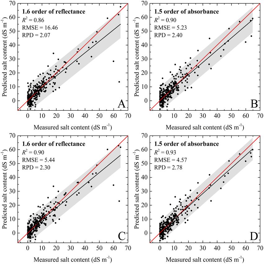
China is affected by salinity (Peng et al., 2016; Wang et al., 2007). Oasis ecosystem is the
                                   material and ecological base of arid and semi-arid areas (Abliz et al., 2016). With the rapidly
                                   increasing population densities and drastic land use changes over the past few decades,
                                   soil salinization has become the main restraint not only for a sustainable development
                                   of oasis agriculture, but also for the stability of regional ecosystems (Scudiero, Skaggs &
                                   Corwin, 2014). Timely detection as well as assessment of soil salinity are essential to regional
                                   ecological stability, and these problems have attracted considerable attention worldwide in
                                   recent years.
                                      Traditionally, the detection and assessment of soil salinity require intensive field-derived
                                   work, e.g., the electromagnetic measurements of soil electrical conductivity (EC) or time-
                                   consuming laboratory experiments (Ding & Yu, 2014). In-situ measurements have been
                                   widely proved to be the most valid approach to assess soil salinity; however, they could
                                   only provide limited point information, rather than large-scale spatial global information
                                   (Dehaan & Taylor, 2002). Compared to conventional laboratory analysis methods, the
                                   remote sensing technology is a promising alternative approach for quantitative evaluation
                                   of soil attributes due to its obvious characteristics, including rapid response, low cost,
                                   wide view filed, and fast acquisition (Ben-Dor & Banin, 1995; Farifteh, Farshad & George,
                                   2006; Metternicht & Zinck, 2003). Remote sensing data is well-adopted for mapping and
                                   assessing various characteristics of surface soil across different scale (Allbed, Kumar &
                                   Aldakheel, 2014; Corwin et al., 2003). Therefore, based on the different spectral reflection
                                   and absorption characteristics of the VIS–NIR bands to soil salinity, spectral analysis
                                   technology could be an alternative to ensure accurate estimation of salt content in soils.
                                   (Cécillon et al., 2009; Islam, Singh & McBratney, 2003).
                                      The applicability of VIS–NIR has been investigated and the results showed that the
                                   characteristic bands cover the absorption spectra of NaCl (1,930 nm), KCl (1,430 nm),
                                   and MgSO4 (1,480 nm) (Cécillon et al., 2009; Stenberg et al., 2010). The different spectral
                                   reflection and absorption characteristics of the VIS–NIR bands to soil salinity laid the
                                   foundation of quantifying soil salinity. The partial least squares regression (PLSR) and
                                   artificial neural network (ANN) have been successfully used for predicting main salt
                                   concentrations of soils using reflectance spectroscopy (Farifteh et al., 2007). Using raw
                                   reflectance and pretreatment by Savitzky–Golay (S-G) smoothing, first derivative (FD) and
                                   second derivative (SD), the performance of PLSR, and multivariate adaptive regression
                                   splines (MARS) were compared to identify the best regression approach to quantify soil
                                   salinity (Nawar, Buddenbaum & Hill, 2015). Viscarra Rossel & Behrens (2010) compared
                                   the performance of PLSR, ANN, random forest (RF) and five other different data mining
                                   algorithms for the assessment of organic carbon (OC), clay content and pH of soil.
                                   Because it can consider dimension synthesis and solve the multiple collinearity problems
                                   among independent variables, PLSR is a frequently used and reliable linear regression
                                   method especially for quantitative research (Llndber, Persson & Wold, 1983; Wold, Sjöström
                                   & Eriksson, 2001). This technology has proved to be capable of inference capabilities, which
                                   could simulate the potential linear relationship between some specific soil attributes and
                                   corresponding VIS–NIR reflectance (Farifteh et al., 2007; Nawar et al., 2014).

Wang et al. (2018), PeerJ, DOI 10.7717/peerj.4703                                                                             2/24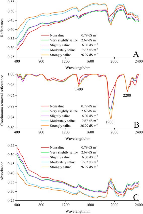
However, the non-uniform data distribution and non-linear reflectance behavior
                                   indicate that the application of PLSR is insufficient, which has some limitations (Nawar et
                                   al., 2016). The RF is an ensemble machine learning technique with the capability of solving
                                   classification, regression, and other tasks in different fields (Breiman, 2001). Differing from
                                   existing linear and non-linear regression modeling methods, RF has acceptable predicting
                                   performance even if most independent variables are noise (Chen & Liu, 2005). Owning
                                   to its higher quality implementations, fewer restrictions and excellent performance, RF
                                   has been widely used in bioinformatics, hyperspectral data classification and other related
                                   disciplines, and generally exhibits higher accuracy and efficiency (Díaz-Uriarte & Alvarez de
                                   Andrés, 2006; Pal, 2005; Rodriguez-Galiano et al., 2012; Shi & Horvath, 2006; Sun & Schulz,
                                   2015). Numerous studies have demonstrated that RF provided better spectral estimations
                                   than those by PLSR (Clark, Roberts & Clark, 2005; Douglas et al., 2018; Stevens et al., 2013;
                                   Viscarra Rossel & Behrens, 2010). As a source of high-dimensional data, spectral reflectance
                                   data possess high spectral resolution, consecutive wavebands, and a variety spectral
                                   information (Wang et al., 2017b). Quantifying soil salinity with VIS–NIR reflectance is
                                   therefore challenging, due to the large amount of irrelevant spectral data and inherent
                                   noise. Furthermore, a defect of signal-to-noise ratio decreasing at longer wavelengths
                                   might affect the deep application from VIS–NIR spectroscopy. In the study of estimating
                                   soil parameters reported previously, spectral reflectance has been applied directly, and the
                                   relationship between integer derivative transforms (FD and SD) of spectral data and the salt
                                   content or EC of soils has been well studied (Nawar, Buddenbaum & Hill, 2015; Shi et al.,
                                   2013; Viscarra Rossel & Webster, 2012). However, the detection of spectral information via
                                   FD and SD with wider order intervals could, to some degree, result in the loss of spectral
                                   information. Some studies have demonstrated significant improvements on potential
                                   applications of the fractional derivative in various fields (Chen, 2008; Wang et al., 2017a;
                                   Wang et al., 2017c; Zhang et al., 2016a). With the narrower order interval, the fractional
                                   derivative expanded the theoretical concept of classic derivative. It has proved to be an
                                   effective pretreatment of spectral data (Wang et al., 2017b; Zhang et al., 2016a). Moreover,
                                   the algorithm has been used for preprocessing the spectral data of soils, and the results
                                   demonstrated that it could improve the sensitivity between the dependent and independent
                                   variables in the spectral analysis (Xia et al., 2017).
                                       Although some existing researches have estimated local soil salinity and clay content
                                   using VIS–NIR preprocessed by fractional derivative, accurate and stable fractional order
                                   for the ideal estimation have not been implemented yet (Wang et al., 2017b; Zhang et al.,
                                   2016a). Substantial efforts in predicting soil salinity suffer from the limitations of different
                                   modeling approaches to provide a generalized model over various scales and datasets.
                                   This study aimed to fill the gap and to advance the use of VIS–NIR for quantifying soil
                                   salinity based on the pretreatment of fractional derivative. The main objectives of this
                                   study were (1) to establish a generalized stable model to predict soil salinity by means of
                                   VIS–NIR spectroscopy; (2) to select the optimal fractional derivative order for soil salinity
                                   estimation; (3) to compare linear (PLSR) and non-linear (RF) models for the most effective
                                   quantitative prediction of soil salinity.

Wang et al. (2018), PeerJ, DOI 10.7717/peerj.4703                                                                             3/24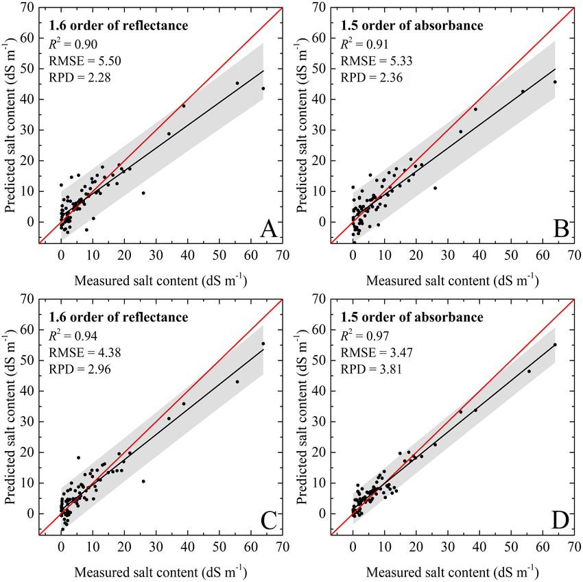
MATERIALS AND METHODS
                                   Study area
                                   The Ebinur Lake wetland, a core area of Oasis–Desert System in Central Asia, was selected
                                   as the study area. Ebinur Lake is located in the south-western region of the Junggar
                                   Basin (44◦ 200 ∼45◦ 290 N, 82◦ 060 ∼83◦ 400 E, northwestern XUAR) (He et al., 2015; Liu et al.,
                                   2011). The total area of the study area is 2,670.8 km2 (Ge et al., 2016). The wetland has
                                   a typical temperate continental climate with scarce precipitation (100–200 mm), strong
                                   potential evaporation (≥1,600 mm) and strong winds (≥8 m/s, on 164 days) annually.
                                   The soil salinity of the study area varies from very slightly saline to strongly saline and local
                                   prevalent salt minerals are NaCl (Liu et al., 2011). According to the World Reference Base
                                   for Soil Resources (WRB), local prevalent soil types are mainly Arenosols, Solonetz, and
                                   Solonchaks (Deckers et al., 2002; He et al., 2015). The study area is characterized by fragile
                                   ecology and is particularly sensitive to climate change and human activities. In recent years,
                                   the drawdown of dry lakebed (playa) has exposed broad hard salt crusts and saline desert,
                                   which might have a range of negative effects on the local fragile environment (Liu et al.,
                                   2011). To protect the important wetland ecosystems in arid areas, the Chinese government
                                   has designated the adjoining of the Ebinur Lake wetland as a National Nature Reserve in
                                   April 2007 (Zhang et al., 2016b).

                                   Sample collection and chemical analysis
                                   To ensure the relative representative and homogeneous soil types, soil texture and
                                   landscape, the samples were obtained from a total of 100 sampling units on a grid of 30 m
                                   × 30 m (because the spatial resolution of Landsat satellite imagery is 30 m) throughout
                                   the study area in October 2016 (Fig. 1). A portable GPS meter (Garmin GPS 72) was
                                   employed to record the coordinates of each sampling point, as displayed in Fig. 1E. In each
                                   unit, about 0.50 kg of topsoil from depths of 0 to 5 cm was collected at four randomly
                                   selected sampling sites. Each sample was placed into a sealed watertight bag and labeled.
                                   A total of (4 × 100) topsoil samples were obtained and preserved for the soil attributes
                                   measurements. All samples were sufficiently air-dried (over 35 ◦ C) for two weeks, ground,
                                   and then passed through a 2.0 mm sieve to wipe off plant materials, residue, and stones.
                                   Prior to chemical analysis, organic carbon (OC) was removed using hydrogen peroxide
                                   (H2 O2 , 30%). We determined the soil salinity and pH value with a digital multiparameter
                                   measuring apparatus (Multi 3420 Set B, WTW GmbH, Germany) equipped with the
                                   composite electrode (TetraCon 925 and SenTix 940) in a 1:5 soil-water extraction solution
                                   at room temperature (25 ◦ C). The measurement of soil particle size was conducted using
                                   a particle analyzer system (Bluewave S3500, Largo, FL, USA). Seven main soluble ions
                                   concentrations, i.e., potassium (K+ ), sodium (Na+ ), calcium ion (Ca2+ ), magnesium ion
                                                                                                        −
                                   (Mg2+ ), chloridion (Cl− ), sulphane (SO2−
                                                                            4 ) and mbicarbonate (HCO3 ) were also evaluated
                                   according to the standardized method outlined by Bao (2000). The concentrations of K+
                                   and Na+ were measured using flame photometry method; Ca2+ and Mg2+ were measured
                                   using EDTA complexometric titration method; Cl− was determined using the silver nitrate
                                   (AgNO3) titration method; SO2−   4 was determined by the EDTA indirect titration method;

Wang et al. (2018), PeerJ, DOI 10.7717/peerj.4703                                                                              4/24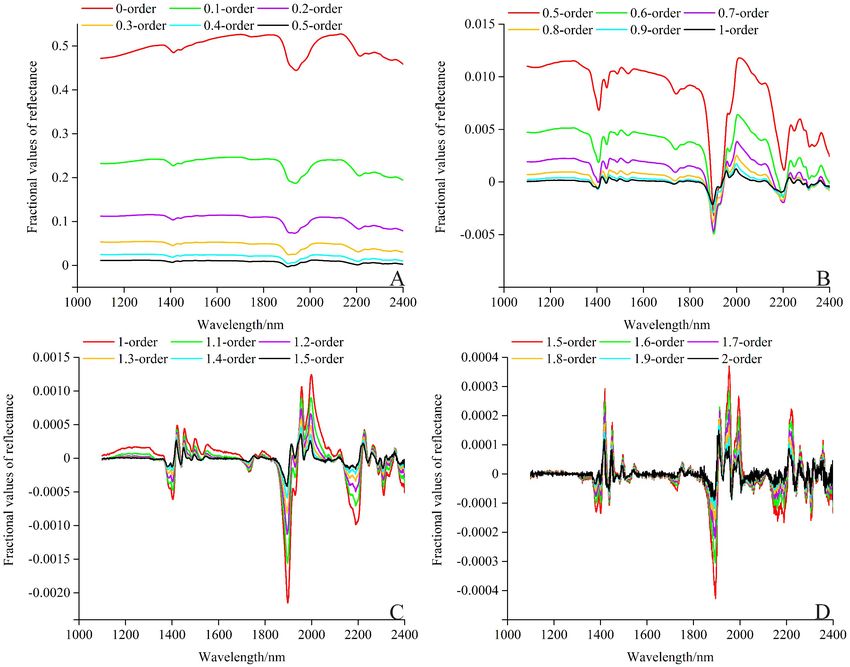
Figure 1 Distribution of sampling sites in the study area. (A) Location map of XUAR. (B) Ebinur Lake
                                    wetland region. (C and D) Typical landscape photograph (Photograph credit: Jingzhe Wang). (E) The
                                    schema of sampling method (4 points) within the 30 m × 30 m cell grid.
                                                                                                   Full-size DOI: 10.7717/peerj.4703/fig-1

                                   HCO− 3 was determined using the double indicator neutralisation method. The detailed
                                   description of main soil physicochemical attributes is given in Table 1.

                                   Spectral measurements under laboratory conditions and
                                   pretreatment
                                   The VIS–NIR spectroscopic measurements in laboratory were conducted using a portable
                                   FieldSpec R 3 ASD Spectroradiometer device with a resampling interval of approximately
                                   1.0 nm in the measurement range (350–2,500 nm). The sampling intervals of the device are
                                   1.4 nm and 2 nm, in the 350–1,000 nm range, and 1,000–2,500 nm range, respectively. Prior
                                   to spectrum measurements, each soil sample was placed into a petri dish in the dark (12 cm
                                   diameter, 1.8 cm depth) (Peng et al., 2014). The detailed measurement conditions of the
                                   step were given by Wang et al. (2017b). To avoid biased measurements, the spectrometer
                                   was corrected with a calibrated Spectralon R panel with near 100% reflectance before
                                   the spectral measurement. Ten spectral curves were gathered, and then averaged as the
                                   final reflectance value. To minimize the effect of inherent spectral noise at the edges of
                                   spectra, the reflectance was reduced to 400–2,400 nm. Because of the slight fluctuations
                                   in the spectral reflectance, the Savitzky–Golay (S-G) algorithm was adopted in spectral
                                   smoothing and realized the two order polynomial fit in the window size of five data
                                   points (Savitzky & Golay, 1964). Subsequently, subjecting the spectra subset (400–2,400
                                   nm range) to SG smoothing and absorbance (–lg R, R meaning the reflectance) processing.
                                   They comprised the data source of spectral analysis and model construction in this study
                                   and are provided as Table S1.

Wang et al. (2018), PeerJ, DOI 10.7717/peerj.4703                                                                                     5/24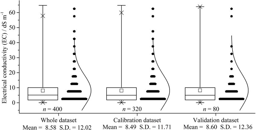
Table 1 Main physicochemical attributes of soil samples in the study area (mean ± S.D.).

                                     Item                                         Unit                                     Value
                                     Sand                                         %                                        75.31 ± 17.68
                                     Silt                                         %                                        23.35 ± 16.63
                                     Clay                                         %                                        1.34 ± 1.17
                                     Main texture                                 /                                        Sandy Loam
                                     EC                                           dS m−1                                   8.58 ± 12.02
                                     pH                                           /                                        8.35 ± 0.42
                                     K+                                           g kg−1                                   0.38 ± 0.04
                                          +                                           −1
                                     Na                                           g kg                                     18.30 ± 2.65
                                     Ca2+                                         g kg−1                                   4.33 ± 0.46
                                     Mg2+                                         g kg−1                                   0.43 ± 0.07
                                     HCO−
                                        3                                         g kg−1
                                                                                                                           2.13 ± 1.33
                                      −
                                     Cl                                           g kg−1                                   6.25 ± 12.63
                                     SO2−
                                       4                                          g kg−1
                                                                                                                           13.98 ± 15.02
                                   Notes.
                                       S.D., indicates standard deviation.

                                   Grünwald-Letnikov fractional derivative
                                   The application of derivatives is an ideal treatment in spectral analysis (Viscarra Rossel,
                                   McGlynn & McBratney, 2006). The VIS–NIR reflectance was derivative-converted to reduce
                                   the influence of noise, amplify and reveal the greater spectral features (Wang et al., 2017a).
                                   The fractional derivative has expanded the theoretical concept of classic derivative, which
                                   has been successfully adopted in spectral data processing. To reduce the complexity of the
                                   discrete operation, the Grümwald–Letnikov definition of fractional derivative algorithm
                                   was employed for the calculations in the current study. A detailed description of the
                                   definitions is available in previous publications (Xia et al., 2017; Zhang & Chen, 2015).
                                   When the order is set as α, the α-order fractional derivative of function f (x) on the section
                                   of [ β, γ ] is as follows:
                                                   [(t−a)/h]
                                     α            1 X                0(α + 1)
                                   d f (x) = lim α          (−1)m                f (x − mh)                                               (1)
                                             h→0 h                m!0(α − m + 1)
                                                              m=0

                                   where h represents step length, and [(γ − β)/h] represents integer part of (γ − β)/h.
                                     The Gamma function is defined as:
                                          Z ∞
                                   0(z) =     exp(−u)uz−1 du = (z − 1)!                                                  (2)
                                               0
                                      Based on the actual resampling interval of the spectral sensor is 1 nm, then set h = 1, Eq.
                                   (1) can be written as follows:
                                   d α f (x)                           (−α)(−α + 1)                       0(−α + 1)
                                         α
                                             ≈ f (x) + (−α)f (x − 1) +              f (x − 2) + ······                 f (x − n).
                                     dx                                     2                          n!0(−α + n + 1)
                                                                                                                               (3)

                                      Therefore, Eq. (3) can be considered as the specific formula for the calculation in this
                                   study. It is noted that the 0.0 order means that the data are not processed, which means

Wang et al. (2018), PeerJ, DOI 10.7717/peerj.4703                                                                                        6/24
the raw value (Hollkamp, Sen & Semperlotti, 2017). According to Eq. (3), set order interval
as 0.1, fractional derivatives of reflectance and their absorbances, range from the 0.0 to the
2.0 order were calculated in the current study,
Model calibration, evaluation, and comparison
The PLSR and RF were applied to establish models for soil salinity quantitative estimation
from pretreated VIS–NIR reflectance (400–2,400 nm range). In this section, to ensure the
full range of soil salinity is represented in both dataset, we used the Kennard-Stone (K-S)
algorithm for samples selection (Wang et al., 2017b). The whole dataset (n = 400) was split
into two sections: 80% for calibration (cross-validation, n = 320) and 20% for prediction
(independent validation, n = 80).
Partial least squares regression (PLSR)
The PLSR has been frequently used in spectral quantitative research due to its superiority
of dimension reduction and the synthesis. Detailed description of PLSR is available in
Wold, Sjöström & Eriksson (2001). In the calculation procedure of the step, PLSR follows
a linear multivariate model to associate the independent variables (X, reflectance in this
research) and dependent variables (Y, soil salinity in this research) and select latent factors
(variables). Thereby, it compresses X variables into a small number of latent variables
(LVs) to maximize the covariance between the LV scores and Y variables. To identify the
ideal number of LVs, leave-one-out cross validation (LOOCV) was conducted. Parameter
optimization and modeling were implemented with the PLS_Toolbox (version 7.9) based
on MATLAB R software version R2012a (MathWorks, Inc., Natick, MA, USA).
Random forest (RF)
The RF, a recently prevalent machine learning method for classification and regression,
can estimate complicated non-linear relationships between independent variables and
response variables (Pal, 2005; Wang et al., 2018). It has proved a promising regression
method especially in estimating soil attributes using VIS–NIR (Shi & Horvath, 2006). The
RF aggregates various predictions based on changes in the training dataset through
resampling. This algorithm consists of an ensemble of stochastic classification and
regression trees (CART). Consequently, RFs are developed based on a combination of
bagging method and randomized subspace method and then applied at each split in the
tree. To grow each tree, the size of the variables subset (mtry) has to be selected by the user.
Each decision tree grows until reaching a predefined minimum number of nodes (nodesize)
on the new training dataset via random feature selection. In this research, the number of
trees (ntree) was set to 500, both the size of the variables subset (mtry) and the minimum
number of nodes (nodesize) were set to 2. The parameter selection and regression were
conducted using Random Forest package (version 4.6-12) based on R software (version
3.4.0) (Douglas et al., 2018; Liaw, 2002).
Model evaluation and comparison
Two models, PLSR versus RF, were constructed and cross-validated with the training
dataset, and independently validated via the testing dataset, separately. For the assessment
Wang et al. (2018), PeerJ, DOI 10.7717/peerj.4703 7/24Figure 2 Flow chart of the study.
Full-size DOI: 10.7717/peerj.4703/fig-2
of performance of spectroscopic models: (1) the coefficients of determination (R2 ), (2)
root mean square errors (RMSE), and (3) ratio of performance to deviation (RPD) were
calculated and compared individually. The definitions and formulae for the indices were
given by Shi et al. (2014).
Based on the estimating model classification criterion illustrated by Viscarra Rossel et
al. (2006), the inversion models could be partitioned into six classifications: Category A
(RPD ≥ 2.50) is the excellent model; Category B (2.00 ≤ RPD < 2.50) is the very good
quantitative model; Category C (1.80 ≤ RPD < 2.00) is the good model, the quantitative
estimation might be possible; Category D (1.40 < RPD ≤ 1.80) is the fair model with
limited performance; Category E (1.00 < RPD ≤ 1.40) is the poor model, which could
only distinguish the difference of the high and low levels; Category F (RPD ≤ 1.00) is the
unreliable model. Generally, optimal models with highest R2 (approach to 1) and RPD but
lowest RMSE (approach to 0) would be selected.
The steps of model construction and validation are illustrated in Fig. 2.
RESULTS
Descriptive statistical analysis
The soil salinity of the study area varied widely between 0.03 and 64.80 dS m−1 , with an
average salinity of 8.58 dS m−1 , standard deviation of 12.02 dS m−1 , and a high coefficient
of variation of 140.87% (>100%) (Fig. 3). The relative high mean salinity indicated that
the surface soils were salt-affected in the Ebinur Lake wetland. Compared to the range of
the salinity (0.03–64.80 dS m−1 ) for the calibration dataset, the validation dataset had a
similar range of 0.06–63.42 dS m−1 with mean and standard deviation of 8.60 dS m−1 and
12.36 dS m−1 , respectively. The results showed that the distribution of the soil salinity of all
datasets was left-skewed in contrast to the standardized normal distribution. The statistical
Wang et al. (2018), PeerJ, DOI 10.7717/peerj.4703 8/24Figure 3 Box plot and distribution of soil salinity for the whole, calibration, and validation dataset (dS
m −1 ). S.D. indicates standard deviation.
Full-size DOI: 10.7717/peerj.4703/fig-3
results of soil salinity in both calibration and validation dataset were similar to those of
the whole dataset; consequently, the soil salinity of both datasets adequately represent the
entire dataset.
Reflectance of different soil salinity
Based on the standard of different soil salinity level outlined by the United States
Department of Agriculture (USDA), all 400 samples were classified into five different
classes of soil salinity: non-saline (0–2 dS m−1 ), very slightly saline (2–4 dS m−1 ), slightly
saline (4–8 dS m−1 ), moderately saline (8–16 dS m−1 ), and strongly saline (>16 dS m−1 )
(Schoeneberger et al., 2002; Shahid & Rehman, 2011). The soil reflectivity and spectral
features vary with the different level of soil salinity (Fig. 4A). As seen in the diagram,
spectral curves of soil with different salinity followed a similar shape. Notably, there were
significant differences between moderately saline, strongly saline, and the other three
degrees of soil salinity.
The continuum removal (CR) technique ordinarily can restrain the noise of background
and emphasize weak absorption features in the spectra (Ji et al., 2014). The corresponding
CR reflectance are illustrated in Fig. 4B. The three main absorption features were located
at around 1,400, 1,900, and 2,200 nm, respectively. The absorption features at 1,400 nm
are a representative absorption region for water combined with the bending and stretching
vibration of the O-H bonds of free water (Shi et al., 2014). The regions near 1,900, and
2,200 nm in the combination range exist due to the bending and stretching vibrations of
Al–OH and Mg–OH, respectively (Pu et al., 2003; Viscarra Rossel, McGlynn & McBratney,
2006a). Considering the essence of absorbance (−lg R), the absorbance curves are the
reversal of spectral curves (Figs. 4A and 4C).
Wang et al. (2018), PeerJ, DOI 10.7717/peerj.4703 9/24Figure 4 Reflectance spectra curves of soils with different salinity degrees. (A) Spectral curves. (B)
Continuum removal curves. (C) Absorbance curves.
Full-size DOI: 10.7717/peerj.4703/fig-4
Wang et al. (2018), PeerJ, DOI 10.7717/peerj.4703 10/24Table 2 Results of leave-one-out cross validation for PLSR of both reflectance and absorbance treated by fractional derivatives.
Order Reflectance Absorbance
2 2
Latent R RMSE RPD Latent R RMSE RPD
variables (dS m−1 ) variables (dS m−1 )
0.0 4 0.64 9.27 1.30 3 0.58 9.80 1.23
0.1 4 0.66 9.07 1.33 4 0.63 9.37 1.29
0.2 4 0.69 8.75 1.38 4 0.68 8.90 1.36
0.3 4 0.71 8.56 1.42 4 0.67 8.98 1.35
0.4 5 0.77 7.77 1.57 4 0.68 8.90 1.36
0.5 2 0.54 10.08 1.19 2 0.52 10.27 1.17
0.6 2 0.56 9.93 1.21 2 0.55 10.03 1.20
0.7 5 0.81 7.20 1.70 3 0.67 8.97 1.35
0.8 3 0.71 8.49 1.43 3 0.66 9.04 1.34
0.9 3 0.72 8.43 1.44 3 0.68 8.87 1.36
1.0 3 0.70 8.70 1.39 3 0.66 9.05 1.34
1.1 5 0.84 6.63 1.86 5 0.79 7.43 1.65
1.2 5 0.84 6.76 1.82 5 0.82 7.03 1.75
1.3 5 0.84 6.73 1.83 5 0.84 6.68 1.84
1.4 5 0.84 6.36 1.94 5 0.84 6.18 1.99
1.5 5 0.84 6.18 2.01 5 0.87 5.23 2.40
1.6 5 0.86 6.00 2.07 5 0.84 6.06 2.05
1.7 5 0.85 6.16 2.02 5 0.84 6.07 2.04
1.8 5 0.84 6.19 2.00 5 0.83 6.09 2.03
1.9 5 0.84 6.73 1.83 5 0.83 6.85 1.79
2.0 5 0.83 6.85 1.79 5 0.83 6.98 1.76
Influence of spectral preprocessing methods
In the current study, all spectral reflectance data and according absorbances preprocessed by
the fractional derivative were used for the model construction. Various fractional derivative
orders had significant effects on the outcomes of soil salinity estimating models (Table 2).
Compared with the PLSR models based on 0.0 order (without pretreatment of fractional
derivative), besides the 1.4 order of absorbance, 1.5–1.8 orders of reflectance and absorbance
improved the accuracies (RPD ≥ 2.00). The model based on the 1.5 order of absorbance
possessed the optimum estimation performance (R2 = 0.87, RMSE = 5.23 dS m−1 , and
RPD = 2.40). In contrast, the pretreatment of 0.5 order fractional derivative resulted in
the least acceptable results (R2 = 0.54 and 0.52, RMSE = 10.08 dS m−1 and 10.27 dS m−1 ,
and RPD = 1.19 and 1.17 for reflectance and absorbance models, respectively). Excluding
it, the PLSR models built on fractional derivative outperformed those using the classic
integer derivatives (FD and SD). However, the parameters did show gradual improvement
with the increase from the order 1.0 to 1.5. With increasing order, the RMSE and RPD
values of the models gradually decreased. As the order increased to 1.5, the performance
of the model improved drastically (Table 2). Thereby, the calibrations of the eight spectral
methods achieved desirable performances with PLSR (1.5-order, 1.6-order, 1.7-order, and
Wang et al. (2018), PeerJ, DOI 10.7717/peerj.4703 11/241.8-order based on reflectance, and 1.5-order, 1.6-order, 1.7-order, and 1.8-order based
on absorbance, respectively) and were used for the model construction.
Performance of PLSR and RF models for salinity quantitative
estimation
In this research, different calibration methods produced various estimation accuracies
for soil salinity. For the calibration dataset of PLSR, the predicting model based on
the absorbance (1.5 order) had the best performance (R2C = 0.90, RMSEC = 5.23 dS
m−1 , and RPDC = 2.40), while the worst results were with the 1.8 order of reflectance
(R2C = 0.85, RMSEC = 6.19 dS m−1 , and RPDC = 2.00). Except for the 1.6 order,
PLSR models based on the fractional derivative orders of absorbance outperformed
the according reflectance models at the same order (Figs. 5A and 5B). Compared
to PLSR, the RF models had better performances than the PLSR models with each
preprocessing technique, and RPD ranged from 2.00 to 2.78. The RF model based on
the absorbance (1.5 order) possessed the best capability (R2C = 0.93, RMSEC = 4.57
dS m−1 , and RPDC = 2.78), followed by the model based on the 1.6 order. In
addition, all calibration models had very good RPD values exceeding 2.00 for the
above eight spectral pre-processing methods (Tables 3 and 4; Figs. 5C and 5D).
With respect to the validation dataset, it had similar variation trends compared to those
of the calibration dataset, but had higher prediction accuracies. For the PLSR model,
the validation results with the 1.5 order of absorbance was most accurate (R2V = 0.91,
RMSEV = 5.33 dS m−1 , and RPDV = 2.36). The RF models with all spectral preprocessing
produced good performance, and the RPD values were close to or even greater than 2.50.
The RF models with the 1.5 order of absorbance showed excellent performance (R2V = 0.97,
RMSEV = 3.47, and RPDV = 3.81 ≥ 2.50). The validation accuracies of PLSR models were
slightly lower than those of RF, but still very good for the soil salinity quantitative estimation
(R2V = 0.89–0.91, RMSEV = 5.33–5.89 dS m−1 , and RPDV = 2.19–2.36). For the validation
dataset, the slopes for the PLSR and RF models based on 1.6 order of absorbance were well
distributed to the 1:1 line which indicated excellent validations. However, the slopes for
the PLSR and RF models based on 1.5 order of reflectance were under the 1:1 line, and
the data points were relatively discrete (Tables 3 and 4; Fig. 6). In addition, some negative
values were recorded in the prediction results.
DISCUSSION
Fractional derivative results of the reflectance
Fractional order derivative processing influences the spectral data to a certain degree
(Schmitt, 1998). The fractional derivative results of the average reflectance in the range of
1,100–2,400 nm (long-wavelength near-infrared spectroscopy, LW–NIR) are illustrated in
Fig. 7. With the order increasing from 0.0 to 1.0, the fractional derivative curves slowly
followed the FD (1.0 order) curve, and became sensitive to the slope and less sensitive
to reflectance. From 1.0 to 2.0, the fractional derivative curves slowly approached the SD
(2.0 order) curve and, to a certain extent, became more sensitive to the curvature and less
sensitive to the slope (Wang et al., 2017a). The fractional derivative results of the reflectance
Wang et al. (2018), PeerJ, DOI 10.7717/peerj.4703 12/24Figure 5 The soil salinity quantitative models using calibration dataset. (A) PLSR model based on 1.6
order of reflectance. (B) PLSR model based on 1.5 order of absorbance. (C) RF model based on 1.6 or-
der of reflectance. (D) RF model based on 1.5 order of absorbance. The black line represents the fitted
line, the red line represents the 1:1 line, and the gray regions represent the confidence intervals with 95%
probability.
Full-size DOI: 10.7717/peerj.4703/fig-5
showed a fluctuating trend in this region. Some less obvious absorption peak information
was magnified. The strengthening of peak intensity in VIS–NIR was very important to
the further exploration of its reflection mechanism (Li et al., 2014). Compared with the
conventional raw reflectance, FD, and SD, more spectral characteristics were refined of the
spectrum reflectance treated by the pretreatment of fractional derivative, and are provided
as Table S2.
Effects of fractional derivative on estimation models
Due to the abundant spectral information and the rapid data acquisition, VIS–NIR has been
frequently used for assessing multiple soil parameters. To obtain more spectral information
Wang et al. (2018), PeerJ, DOI 10.7717/peerj.4703 13/24Table 3 The cross validation of the calibration dataset (n = 320) and the capability of the validation
dataset (n = 80) for the quantitative estimation of soil salinity using PLSR model with different spectral
types.
Spectral types Order Calibration dataset Validation dataset
R2 RMSE RPD R2 RMSE RPD
(dS m−1 ) (dS m−1 )
1.5 0.86 6.18 2.00 0.90 5.63 2.22
1.6 0.86 6.00 2.07 0.90 5.50 2.28
Reflectance
1.7 0.85 6.16 2.01 0.90 5.60 2.24
1.8 0.85 6.19 2.00 0.89 5.89 2.12
1.5 0.90 5.23 2.40 0.91 5.33 2.36
1.6 0.84 6.06 2.05 0.91 5.36 2.35
Absorbance
1.7 0.84 6.07 2.04 0.90 5.44 2.31
1.8 0.85 6.09 2.03 0.89 5.71 2.19
Table 4 The cross validation of the calibration dataset (n = 320) and the capability of the validation
dataset (n = 80) for the quantitative estimation of soil salinity using RF model with different spectral
types.
Spectral types Order Calibration dataset Validation dataset
2 2
R RMSE RPD R RMSE RPD
(dS m−1 ) (dS m−1 )
1.5 0.87 6.11 2.00 0.90 5.57 2.26
1.6 0.90 5.44 2.30 0.94 4.38 2.96
Reflectance
1.7 0.90 5.57 2.24 0.91 5.41 2.34
1.8 0.89 5.63 2.22 0.90 5.58 2.26
1.5 0.93 4.57 2.78 0.97 3.47 3.81
1.6 0.90 5.42 2.30 0.93 4.72 2.71
Absorbance
1.7 0.90 5.49 2.26 0.92 5.10 2.49
1.8 0.88 5.55 2.25 0.91 5.23 2.42
and features and to further improve the robustness and capability of the models, it is vital
to preprocess raw reflectance (Nawar et al., 2016). Spectral derivative analysis is a simple
and effective preprocessing method which is commonly used for the enhancement of
spectral information. In general, the order interval is set to 1.0, and the regression models
are constructed based on the FD or SD. However, pretreatment of the FD and SD might
cause the loss of spectral information (Wang et al., 2017a). In this research, raw reflectance
and absorbance without pretreatment (0.0 order) and the corresponding FD and SD were
applied for the model construction as well. For reflectance, the PLSR model based on 0.0
order is poor with the lower RPD (1.30 ≤ 1.40). Once the order reached 1.0 (FD), the
quantifying capability slightly improved; however, it was not suitable for the quantitative
estimation of soil salinity (R2 = 0.70, RMSE = 8.70 dS m−1 , and RPD = 1.39 ≤ 1.40).
With regard to SD, the corresponding model with a value of RPD = 1.79 ≤ 2.00 was better
than the models based on FD, and still retained an inadequate prediction ability; hence,
it was unsuitable for quantitative estimation. In the current study, the various fractional
Wang et al. (2018), PeerJ, DOI 10.7717/peerj.4703 14/24Figure 6 The soil salinity quantitative models using validation dataset. (A) PLSR model based on 1.6
order of reflectance. (B) PLSR model based on 1.5 order of absorbance. (C) RF model based on 1.6 or-
der of reflectance. (D) RF model based on 1.5 order of absorbance. The black line represents the fitted
line, the red line represents the 1:1 line, and the gray regions represent the confidence intervals with 95%
probability.
Full-size DOI: 10.7717/peerj.4703/fig-6
derivative orders significantly affected the results of soil salinity calibration models (Table
2). In addition, the variation trend of the precision parameters was obvious; where the
model was based on the 0.5 order, it showed the worst performance with the lowest
RPD (1.19) and the highest RMSE (10.08 dS m−1 ). In comparison, the accuracies of the
calibrition models based on absorbance were slightly weaker than those of the reflcetance
models, while the condition of the validation data sets showed an inverse pattern. The
preprocessing of the 1.6 order of absorbance obtained the best performance followed by
the 1.5 order of reflectance.
Wang et al. (2018), PeerJ, DOI 10.7717/peerj.4703 15/24Figure 7 Fractional derivative results of the reflectance in the range of LW–NIR (1,100–2,400 nm). (A)
0–0.5 order. (B) 0.5–1.0 order. (C) 1.0–1.5 order. (D) 1.5–2.0 order.
Full-size DOI: 10.7717/peerj.4703/fig-7
Our results showed that the 1.5 order of absorbance was the optimal fractional derivative
order for PLSR and RF based estimation of soil salinity. The pretreatment of fractional
derivative orders has also been applied in previous research to model various soil properties
(Wang et al., 2017a; Zhang et al., 2016a). For example, Wang et al. (2017b) applied the
fractional derivative algorithm for the pretreatment of the reflectance of soil, and the PLSR
results were effectively improved.
Compared to the common integer derivative (FD and FD), the preprocessing of
fractional derivative with a narrower order interval could collect more details and features
from spectra and further lay the foundation for the improvement of the capability of the
predecting models.
Comparison between PLSR and RF models in estimating soil salinity
In the current study, the PLSR and RF were applied for the quantitative estimation of
soil salinity of the Ebinur Lake wetland. The two techniques showed different accuracies
depending on the different type of reflectance. Between the two calibration methods,
RF was statistically superior to PLSR, while PLSR provided slightly weaker predictive
power. Compared with existing results obtained using PLSR (R2 = 0.66–0.87) and RF
(R2 = 0.78–0.91), the soil parameters models developed in the current study could be
Wang et al. (2018), PeerJ, DOI 10.7717/peerj.4703 16/24regarded as acceptable under the classification standard (Islam, Singh & McBratney, 2003;
Nawar et al., 2014; Shepherd & Walsh, 2002; Shi et al., 2014; Wang et al., 2018; Wang et al.,
2017b; Zhang et al., 2016a). The PLSR technique could effectively solve multiple collinearity
problems among independent variables, but only simulate the potential linear relationship
between some specific soil attributes and corresponding VIS–NIR reflectance. In reality, the
distribution of soil properties is mostly skewed distribution rather than the standardized
normal distribution, and the application of linear regression method such as PLSR may
be insufficient. Thereby, the RF model typically yields superior estimation accuracies if a
non-linear relationship exists between predictor and response variables.
RF recorded the excellent validation accuracies based on the effective preprocessing
method with ideal R2 (0.90–0.97), RMSEV (3.47–5.57 dS m−1 ), and all RPD greater than
2.00 (Table 4). Compared to the validation accuracy, the performance of calibration was
slightly lower but still acceptable (R2 between 0.87 and 0.93, RMSEV between 4.57–6.11 dS
m−1 ), RPD between 2.00 and 2.78). In terms of RPD, the best RF model was calibrated with
the 1.5 order of absorbance, and the optimal model performance was obtained (R2 = 0.93
and RMSEC = 4.57 dS m−1 ). For the validation dataset, the PLSR model with the same
pretreatment method performed relatively well across the seven models except in the case
of the 1.5 order of absorbance model (RMSEV = 5.23 dS m−1 , RPD = 2.40; Table 3).
However, the calibration dataset of soil salinity had an extremely wide range, varying from
0.03 to 64.80 dS m −1 with a standard deviation value of 12.10 dS m−1 , and included some
samples of non-saline soil. The high accuracies of PLSR and RF with validation dataset
might be attributed to the data distribution (88.750% of soil samples were saliferous). Zhang
et al. (2016a) set the order interval to 0.2 and indicated that the model constructed by 250
feature bands based on 1.2-order derivative of absorbance possessed an excellent capacity
of estimating soil salinity. Generally, the pretreatment of fractional derivative could refine
and enhance the spectral characteristics of the spectrum reflectance (Wang et al., 2017c).
Compared with the previous studies, the combination of RF and narrower fractional order
interval could significantly improve the estimations accuracies and generalization ability.
Research limitations
The superior performance of RF in comparison with the PLSR models tested could be
explained by its outstanding ability to deal with the non-linear pattern and generate
precise estimation, which has been reported in the previous research of quantifying
soil properties via VIS–NIR (Morellos et al., 2016; Stenberg et al., 2010; Viscarra Rossel &
Behrens, 2010). Results of the current study were in accord with this research. The machine
learning algorithm with more parameters or hyper-parameters often requires massive
complex training, though it records better accuracy. An ideal algorithm should exhibit
high simulation precision and also include simple trained parameters and training time
consumption. With respect to the machine learning algorithm, the training approximation
and generalization of the generated models are strongly sensitive to the calibration
dataset (Stallkamp et al., 2012). Strong interpretability is also vital to the algorithm.
For the detection of target content, the capability of Multilayer feed-forward neural
network (MLFN) has been examined, which has proved a simple automatic method with
Wang et al. (2018), PeerJ, DOI 10.7717/peerj.4703 17/24good forecasting precision (Yang et al., 2014). We will use more unsupervised and semi-
supervised learning algorithms (e.g., Principal component analysis and K-means clustering)
to identify and eliminate abnormal samples. The synthesis of different algorithms should
be further tested to verify their capability for soil salinity quantitative estimation in a larger
scale in further research.
In this study, the order interval (0.1) was not sufficiently fine and the 1.5 order and the
1.6 order seemed to represent a critical point. A self-adapting algorithm of order selection
of fractional derivatives is currently being conducted. Thus, smaller order intervals could
be obtained. The application of remote sensing data for mapping soil parameters depends
on the different spectral behavior, spatial–temporal distribution of soils, and the vegetation
on the terrain surface. There are many strong signals in the range between 1,900–2,200 nm.
Furthermore, the salinity is not a unique factor of forming soil reflectance properties.
The VIS–NIR predicting performances of soil salinity might be affected due to the fact
that adsorption properties of soluble salts in these electromagnetic ranges are weaker than
those of water, soil iron, organic matter, certain types of clay minerals, and some other
soil components. To further improve the prediction accuracy, the most dominant factor
of soil reflectance with different salinity degrees will be analyzed in the future study. The
fractional derivative has not been tested on the remote sensing data collected from different
platforms, e.g., Landsat, Hyperion, and unmanned aerial vehicle (UAV). Therefore, taking
into account the soil sampling depth, the salt/soil composition, the soil moisture content,
and some other factors, further research should focus on the possible combination of
satellite imagery, field-, and laboratory-derived spectra data.
CONCLUSIONS
In this study, soil salinity was measured under laboratory conditions according to the
spectral reflectance of 400 soil samples from the Ebinur Lake wetland. The fractional
derivative was introduced to the pretreatment of spectral data to obtain a robust quantitative
prediction model. Fractional derivative results of the reflectance showed a fluctuating trend
in the range of LW–NIR. Some less obvious absorption peak information was magnified to a
certain extent. More spectral characteristics were refined by the spectrum reflectance treated
by fractional derivative. The 1.5 order and the 1.6 order were the most important fractional
derivative orders for the soil salinity quantitative estimation. Both in the calibration
dataset and validation dataset, RF models performed better than PLSR models. Among
these established models, the most effective model was established based on RF with the
1.5 order derivative of absorbance, with the optimal values of R2 (0.93), RMSE (4.57 dS
m−1 ), and RPD (2.78 ≥ 2.50). This model showed an excellent predictive performance
of estimating soil salinity of the Ebinur Lake wetland. The pretreatment of fractional
derivative could flourish the spectra processing technology. Such an approach could be
useful for monitoring multiple land surface parameters with higher accuracy.
Wang et al. (2018), PeerJ, DOI 10.7717/peerj.4703 18/24ACKNOWLEDGEMENTS
The authors wish to thank Dr. Dong Zhang and Dr. Tayierjiang Aishan for helping
in field experimentation and providing helpful suggestions. We are especially grateful
to the anonymous reviewers and editors for appraising our manuscript and for offering
instructive comments. In addition, Jingzhe Wang wants to thank, in particular, the constant
care, patience and understanding from Ms. Yao Mu. I love you.
ADDITIONAL INFORMATION AND DECLARATIONS
Funding
This study was supported by the National Natural Science Foundation of China (41771470,
U1603241, 31700386 and 41661046). The funders had no role in study design, data
collection and analysis, decision to publish, or preparation of the manuscript.
Grant Disclosures
The following grant information was disclosed by the authors:
National Natural Science Foundation of China: 41771470, U1603241, 31700386, 41661046.
Competing Interests
The authors declare there are no competing interests.
Author Contributions
• Jingzhe Wang conceived and designed the experiments, performed the experiments,
analyzed the data, contributed reagents/materials/analysis tools, prepared figures and/or
tables, authored or reviewed drafts of the paper, approved the final draft.
• Jianli Ding conceived and designed the experiments, contributed reagents/materials/-
analysis tools, prepared figures and/or tables, authored or reviewed drafts of the paper,
approved the final draft.
• Aerzuna Abulimiti performed the experiments, analyzed the data, prepared figures
and/or tables, authored or reviewed drafts of the paper, approved the final draft.
• Lianghong Cai analyzed the data, contributed reagents/materials/analysis tools, prepared
figures and/or tables, authored or reviewed drafts of the paper, approved the final draft.
Data Availability
The following information was supplied regarding data availability:
The raw data are provided in the Supplemental Files.
Supplemental Information
Supplemental information for this article can be found online at http://dx.doi.org/10.7717/
peerj.4703#supplemental-information.
Wang et al. (2018), PeerJ, DOI 10.7717/peerj.4703 19/24REFERENCES
Abliz A, Tiyip T, Ghulam A, Halik Ü, Ding J-L, Sawut M, Zhang F, Nurmemet I, Abliz
A. 2016. Effects of shallow groundwater table and salinity on soil salt dynamics
in the Keriya Oasis, Northwestern China. Environmental Earth Sciences 75:260
DOI 10.1007/s12665-015-4794-8.
Akramkhanov A, Martius C, Park SJ, Hendrickx JMH. 2011. Environmental factors
of spatial distribution of soil salinity on flat irrigated terrain. Geoderma 163:55–62
DOI 10.1016/j.geoderma.2011.04.001.
Allbed A, Kumar L, Aldakheel YY. 2014. Assessing soil salinity using soil salin-
ity and vegetation indices derived from IKONOS high-spatial resolution im-
ageries: applications in a date palm dominated region. Geoderma 230–231:1–8
DOI 10.1016/j.geoderma.2014.03.025.
Bao S. 2000. Soil and agricultural chemistry analysis. Beijing: China Agricultural Science
and Technology (in Chinese).
Ben-Dor E, Banin A. 1995. Near-infrared analysis as a aapid method to simultaneously
evaluate several soil properties. Soil Science Society of America Journal 59:364–372
DOI 10.2136/sssaj1995.03615995005900020014x.
Breiman L. 2001. Random forests. Machine Learning 45:5–32
DOI 10.1023/A:1010933404324.
Cécillon L, Barthès BG, Gomez C, Ertlen D, Genot V, Hedde M, Stevens A, Brun
JJ. 2009. Assessment and monitoring of soil quality using near-infrared re-
flectance spectroscopy (NIRS). European Journal of Soil Science 60:770–784
DOI 10.1111/j.1365-2389.2009.01178.x.
Chen W-C. 2008. Nonlinear dynamics and chaos in a fractional-order financial system.
Chaos, Solitons & Fractals 36:1305–1314 DOI 10.1016/j.chaos.2006.07.051.
Chen X, Liu M. 2005. Prediction of protein–protein interactions using random decision
forest framework. Bioinformatics 21:4394–4400 DOI 10.1093/bioinformatics/bti721.
Clark ML, Roberts DA, Clark DB. 2005. Hyperspectral discrimination of tropical rain
forest tree species at leaf to crown scales. Remote Sensing of Environment 96:375–398
DOI 10.1016/j.rse.2005.03.009.
Corwin DL, Kaffka SR, Hopmans JW, Mori Y, Van Groenigen JW, Van Kessel C, Lesch
SM, Oster JD. 2003. Assessment and field-scale mapping of soil quality properties of
a saline-sodic soil. Geoderma 114:231–259 DOI 10.1016/S0016-7061(03)00043-0.
Deckers JA, Driessen PM, Nachtergaele FO, Spaargaren OC. 2002. World reference base
for soil resources. New York: Marcel Dekker.
Dehaan RL, Taylor GR. 2002. Field-derived spectra of salinized soils and vegetation as
indicators of irrigation-induced soil salinization. Remote Sensing of Environment
80:406–417 DOI 10.1016/S0034-4257(01)00321-2.
Díaz-Uriarte R, Alvarez de Andrés S. 2006. Gene selection and classification of microar-
ray data using random forest. BMC Bioinformatics 7:3 DOI 10.1186/1471-2105-7-3.
Wang et al. (2018), PeerJ, DOI 10.7717/peerj.4703 20/24Ding J, Yu D. 2014. Monitoring and evaluating spatial variability of soil salinity in
dry and wet seasons in the Werigan–Kuqa Oasis, China, using remote sens-
ing and electromagnetic induction instruments. Geoderma 235–236:316–322
DOI 10.1016/j.geoderma.2014.07.028.
Douglas RK, Nawar S, Alamar MC, Mouazen AM, Coulon F. 2018. Rapid prediction
of total petroleum hydrocarbons concentration in contaminated soil using vis-
NIR spectroscopy and regression techniques. Science of the Total Environment 616–
617:147–155 DOI 10.1016/j.scitotenv.2017.10.323.
Farifteh J, Farshad A, George RJ. 2006. Assessing salt-affected soils using re-
mote sensing, solute modelling, and geophysics. Geoderma 130:191–206
DOI 10.1016/j.geoderma.2005.02.003.
Farifteh J, Van der Meer F, Atzberger C, Carranza EJM. 2007. Quantitative analysis of
salt-affected soil reflectance spectra: a comparison of two adaptive methods (PLSR
and ANN). Remote Sensing of Environment 110:59–78 DOI 10.1016/j.rse.2007.02.005.
Ge Y, Abuduwaili J, Ma L, Wu N, Liu D. 2016. Potential transport pathways of dust
emanating from the playa of Ebinur Lake, Xinjiang, in arid northwest China.
Atmospheric Research 178–179:196–206 DOI 10.1016/j.atmosres.2016.04.002.
He X, Lv G, Qin L, Chang S, Yang M, Yang J, Yang X. 2015. Effects of simulated nitrogen
deposition on soil respiration in a populus euphratica community in the Ebinur
Lake area, a desert ecosystem of Northwestern China. PLOS ONE 10:e0137827
DOI 10.1371/journal.pone.0137827.
Hollkamp JP, Sen M, Semperlotti F. 2017. Vibration analysis of discrete parameter
systems using fractional order models. In: SPIE smart structures and materials +
nondestructive evaluation and health monitoring. SPIE, p 10.
Islam K, Singh B, McBratney A. 2003. Simultaneous estimation of several soil properties
by ultra-violet, visible, and near-infrared reflectance spectroscopy. Soil Research
41:1101–1114 DOI 10.1071/SR02137.
Ji W, Shi Z, Huang J, Li S. 2014. In situ measurement of some soil properties in
paddy soil using visible and near-infrared spectroscopy. PLOS ONE 9:e105708
DOI 10.1371/journal.pone.0105708.
Li H, Yang Y, Yang S, Chen A, Yang D. 2014. Infrared spectroscopic study on the mod-
ified mechanism of aluminum-impregnated bone charcoal. Journal of Spectroscopy
2014:Article 671956 DOI 10.1155/2014/671956.
Liaw A. 2002. Classification and regression by randomforest. R News 2:18–22.
Liu D, Abuduwaili J, Lei J, Wu G. 2011. Deposition rate and chemical composition of the
aeolian dust from a bare saline playa, Ebinur Lake, Xinjiang, China. Water, Air, &
Soil Pollution 218:175–184 DOI 10.1007/s11270-010-0633-4.
Llndber W, Persson J-Á, Wold S. 1983. Partial least-squares method for spectrofluori-
metric analysis of mixtures of humic acid and lignin sulfonate. Analytical Chemistry
55:643–648 DOI 10.1021/ac00255a014.
Metternicht GI, Zinck JA. 2003. Remote sensing of soil salinity: potentials and con-
straints. Remote Sensing of Environment 85:1–20
DOI 10.1016/S0034-4257(02)00188-8.
Wang et al. (2018), PeerJ, DOI 10.7717/peerj.4703 21/24Morellos A, Pantazi X-E, Moshou D, Alexandridis T, Whetton R, Tziotzios G, Wieben-
sohn J, Bill R, Mouazen AM. 2016. Machine learning based prediction of soil total
nitrogen, organic carbon and moisture content by using VIS-NIR spectroscopy.
Biosystems Engineering 152:104–116 DOI 10.1016/j.biosystemseng.2016.04.018.
Nawar S, Buddenbaum H, Hill J. 2015. Estimation of soil salinity using three
quantitative methods based on visible and near-infrared reflectance spec-
troscopy: a case study from Egypt. Arabian Journal of Geosciences 8:5127–5140
DOI 10.1007/s12517-014-1580-y.
Nawar S, Buddenbaum H, Hill J, Kozak J. 2014. Modeling and mapping of soil salinity
with reflectance spectroscopy and landsat data using two quantitative methods
(PLSR and MARS). Remote Sensing 6:10813–10834 DOI 10.3390/rs61110813.
Nawar S, Buddenbaum H, Hill J, Kozak J, Mouazen AM. 2016. Estimating the soil
clay content and organic matter by means of different calibration methods of
vis-NIR diffuse reflectance spectroscopy. Soil and Tillage Research 155:510–522
DOI 10.1016/j.still.2015.07.021.
Pal M. 2005. Random forest classifier for remote sensing classification. International
Journal of Remote Sensing 26:217–222 DOI 10.1080/01431160412331269698.
Peng J, Ji W, Ma Z, Li S, Chen S, Zhou L, Shi Z. 2016. Predicting total dissolved salts
and soluble ion concentrations in agricultural soils using portable visible near-
infrared and mid-infrared spectrometers. Biosystems Engineering 152:94–103
DOI 10.1016/j.biosystemseng.2016.04.015.
Peng X, Shi T, Song A, Chen Y, Gao W. 2014. Estimating soil organic carbon using
vis/NIR spectroscopy with SVMR and SPA methods. Remote Sensing 6:2699–2717
DOI 10.3390/rs6042699.
Pu R, Ge S, Kelly NM, Gong P. 2003. Spectral absorption features as indicators of water
status in coast live oak (Quercus agrifolia) leaves. International Journal of Remote
Sensing 24:1799–1810 DOI 10.1080/01431160210155965.
Rodriguez-Galiano VF, Ghimire B, Rogan J, Chica-Olmo M, Rigol-Sanchez JP. 2012.
An assessment of the effectiveness of a random forest classifier for land-cover
classification. ISPRS Journal of Photogrammetry and Remote Sensing 67:93–104
DOI 10.1016/j.isprsjprs.2011.11.002.
Savitzky A, Golay MJE. 1964. Smoothing and differentiation of data by simplified least
squares procedures. Analytical Chemistry 36:1627–1639 DOI 10.1021/ac60214a047.
Schmitt JM. 1998. Fractional derivative analysis of diffuse reflectance spectra. Applied
Spectroscopy 52:840–846 DOI 10.1366/0003702981944580.
Schoeneberger PJ, Wysocki DA, Benham EC, Broderson WD. 2002. Field book for
describing and sampling soils, version 2.0. Lincoln: Natural Resources Conservation
Service, USDA, National Soil Survey Center.
Scudiero E, Skaggs TH, Corwin DL. 2014. Regional scale soil salinity evaluation using
Landsat 7, western San Joaquin Valley, California, USA. Geoderma Regional 2–
3:82–90 DOI 10.1016/j.geodrs.2014.10.004.
Shahid S, Rehman K. 2011. Soil salinity development, classification, assessment and
management in irrigated agriculture. Boca Raton: CRC Press, 23–39.
Wang et al. (2018), PeerJ, DOI 10.7717/peerj.4703 22/24You can also read