30m resolution Global Annual Burned Area Mapping based on Landsat images and Google Earth Engine
←
→
Page content transcription
If your browser does not render page correctly, please read the page content below
30m resolution Global Annual Burned Area Mapping based on Landsat
                                                             images and Google Earth Engine

                                             Tengfei Longa,b , Zhaoming Zhanga,b,∗, Guojin Hea,b,∗, Weili Jiaoa,b , Chao Tangc , Bingfang Wua ,
                                                                    Xiaomei Zhanga,b , Guizhou Wanga,b , Ranyu Yina
                                                  a Institute   of Remote Sensing and Digital Earth, Chinese Academy of Sciences, Beijing, China. 100094
                                                         b Hainan     Key Laboratory for Earth Observation, Sanya, Hainan Province, China. 572029
                                                                  c China University of Mining and Technology, Xuzhou, Jiangsu, China. 221116
arXiv:1805.02579v1 [cs.CV] 7 May 2018

                                        Abstract

                                        Heretofore, global burned area (BA) products are only available at coarse spatial resolution, since most of
                                        the current global BA products are produced with the help of active fire detection or dense time-series change
                                        analysis, which requires very high temporal resolution. In this study, however, we focus on automated global
                                        burned area mapping approach based on Landsat images. By utilizing the huge catalog of satellite imagery
                                        as well as the high-performance computing capacity of Google Earth Engine, we proposed an automated
                                        pipeline for generating 30-meter resolution global-scale annual burned area map from time-series of Landsat
                                        images, and a novel 30-meter resolution global annual burned area map of 2015 (GABAM 2015) is released.
                                        GABAM 2015 consists of spatial extent of fires that occurred during 2015 and not of fires that occurred
                                        in previous years. Cross-comparison with recent Fire cci version 5.0 BA product found a similar spatial
                                        distribution and a strong correlation (R2 = 0.74) between the burned areas from the two products, although
                                        differences were found in specific land cover categories (particularly in agriculture land). Preliminary global
                                        validation showed the commission and omission error of GABAM 2015 are 13.17% and 30.13%, respectively.
                                        Keywords: global burned area, Landsat, Google Earth Engine, time-series, temporal filtering

                                        1. Introduction

                                           Accurate and complete data on fire locations and burned areas (BA) are important for a variety of appli-
                                        cations including quantifying trends and patterns of fire occurrence and assessing the impacts of fires on a
                                        range of natural and social systems, e.g. simulating carbon emissions from biomass burning (Chuvieco et al.,
                                        2016). Remotely sensed satellite imagery has been widely used to generate burned area products. Burned
                                        area products at global scale using satellite images have been mostly based on coarse spatial resolution
                                        data such as Advanced Very High Resolution Radiometer (AVHRR), Geostationary Operational Environ-
                                        mental Satellite (GOES), VEGETATION or Moderate Resolution Imaging Spectroradiometer (MODIS)

                                          ∗ Corresponding author. Tel.: +86-01082178188.

                                        E-mail address: hegj@radi.ac.cn zhangzm@radi.ac.cn

                                        Preprint submitted to ISPRS Journal of Photogrammetry and Remote Sensing                                      May 8, 2018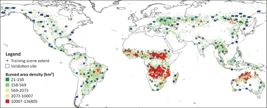
images. Main global burned area products include GBS (Carmona-Moreno et al., 2005), Global Burned
Area 2000 (GBA2000) (Tansey, 2004), GLOBSCAR (Simon, 2004), GlobCarbon (Plummer et al., 2006),
L3JRC (Tansey et al., 2008), MCD45 (Roy et al., 2005), GFED (Giglio et al., 2010), MCD64 (Giglio et al.,
2016), and Fire cci (Chuvieco et al., 2016).
   The recently released Fire cci product is produced based on MODIS images and has the highest spatial
resolution (250m) of all the existing global burned area products (Chuvieco et al., 2016; Pettinari and
Chuvieco, 2018). However, the requisites of the climate modelling community are not yet met with the
current global burned area products, as these products do not provide enough spatial detail (Bastarrika
et al., 2011). Imagery collected by the family of Landsat sensors is useful and appropriate for monitoring
the extent of area burned and provide spatial and temporal resolutions ideal for science and management
applications. Landsat sensors can provide a longer temporal record (from 1970s until now) of burned area
relative to existing global burned area products and potentially with increased accuracy and spatial detail
in most areas on the earth (Stroppiana et al., 2012). Great importance has been attached to developing
burned area products based on Landsat data in the past 10 years (Bastarrika et al., 2011; Stroppiana et al.,
2012; Hawbaker et al., 2017a). Up to now, there is no Landsat based global burned area product, however,
some regional Landsat burned area products have been publicly released in recent years. Australia released
its Fire Scars (AFS) products derived from all available Landsat 5, 7 and 8 images using time series change
detection technique (Goodwin and Collett, 2014). Fire scars are automatically detected and mapped using
dense time series of Landsat imagery acquired over the period 1987 2015 and the AFS product only covers
the state of Queensland, Australia. Monitoring Trends in Burn Severity (MTBS) project, sponsored by
the Wildland Fire Leadership Council (WFLC) provides consistent, 30-meter resolution burn severity data
and fire perimeters across all lands of the United States from 1984-2015 (only fires larger than 200 ha in
the eastern US and 400 ha in the western US are mapped) (Eidenshink et al., 2007). MTBS products are
generated based on the difference of Normalized Burned Ratio (NBR) calculated from pre-fire and post-
fire images, in which the burned area boundary is delineated by on-screen interpretation and the process
of developing a categorical burn severity product is subjective and dependent on analyst interpretation.
The Burned Area Essential Climate Variable (BAECV), developed by the U.S. Geological Survey (USGS),
produced Landsat derived burned area products across the conterminous United States (CONUS) from
1984-2015, and its products have been released in April 2017 (Hawbaker et al., 2017a). The main differences
between the MTBS and BAECV is the BAECV products are automatically generated based on all available
Landsat images.
   In summary, global burned area products are only available at coarse spatial resolution while 30-meter
resolution burned area products are limited to specific regions. The majority of coarse spatial resolution algo-
rithms developed to produce global burned area products use a multi-temporal change detection technique,
because such satellite data have very high temporal resolution and are capable of monitoring fire-affected
                                                       2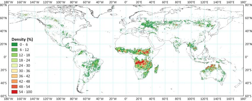
land cover changes. For example, the algorithm of MODIS burned area product (MCD45) is developed
from the bi-directional reflectance model-based expectation change detection approach (Roy et al., 2005).
One of the difficulties to produce Landsat based burned area products is that the traditional approaches
successfully applied to extract global burned area from MODIS, VEGETATION, etc. dont work well due
to the limited temporal resolution of the Landsat sensors. Moreover, the analysis of post-fire reflectance
may be easily contaminated by clouds or weakened by quick vegetation recovery, particularly in Tropical
regions (Alonso-Canas and Chuvieco, 2015). Another difficulty is that global 30-meter resolution annual
burned areas mapping needs to utilize dense time-series Landsat images, and the required datasets can be
hundreds of thousands of Landsat scenes, resulting impractical processing time. Although some researches
have been addressed to detect burned area regionally from Landsat time series (Goodwin and Collett, 2014;
Hawbaker et al., 2017b; Liu et al., 2018), results of global-scale have not been reported. However, thanks to
Google Earth Engine (GEE), a new generation of cloud computing platforms with access to a huge catalog
of satellite imagery and global-scale analysis capabilities (Gorelick et al., 2017), it is now possible to perform
global-scale geospatial analysis efficiently without caring about pre-processing of satellite images. In this
study, we focus on an automated approach to generate global-scale high resolution burned area map using
dense time-series of Landsat images on GEE, and a novel 30-meter resolution global annual burned area
map of 2015 (GABAM 2015) is released.

2. Methodology

2.1. Sampling design

   The spectral characteristics of burned areas vary in complex ways for different ecosystems, fire regimes
and climatic conditions. In terms of guaranteeing the accuracy of global burned area map and also the
completeness of quality assessment, a stratified random sampling method(Padilla et al., 2015; Boschetti
et al., 2016; Padilla et al., 2017) was used to generate two sets of sites for classifier training and the
validation of GABAM 2015, respectively. The training and validation sites were chosen randomly based on
stratifications of both fire frequency and type of land cover.
   Firstly, the Earth’s Land Surface was partitioned based on the 14 land cover classes according to the
MCD12C1 product (Friedl and Sulla-Menashe, 2015) of 2012 using University of Maryland (UMD) scheme.
These types were then merged into 8 categories based on their similarities (Chuvieco et al., 2011), i.e.
Broadleaved Evergreen, Broadleaved Deciduous, Coniferous, Mixed forest, Shrub, Rangeland, Agriculture
and Others. Table 1 shows the reclassification rule from UMD land cover types to new classifications. As
“Others” category consists of the biomes less prone to fire, only other 7 land cover categories are considered
to create the geographic stratifications in this work.

                                                         3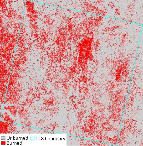
Table 1: Map between original UMD land cover types and new classifications for the geographic stratification.
New classification Original UMD type
Broadleaved Evergreen Evergreen Broadleaf forest
Broadleaved Deciduous Deciduous Broadleaf forest
Coniferous Evergreen Needleleaf forest
Deciduous Needleleaf forest
Mixed Forest Mixed forest
Shrub Closed shrublands
Open shrublands
Rangeland Woody savannas
Savannas
Grasslands
Agriculture Croplands
Others Water
Urban and built-up
Barren or sparsely vegetated
Secondly, the globe was divided into 5 partitions based on the BA density in 2015 provided by the
Global Fire Emissions Database (GFED) version 4.0 (Giglio et al., 2013), the most widely used inventory in
global biogeochemical and atmospheric modeling studies (Giglio et al., 2016). Specifically, GFED4 monthly
products of 2015 were utilized to produce an annual composition (GFED4 2015), consisting of 720 rows and
1440 columns which correspond to the global 0.25◦ × 0.25◦ GFED grid, and each pixel summed the total
areas of BA (BA density, km2 ) occurred in the grid cell during the whole year. The BA density of GFED4
2015 was then divided into 5 equal-frequency intervals (Chuvieco et al., 2011) with Quantile classification.
By spatially intersecting the 7 land cover categories and 5 BA density levels, we obtained the final 35
strata with different fire frequencies and biomes. The samples were equally allocated to 5 BA density levels,
but for different land cover categories, we also took into account the BA extent within each stratum with
larger sample sizes allocated to strata with higher BA extent (Padilla et al., 2014). According to the strategy
of stratified sampling, 120 samples (24 for each BA density level) were randomly selected to generate training
dataset, and spatial dimension of sampling units was based on Landsat World Reference System II (WRS-
II). Similarly, 80 validation sites (16 for each BA density level) were also created by randomly stratified
sampling, but trying to keep a distance (at least 200km) from the training samples so as not to fall into
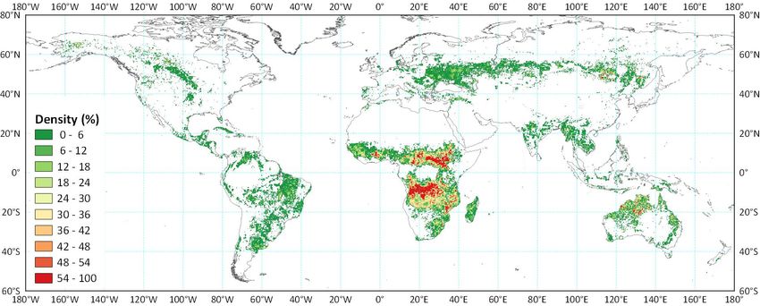
the extent of training Landsat scenes. Figure 1 illustrates the distribution of 120 random Landsat image
scenes and 80 validation sites over a map of BA density extracted from GFED4 2015, and Table 2 shows
4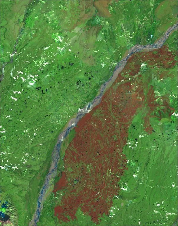
the distribution of training and validation samples over the different land cover types.

Figure 1: The distribution of 120 random Landsat image scenes and 80 validation sites over a map of BA density
extracted from GFED4 2015.

           Table 2: Distribution of training and validation samples over the different land cover types.
                Land cover type             Training sample count       Validation sample count
                Broadleaved Evergreen                  16                           11
                Broadleaved Deciduous                  12                           9
                Coniferous                             13                           9
                Mixed Forest                           12                           8
                Shrub                                  18                           12
                Rangeland                              25                           15
                Agriculture                            24                           16

2.2. Training dataset

   In terms of analyzing the characteristics of burned areas in Landsat images, 120 Landsat-8 image scenes
were chosen according to the WRS-II frames generated by stratified random sampling in section 2.1. All
the Landsat-8 images used in this study were acquired from datasets of USGS Landsat-8 Surface Re-
flectance Tier 1 and Tier 2 in Google Earth Engine platform, whose ImageCollection IDs are “LAND-
SAT/LC08/C01/T1 SR” and “LANDSAT/LC08/C01/T2 SR”. These data have been atmospherically cor-
rected using LaSRC (Vermote et al., 2016), and include a cloud, shadow, water and snow mask produced
using Fmask (Zhu and Woodcock, 2014), as well as a per-pixel saturation mask. For the purpose of burned
area mapping, 6 bands of Landsat-8 image were used, i.e. three Visible bands (BLUE, 0.452-0.512 µm;

                                                        5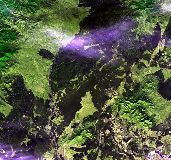
GREEN, 0.533-0.590 µm; RED, 0.636-0.673 µm), Near Infrared band (NIR, 0.851-0.879 µm), and two Short
Wave Infrared bands (SWIR1, 1.566-1.651 µm; SWIR2, 2.107-2.294 µm).
   In this work, burned area mapping algorithm was implemented on GEE platform, and the maximum
quantity of input samples are limited by GEEs classifiers, thus average 90–100 sample points were collected
by experienced experts from each Landsat-8 image, making the total quantity of sample points 12881 (6735
burned samples and 6146 unburned samples). Specifically, shortwave infrared (SWIR2), Near Infrared (NIR)
and Green bands were composited in a Red, Green, Blue (RGB) combination in order to visualize burned
areas better, and burned samples, including fire scars of different burn severity and of various biomass
types, were extracted from the pixels showing magenta color (Koutsias and Karteris, 2000). The unburned
pixels were extracted randomly over the non fire affected areas covering vegetation, built-up land, bare
land, topographic shadows, borders of lakes, etc. For those confusing pixels which were difficult to identify
whether they were burned scars, further check was performed by examining the Landsat images on nearest
date of the previous year or higher resolution images on nearest date in Google Earth software. To ensure
only clearly burned pixels were selected, the burned samples were collected carefully to avoid pixels near the
boundaries of burned scar (Bastarrika et al., 2011); and burned pixels located in burning flame or covered by
smoke were also excluded to prevent potential contamination of burned samples. Land surface reflectance
of the collected samples in BLUE, GREEN, RED, NIR, SWIR1, SWIR2 bands were extracted for further
analysis.

2.3. Sensitive features for burned surfaces
   Figure 2 shows the statistical mean reflectance (with standard deviations) of burned samples in Landsat
8 bands.

Figure 2: Means and standard deviations of land surface reflectance of burned Landsat-8 pixels in different bands.

   Burned areas are characterized by deposits of charcoal, ash and fuel, and the reflectance of the burned
                                                        6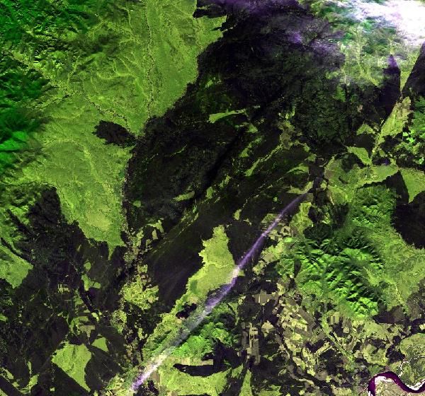
pixels generally increases along with the wave length while the burned pixels have similar reflectance in
SWIR1 and SWIR2 bands, which is greater than that in other bands. However, the spectral character of
post-fire pixels varies greatly (standard deviations in Figure 2) according to the type and condition of the
vegetation prior to burning and the degree of combustion (Bastarrika et al., 2014), and none of existing
spectral indices can be considered the best choice for identifying burned surfaces without misclassification
with other targets in all environments or fire regimes (Boschetti et al., 2010). Consequently, in this work, we
made use of most common spectral indices for Landsat image previously suggested in BA studies, and their
formulas are summarized as Table 3. Some of these spectral indices were specifically developed for burn
detection as they are sensitive to charcoal and ash deposition, such as normalized burned ratio (NBR (Key
and Benson, 1999)), normalized burned ratio 2 (NBR2 (Lutes et al., 2006)), burned area index (BAI (Martı́n,
1998)), mid infrared burn index (MIRBI (S. Trigg, 2001)). In addition, other indices that are not burn-
specific may also be useful to map burned areas when cooperating with burn-specific indices. For instance,
although normalized difference vegetation index (NDVI) is not the best index for burned area mapping,
it is sensitive to vegetation greenness and therefore to the absence of vegetation in the case of burned
areas (Stroppiana et al., 2009). The global environmental monitoring index (GEMI (Pinty and Verstraete,
1992)) is an improved vegetation index, specifically designed to minimize problems of contamination of the
vegetation signal by extraneous factors, and it is considered very important for the remote sensing of dark
surfaces, such as recently burned areas (Pereira, 1999). The soil adjusted vegetation index (SAVI (Huete,
1988)), which is originally designed for sparse vegetation and outperforms NDVI in environments with a
single vegetation (Veraverbeke et al., 2012), is also helpful to improve separability of burns from soil and
water (Stroppiana et al., 2012). The normalized difference moisture index (NDMI (Wilson and Sader,
2002)), which is sensitive to the moisture levels in vegetation, is also relative to fuel levels in fire-prone
areas. We also evaluated the relative importance of 14 Landsat features (8 spectral indices in Table 3 and
the surface reflectance in 6 bands of Landsat-8 image) when applied to classify burned areas using random
forest algorithm (Pedregosa et al., 2011) (as shown in Figure 3).
   Figure 3 shows that spectral indices were generally more important than the surface reflectance in most
bands, except for NIR band and SWIR2 band, which are sensitive to removal of vegetation cover and deposits
of char and ash (Pleniou and Koutsias, 2013). We also found that NBR2, BAI, MIRBI and SAVI had the
greatest relative importance, whereas SAVI was not initially developed for burned area detection. However,
considering the potential contribution of those features with relative low importance in distinguishing burned
scars, all of 14 features were selected as sensitive features to perform global burned area mapping in this
study.

                                                      7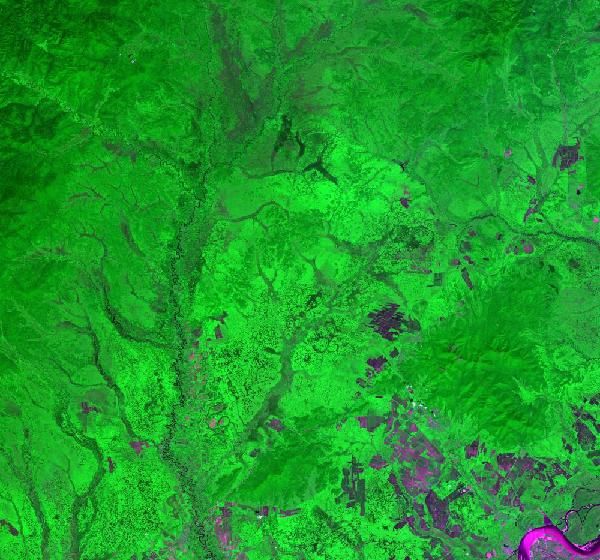
Table 3: The formulas of spectral indices that are sensitive to burned areas.
Name Formula
ρN IR −ρSW IR2
Normalized burned ratio N BR = ρN IR +ρSW IR2
IR1 −ρSW IR2
Normalized burned ratio 2 N BR2 = ρρSW
SW IR1 +ρSW IR2
1
Burned area index BAI = (ρN IR −0.06)2 +(ρRED −0.1)2
Mid infrared burn index M IRBI = 10ρSW IR2 − 0.98ρSW IR1 + 2
ρN IR −ρRED
Normalized difference vegetation index N DV I = ρN IR +ρRED
RED −0.125)
Global environmental monitoring index GEM I = η(1−0.25η)−(ρ1−ρRED ,
2(ρ2N IR −ρ2RED )+1.5ρN IR +0.5ρRED
η= ρN IR +ρRED +0.5
(1+L)(ρN IR −ρRED )
Soil adjusted vegetation index SAV I = ρN IR +ρRED +L , L = 0.5
IR −ρSW IR1
Normalized difference moisture index N DM I = ρρN N IR +ρSW IR1
ρRED is the surface reflectance in RED, ρN IR is the surface reflectance in NIR, ρSW IR1
is the surface reflectance in SWIR1 band, and ρSW IR2 is the surface reflectance in
SWIR2 band.
Ϭ͘ϮϬ
Ϭ͘ϭϱ
/ŵƉŽƌƚĂŶĐĞ
Ϭ͘ϭϬ
Ϭ͘Ϭϱ
Ϭ͘ϬϬ
>h
'Z
E Z
E/Z ^t/Zϭ ^t/ZϮ EZ EZϮ / '
D/ D/Z/ Es/ ^s/ ED/
Figure 3: Relative importance of Landsat image features on burned areas classification evaluated by random forest
algorithm.
2.4. Burned area mapping via GEE
In this work, annual burned area map is defined as spatial extent of fires that occurs within a whole year
and not of fires that occurred in previous years. Therefore, global 30-meter resolution annual burned areas
mapping needs to utilize dense time-series Landsat images, and the pipeline of annual burned area mapping
via GEE is described as Figure 4.
As shown in Figure 4, the pipeline mainly consists of three steps, model training, per-pixel processing
and burned area shaping, and the following provides more details of each step.
8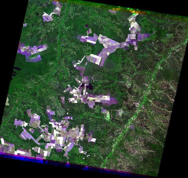
Per-pixel Processing
  MODIS VCF Product                                                         Tree
                                      Max Vegetation
    (Two years)                                                           Domination
                                                                                                          Seeds Filters
  Annual Landsat LSR                                                          Min NBR                      NDVI Filter
       Collection
    (Previous year)
                            Reflectance         Stack of
                                                                              Max NDVI                     NBR Filter
                               Stack           NDVI, NBR
                 QA
                Mask                                                           NDVI
                                                 Stack of                                               Temporal Filter
                            Reflectance
                                               Probability,
                               Stack
                                               NDVI, NBR                        NBR
  Annual Landsat LSR                                                                                    Probability Filter
      Collection
     (This year)
                                           Random Decision                   Max
                                                                          Probability                      Candidate
                                               Forests
                                                                                                            Seeds

                                                                                                            Merge
                                  Sensitive Features                                                    Connected Seeds

                            NBR         NBR2           BAI                         Per-pixel Burned      Remove Small
                                                                   Random            Probability          Components
   Global Training
                                                                    Forest
       Data                GEMI        MIRBI        NDVI
                                                                   Training
                                                                                                        Region Growing
                                                   SR of 6
                            SAVI        NDMI
                                                   bands                          Burned Area Shaping
                                                              Model Training
                                                                                                      Annual Burned
                                                                                                        Area Map
                 Figure 4: Workflow for annual burned area mapping using Google Earth Engine.

2.4.1. Model Training
   The random forest (RF) algorithm provided by GEE were applied to train a decision forest classifier,
and the global training data consisted of 6735 burned and 6146 unburned samples which were manually
collected from 120 Landsat scenes generated by stratified random sampling (in section 2.1 and section 2.2).
Random forest classifier with higher number of decision trees usually provides better results, but also causes
higher cost in computation time. Since the input features of the algorithm includes the surface reflectance
(SR) in 6 bands of Landsat-8 image as well as 8 spectral indices that have high sensitivity to burned surface,
we limited the number of decision trees in the forest to 100 for trade-off between accuracy and efficiency.
Additionally, we chose “probability” mode for GEE’s RF algorithm, in which the output is the probability
that the classification is correct, and the probability would be further utilized to perform region growing in
the step of burned area shaping.

                                                               9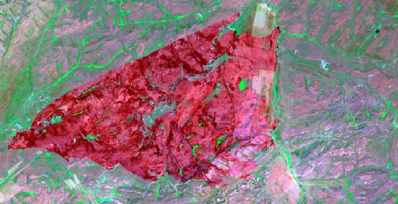
2.4.2. Per-pixel Processing
   In this step, Landsat surface reflectance collections from GEE, which consist of all the available Landsat
scenes, were employed for dense time-series processing. At a pixel, the occurrence of a single Landsat
satellite could be more than 20 or 40 times (considering the overlap between adjacent paths) within a
year, and it would double when contemporary satellites (e.g. Landsat-7 and Landsat-8) were utilized.
However, considering the failure of Scan Line Corrector (SLC) in the ETM+ instrument of Landsat-7
satellite, we only utilized USGS Landsat-8 Surface Reflectance collections (“LANDSAT/LC08/C01/T1 SR”
and “LANDSAT/LC08/C01/T2 SR”). The quality assessment (QA) band of Landsat image, which was
generated by FMask algorithm (Zhu and Woodcock, 2014), was used to perform QA masking. Pixels flagged
as being clouds, cloud shadows, water, snow, ice, or filled/dropped pixels were excluded from Landsat scenes,
and only clear land pixels remained after QA masking. At each pixel, the geometrically aligned dense time-
series Landsat image scenes provided a reflectance stack of 6 bands, which was then split into two stacks by
date filters, i.e. a stack of current year and that of the previous year.
   For the reflectance stack of current year, 8 spectral indices were computed at each time period, and
then the trained decision forest classifier in section 2.4.1 produced a stack of burned probability using the
8 spectral indices and the reflectance of 6 bands. The maximum value of a probability stack indicates the
probability that the pixel had ever appeared like burned scar during the whole year. Four quantities were
noted for each pixel, i.e. the date on which the maximum probability was observed (t1 ), as well as the
burned probability (pmax ), NDVI value (N DV I1 ) and NBR value (N BR1 ) on that date. However, it is not
usually possible to unambiguously separate in a single image the spectral signature of burned areas from
those caused by unrelated phenomena and disturbances such as shadows, flooding, snow melt, or agricultural
harvesting (Boschetti et al., 2015); the burned scars which occurred in previous years but not yet recovered
(particularly in boreal forests) should also be excluded from the annual BA map of current year. In this
sense, we also concerned the summary statistics of current year and previous year: N DV I2 , the maximum
NDVI value within the couple of years (current year and previous year); t2 , the date of N DV I2 ; and N BR2 ,
the minimum NBR value within the previous year. Then most of the unreasonable tree-covered burned-like
pixels would be excluded unless they met all the following constraints.

  1. N DV I2 > TN DV I , the maximum NDVI value within the couple of years should be greater than a
      threshold TN DV I . We choose NDVI as it has been found to be a good identifier of vigorous vegetation,
      and this constraint is used to exclude areas that appear like burned but in fact were just lacking
      vegetation.
  2. N DV I2 − N DV I1 > TdN DV I , the difference between the maximum NDVI and the NDVI when the
      pixel was most like burned scar should be greater than a threshold TdN DV I . This constraint ensures
      an evidence of vegetation decrease when burn happened.

                                                       10
3. N BR2 − N BR1 > TdN BR , the NBR value of a burned pixel should be less than the minimum NBR
of the previous year, and the threshold TdN BR is the minimum acceptable decline of NBR. This
constraint is useful to exclude false detections with periodic variation of NBR and NDVI, such as
mountain shadows, burned-like soil in deciduous season, snow melting and flooding.
4. t1 > t2 or t2 − t1 > TDAY , the most flourishing date of vegetation should be earlier than the burning
date, or the lagged days should be less than a threshold TDAY . For tree-covered surface, it usually
takes a long time for the vegetation to recover more flourishing than the previous year, thus the burn-
like pixels with t1ephemeral water or dark soils (Stroppiana et al., 2012)), and accepting all positive evidence can lead to
confusion errors. Although candidate seeds were chosen with high confidence, false seed pixels were still
frequently included in confusing surfaces, e.g. shadows, borders of lakes. Different from the candidate seeds
in the actual burned scars, those falsely introduced seed pixels always distributed sparsely. Consequently,
we aggregated the seed pixels into connected components using a kernel of 8-connected neighbors, and by
ignoring small fires with areas less than 1 ha (Laris, 2005), those fragmentary components (smaller than
11 pixels), which included most false seed pixels, were removed. Finally, an iterative procedure of region
growing were performed around each seed pixel. For each iteration, the 8-connected neighbors of the seed
pixels were aggregated as burned pixels (new seeds) if their burned probabilities were greater than or equal
to 0.5, and the iteration stopped when no more pixels can be aggregated as burned pixels. Figure 5 shows an
example of region growing. One can see that only some pixels showing strong magenta color in the burned
scars were chosen as seeds while those showing light magenta color were labeled as candidates for region
growing, including some actual burned pixels as well as some false detections (right-middle in Figure 5b).
However, after the processes of small seeds removal and region growing, the false detections were excluded
while those candidates near the seeds were aggregated to the final BA map.
3. Results and analysis
3.1. Product description
Employing the proposed approach, we produced the global annual burned area map of 2015 (GABAM
2015), which was projected in a Geographic (Lat/Long) projection at 0.00025◦ (approximately 30 me-
ters) resolution, with the WGS84 horizontal datum and the EGM96 vertical datum. The result consists
of 10x10 degree tiles spanning the range 180W180E and 80N60S and can be freely downloaded from
https://vapd.gitlab.io/post/gabam2015/. To make visualization of GABAM better, burned area density
is used instead of directly drawing the burned pixels on a global map, and it is defined as the proportion
of burned pixels in a 0.25◦ × 0.25◦ grid. An overview of global distribution of burned area density, derived
from the 1 arc-second resolution GABAM 2015, is shown in Figure 8a, together with that of the Fire cci
product in section 3.2.
Figure 6 illustrates an examples of GABAM 2015 in Canada, and the annually composited Landsat
reference images with minimum NBR values of 2015 and 2014 are also included. This region is located in
high latitude zones, and the burned scars may not completely recover within a year. Consequently, when
new burning occurs around the unrecovered burned scars, we must determine which burned scars come from
this year. Owing to the temporal filters, GABAM succeeded to clear up such confusion. From Figure 6b,
one can see that the burned scars mainly consist of two components, separated by the river. Figure 6a,
12(a) (b)
(c) (d)
Figure 5: Example of region growing for burned area detection. 5a is the Landsat-8 image displayed in false color
composition (red: SWIR2 band, green: NIR band and blue: GREEN band), 5b is the map of burned probability
generated by proposed method, 5c is the candidate seeds of burned area, 5d shows the final burned area map after
region growing.
however, shows that burned scars on the right side of the river can be observed in 2014, hence the result of
GABAM 2015 only remains the component on the left side.
3.2. Comparison with Fire cci product
3.2.1. Data preparing
As 30m resolution global burned area products are currently not available, we made a comparison between
GABAM 2015 and the Fire cci version 5.0 products (spatial resolution is approximately 250 meters) (Pet-
tinari and Chuvieco, 2018), which are based on MODIS on board the Terra satellite. The monthly Fire cci
pixel BA products of 2015 were composited as an annual pixel BA product by labeling the pixels as burned
ones once their values in Julian Day (the Date of the first detection) layer were valid (from 1 to 366) in
any of the 12 monthly products. Additionally, in order to perform regression analysis between two products
of different spatial resolution, we also produced an annual grid composition of BA within 2015 from the
composited annual pixel BA product by computing the proportion of burned pixels in each 0.25◦ × 0.25◦
grid. Note that the monthly grid BA products of Fire cci were not used to composite the annual grid prod-
13(a) 2014 (b) 2015 (c) BA
Figure 6: Burned area map example in Canada. 6a is the annually composited Landsat images of 2014 with the
minimum NBR values; 6b is the annually composited Landsat images of 2015; 6c shows the detected burned scars
occurred in 2015.
uct, because summing up the areas of BA for each grid in all monthly products might result in repetitive
counting at those pixels burned more than once within the year.
3.2.2. Visually comparing
Figure 7 shows an example of the two annual pixel BA products, and it can be seen that both products
correctly detected the BAs in Landsat image (Figure 7b), yet the BAs in Figure 7c occupy more pixels
than those in Figure 7d. Due to the limitation in spatial resolution of the input sensor of the Fire cci BA
product, some of the mixed pixels (consisting of burned and unburned pixels) may be classified as burned
ones. On the other hand, the result of GABAM 2015 shows finer boundaries of BAs, compared with that
of the Fire cci product.
3.2.3. Global grid map
Figure 8 illustrates the GABAM and Fire cci annual grid composition of BA, consisting of percentage
of burned pixels in each 0.25◦ × 0.25◦ grid. Figure 8b and Figure 8a show similar global distributions of BA
density.
3.2.4. Regression analysis
Figure 9 shows the proportion of BA in 0.25◦ × 0.25◦ grids of different land cover categories in Table 1,
for Fire cci product (x-axis) and GABAM 2015 (y-axis), and regression analysis was also performed between
the two products, providing a regression line (expressed as the slope and the intercept coefficient estimates)
14(a) (b)
(c) (d)
Figure 7: Comparison between Fire cci and GABAM. 7a and 7b are the Landsat-8 images before (June 24th, 2015)
and after (July 26th, 2015) fire, respectively, displayed in false color composition (red: SWIR2 band, green: NIR
band and blue: GREEN band); 7c shows the burned areas of annually composited Fire cci product, and 7d shows
the burned areas generated by proposed method.
and the coefficient of determination (R2 ) for each land cover category (Figure 9a–9h) and for global scale
(Figure 9i). Moreover, as many points overlapped in the scatter graphs, we also rendered the scatters with
different colors according to the number of grid cells (1 to 10 or more) having the same proportion values.
According to Figure 9, the intercept values of the estimated regression lines were close to 0 while the slopes
were lower than 1, showing that GABAM 2015 generally underestimated (Chuvieco et al., 2011) burned scars
compared with Fire cci product. Moreover, the distribution and color of scatters in Figure 9i also show that
15(a) GABAM 2015
(b) Fire cci 2015
Figure 8: Global distribution of burned area density (percentage of burned pixels in every 0.25◦ × 0.25◦ grid) of
GABAM and Fire cci product within 2015. 8a is the annual grid composition of BA of GABAM, and 8b is that of
the Fire cci product.
a large number of grids were considered to have higher burned proportion by Fire cci product than by
GABAM. The main reason for the inconsistence can be attributed to the difference in spatial resolution of
data sources, and less pixels were commonly classified as BA in Landsat images, e.g. Figure 7. Specifically,
only a few 0.25◦ × 0.25◦ grids were occupied by more than 90% BA in GABAM while grids with high
proportion of BA were more common in Fire cci product.
Considering the coefficients of determination of estimated regression lines, the two products showed
highest linear relationship strengths in coniferous forest (R2 = 0.82), rangeland (R2 = 0.75) and shrub
16Broadleaved Evergreen Broadleaved Deciduous Coniferous
y = 0.59x + 0.36, R2 = 0.45 y = 0.48x + 0.18, R2 = 0.38 y = 0.64x + 0.03, R2 = 0.82
10 10 10
70
Burned proportion from GABAM (%)
Burned proportion from GABAM (%)
Burned proportion from GABAM (%)
9 35 9 9
80
60 8 30 8 8
50 7 25 7 7
60
6 20 6 6
40
5 5 40 5
30 15
4 4 4
20 10
3 3 20 3
10 5
2 2 2
0
0 0
1 1 1
0 20 40 60 0 10 20 30 0 20 40 60 80
Burned proportion from Fire cci (%) Burned proportion from Fire cci (%) Burned proportion from Fire cci (%)
(a) (b) (c)
Shrub Rangeland Agriculture
y = 0.76x + 0.25, R2 = 0.62 y = 0.84x + 1.02, R2 = 0.75 y = 0.54x + 1.25, R2 = 0.31
10 100 10 10
Burned proportion from GABAM (%)
Burned proportion from GABAM (%)
9 9
Burned proportion from GABAM (%)
9
80
80
8 80 8
8
7 7 7
60 60
60
6 6 6
5 5 40 5
40 40
4 4 4
20 3 20 3 20 3
2 2 2
0 1 0 1
0 1
0 20 40 60 80 0 20 40 60 80 100 0 20 40 60 80
Burned proportion from Fire cci (%) Burned proportion from Fire cci (%) Burned proportion from Fire cci (%)
(d) (e) (f)
Mixed Forest Others
Global
y = 0.57x + 0.18, R2 = 0.45 y = 0.51x + 0.03, R2 = 0.07
10 8 y = 0.83x + 0.14, R2 = 0.74
80 100 10
35
Burned proportion from GABAM (%)
Burned proportion from GABAM (%)
9
Burned proportion from GABAM (%)
7 9
70
30
8 80
8
60 6
7 25
7
50 60
20 5
6 6
40
5 15 4 5
40
30
4 4
10 3
20
3 20 3
5
10 2
2 2
0
0 1 0
1 1
0 20 40 60 80 0 10 20 30 0 20 40 60 80 100
Burned proportion from Fire cci (%) Burned proportion from Fire cci (%) Burned proportion from Fire cci (%)
(g) (h) (i)
Figure 9: Scatter graphs and regression lines between GABAM and Fire cci. 9a–9h are the results in different land
cover categories; 9i shows the global result in all kinds of land covers. The color scheme illustrates the number of
grid cells having the same proportion values.
17(R2 = 0.62), and lowest strengths in agriculture land (R2 = 0.31) and “Others” category (R2 = 0.07).
In “Others” category, which is considered to be not prone to fire, the two products only included a few
grids containing BA (with low burned proportions), thus they were not likely to be correlated; the low
correlation in agriculture land is owing to the uncertainty of both products, which will be further discussed
in section 3.4.
The quantity and color of scatters in Figure 9 indicate that most of burned areas were located in range-
land, and the global relationship (Figure 9i) of the GABAM and Fire cci product was mainly determined
by that in rangeland (Figure 9e), i.e. woody savannas, savannas and grasslands.
3.3. Validation
3.3.1. Data sources
Accuracy assessment was carried out according to the 80 validation sites which were created in section 2.1,
and the reference data were selected in these sites from multiple data sources, including fire perimeter
datasets and satellite images. Commonly, when satellite data are used as reference data, they should have
higher spatial resolution than the data used to generate the BA product (Boschetti et al., 2009). For Landsat
BA product, however, access to global higher-resolution time-series satellite data is difficult, and a thorough
validation of Landsat science products can be completed with independent Landsat-derived reference data
while strengthened by the use of complementary sources of high-resolution data (Vanderhoof et al., 2017).
Consequently, in this study, some publicly available satellite images of higher-resolution were included in the
validation scheme, while Landsat was the majority of validation data source. Specifically, Landsat-8 (LC8)
images were employed to generate reference data independently for most of the validation sites except those
located in the United States (U.S.), South America and China. In U.S., MTBS perimeters of 2015 were used
as the supplemental reference data of LC8 images, and in South America and China, CBERS-4 MUX (CB4)
and Gaofen-1 WFV (GF1) satellite images were used to create perimeters of burned area, respectively. The
characteristics of CB4 and GF1 are illustrated in Table 4. Note that the size of validation site varied by
the type of data source, i.e. a WRS-II frame (about 185km × 185km) for Landsat images, a scene for CB4
images (about 120km × 120km) and a box of 100km × 100km for GF1 images. Using Landsat frames
or image scenes as a unit of validation site is convenient for data downloading and processing; we chose a
smaller box for GF1 to improve the data availability considering the extents of GF1 frames or scenes are
not fixed due to the long orbital return period.
18Table 4: Characteristics of CBERS-4 MUX and Gaofen-1 WFV.
Spatial resolution Swath width Spectral bands (µm)
Sensors
at nadir (m) at nadir (km) blue green red NIR
CBERS-4 MUX 20 120
0.45-0.52 0.52-0.59 0.63-0.69 0.77-0.89
Gaofen-1 WFV 16 192
3.3.2. Reference data generation
In each validation site, all the available image scenes (LC81 , CB42 or GF13 ) acquired in 2015 were used.
LC8 images were ortho-rectified surface reflectance products, CB4 images were ortho products, and GF1
images were not geometrically rectified. The procedure of generating reference BA can be summarized as
following steps.
1. Preprocessing
All the images utilized to generate BA reference data were spatially aligned with mean squared error
less than 1 pixel. The ortho-rectified LC8 and CB4 images met the requirement of geometric accuracy,
yet the GF1 images did not. Accordingly, an automated method (Long et al., 2016) was applied to
ortho-rectify the time-series GF1 images, taking the LC8 panchromatic images (spatial resolution is
15 meters) as geo-references.
2. BA Detection
BA perimeters were generated from the time-series images via a semi-automatic approach. Firstly,
image pairs (pre- and post-fire) were manually selected from the time-series image by checking whether
any new burned scars appeared in the newer images. For LC8 images, SWIR2, NIR and Green bands
were composited in a Red, Green, Blue (RGB) combination; for CB4 and GF1 images, Red, NIR and
Green bands were composited in an RGB combination. The identification of BA might be difficult
for CB4 and GF1 images due to the lack of shortwave infrared bands, thus Fire cci BA product was
used to verify the BA identification. Secondly, burned and unburned samples were manually collected
from each selected image pair. The burned samples included only the newly burned scars, which
appeared burned in the newer image but unburned in the older image; the unburned samples consisted
of unburned pixels, partially recovered BA pixels, and also pixels covered by cloud or cloud shadows
in either images. Afterwards, the support vector machines (SVM) classifier in ENVITM software were
used to classify each image pair into burned and unburned pixels, and the detected burned pixels in
all the image pairs were integrated to create a composited annual BA map. Note that the sensitive
1 https://earthexplorer.usgs.gov
2 http://www.dgi.inpe.br/catalogo/
3 http://218.247.138.119:7777/DSSPlatform/productSearch.html
19features in section 2.3 were utilized in SVM for each LC8 image pair; but for CB4 and GF1 images,
features used for classification consisted of the digital number (DN) values in four bands of an image
pair (totally 8 DN values), as most of the burned-sensitive spectral indices cannot be derived from the
RGB-NIR bands. Finally, the BA perimeters of 2015 were generated from the annual BA composition
using the vectorization tool in ArcGISTM software.
3. Reviewing and manually revision
The result of supervised classifier (SVM) and automated vectorization algorithm might not be perfect,
thus BA perimeters were further edited visually by experienced experts, via overlapping the vector
layer of BA perimeters with the satellite image layers.
Additionally, in U.S., MTBS perimeters of 2015 were directly used as the main reference data, supple-
mented by the interpreted results of LC8 time-series images, which could help to avoid missing of small
fires.
3.3.3. Validation results
To assess the accuracy of GABAM 2015, a cross tabulation (Pontius and Millones, 2011) between the
pixels assigned by in our BA product and in the reference data was computed to produce the confusion matrix
for each validation site. Afterwards, the global cross tabulation (Table 5) was generated by averaging all
the cross tabulations.
Table 5: Cross tabulation between GABAM 2015 and the reference data.
Reference data (pixel)
Burned Unburned Total
Burned 5473720 (X11 ) 823170 (X12 ) 6296890
GABAM 2015 (pixel) Unburned 2360096 (X21 ) 43661559 (X22 ) 46021655
Total 7833816 44484729 52318545
Finally, three statistics, i.e. commission error, omission error and overall accuracy, can be derived from
the confusion matrix:
• Commission Error (Ec ): X12 /(X11 +X12 ), the ratio between the false BA positives (detected burned
areas that were not in fact burned) and the total area classified as burned by GABAM 2015.
• Omission Error (Eo ): X21 /(X11 + X21 ), the ratio between the false BA negatives (actual burned
areas not detected) and the total area classified as burned by the reference data.
• Overall Accuracy (Ao ): (X11 + X12 )/(X11 + X12 + X21 + X22 ), the ratio between the area classified
correctly and the total area to evaluate.
20According to Table 5, Ec and Eo of GABAM 2015 were 13.17% and 30.13%, respectively, while Ao was
93.92%. Generally, GABAM 2015 was expected to have a lower Ec but a higher Eo . High omission error
might result from several reasons:
1. In the validation sites located in tropical zones, clear burned evidences were frequently missed by
Landsat sensor due to the quick recovery of the vegetation surface. This point will be further discussed
in section 3.4.
2. Some pixels located within a burned area, but not showing strong burned appearance, might be
excluded by GABAM 2015 (e.g. Figure 7d), while they were considered as a part of a complete burned
scar in the reference data. Particularly, high Eo was found in those validation sites using MTBS
perimeters, e.g. Ec and Eo of the validation site in Figure A.16 were 1.45% and 67.97%.
Table 6 shows the average accuracy of GABAM 2015 in various land cover categories, and more details
of validation can be found in appendix Appendix A, which includes 5 examples of validation sites from
various regions, with different data sources as reference data.
Table 6: Information of site validation examples.
Land cover type Ec (%) Eo (%) Ao (%)
Broadleaved Evergreen 8.64 10.95 90.99
Broadleaved Deciduous 23.59 34.85 99.03
Coniferous 7.41 18.27 99.77
Mixed Forest 8.73 34.33 98.36
Shrub 13.00 3.78 99.49
Rangeland 11.91 23.06 91.79
Agriculture 10.91 45.38 94.41
3.4. Discussion
Different from the satellite images of coarse spatial resolution, the temporal resolution of Landsat images
is not high enough to capture the short-term events on the earth. Specifically, the general revisit period of
Landsat image is more than 10 days, hence active fire will be observed by Landsat satellite with probability
less than 10% (considering the cloud coverage). In addition, the gaps between Landsat images of adjacent
time phases and the occurrence of cloud also increase the uncertainty to analyze the time-series patterns
of land surface. Without using the evidence of active fire, it is not easy to identify the burned scars at
global-scale with high confidence due to the wide variety of vegetation types, phenological characters and
burned-like landcovers, and spectral characteristics within a burned scar (char, scorched leaves or grass, or
21even green leaves when the fire is not very severe(Bastarrika et al., 2011)). In this work, MODIS Vegetation
Continuous Fields (VCF) product was applied to discriminate tree-dominated and grass-dominated regions,
but the VCF product is neither precise in spatial resolution nor available before 2000 year and, moreover,
two categories is far from enough to separate different burning types. Actually, much prior knowledge
can be utilized to improve the accuracy of GABAM, if the globe is carefully divided into intensive regions
according to the fire behaviour, land cover types and climate. For instance, most biomass burning in
the tropics is limited to a burning season, around 10% of the savanna biome burns every year, burning
cropland after a harvest is extremely prevalent, and so on. Consequently, region-specified algorithms should
be helpful to improve the accuracy of high-resolution global annual burned area mapping. Furthermore,
despite of the high correlation between GABAM and Fire cci, the area of detected BA was generally smaller
in GABAM than that in Fire cci, since some pixels located within a burned area but not showing strong
burned appearance, were not included in GABAM. This situation can be considered as underestimation of
BA or omission error if only taking into account the connectivity and completeness of burned patches; on
the other hand, however, the detailed perimeter of BA from GABAM can be useful to statistics the area of
biomes actually burned, and therefore to improve the simulation of carbon emissions from biomass burning.
At present form, however, GABAM suffers limitations in the following aspects.
3.4.1. BA in Agriculture land
It is difficult to detect BA in cropland with high confidence (low commission error and low omission
error) from satellite images:
• A lot of croplands have comparable spectral characteristics to burned areas when harvested or ploughed.
• The temporal behaviour of harvest or burning of cropland is similar to that of grassland fire, e.g.
sudden decline and gradual recovery of NDVI, and periodic variation of NBR values year after year.
• Different from the wildfires in rangeland and forest, most of the fires in croplands are human-intended
stubble burning, and they are commonly small and of short duration, difficult to be captured by
satellite sensors. In this sense, the traditional burned area detection algorithms, which are frequently
used to generate BA products from data source of the middle resolution (e.g. MODIS, AVHRR,
MERIS) are likely to have high omission error in croplands for small cropland fire.
Figure 10 shows an example of cropland in Mykolayiv, Ukraine, including the Landsat-8 time series
(Figure 10a–10j) and the burned scars mapped by Fire cci (Figure 10k) and GABAM (Figure 10l). Small
fire spots, showing light orange color, can be visually observed from Figure 10a, 10b and 10i, but burned
scars surrounding these fire spots were not included in Fire cci product. On the other hand, without fire
evidence or field validation, it is also difficult to tell whether the burned-like surfaces detected by GABAM
were false alarms.
22Due to these difficulties, discriminating true-burned areas from croplands is not a trivial task, and
cropland masks can be employed to remove potential confusions.
3.4.2. Omission of observations
Using Landsat images as input data for GABAM, the number of valid observations is a limiting factor
for detecting fires, since the active- or post-fire evidence may be omitted or weaken due to the temporal
gaps caused by temporal resolution as well as cloud contamination. Especially in Tropical regions, where
vegetation recovery is quite quick after fire, temporal gaps usually result in high omission error. Figure 11
shows an example of omission error in South America. From the CBERS-4 images (Figure 11p–11s), a new
burned scar, which occurred during August 21 to October 12, can be identified at the center of image patch.
However, all the Landsat-8 images (Figure 11a–11o) acquired between the date interval from September 21
to November 24 were contaminated by cloud, thus the region covering this burned scar in these images were
masked by QA band during the process of BA detecting.
3.4.3. Validation
For satellite data product validation, a commonly used method is to employ higher spatial resolution
satellite data. For example, in order to validate MODIS derived data product (1 km spatial resolution),
Landsat satellite data is commonly used. In this study, however, Landsat images were used as the main
reference source to validate Landsat derived burned area product. Although the validation process was
conducted by independent experienced experts with great caution, relying on Landsat for both product
generation and validation limits our ability to assess inaccuracies imposed by the satellite sensor itself, such
as radiometric calibration accuracy, spectral band settings, geolocation and mixed pixels (Strahler et al.,
2006). Accordingly, extensive validation of GABAM is expected to be further performed by professional
users.
4. Conclusions
An automated pipeline for generating 30m resolution global-scale annual burned area map utilizing
Google Earth Engine was proposed in this study. Different from the previous coarse resolution global
burned area products, GABAM 2015, a novel 30-m resolution global annual burned area map of 2015 year,
was derived from all available Landsat-8 images, and its commission error and omission error are 13.17%
and 30.13%, respectively, according to global validation. Comparison with Fire cci product showed a similar
spatial distribution and strong correlation between the burned areas from the two products, particularly
in coniferous forests. The automated pipeline makes it possible to efficiently generate GABAM from huge
catalog of Landsat images, and our future effort will be concentrated to produce long time-series 30m
resolution GABAMs.
23(a) 2015-02-17 (b) 2015-03-21 (c) 2015-05-24 (d) 2015-06-02
(e) 2015-06-09 (f) 2015-06-25 (g) 2015-09-22 (h) 2015-09-29
(i) 2015-10-15 (j) 2015-10-31 (k) BA from Fire cci (l) BA from GABAM
Figure 10: Burned area map example of croplands in Mykolayiv, Ukraine. 10a–10j shows the Landsat-8 images
displayed in false color composition (red: SWIR2 band, green: NIR band and blue: GREEN band); 10k and 10l
show the BA from Fire cci product and GABAM 2015, respectively.
24(a) 2015-05-16 (LC8) (b) 2015-06-01 (LC8) (c) 2015-06-17 (LC8) (d) 2015-07-03 (LC8)
(e) 2015-07-19 (LC8) (f) 2015-08-04 (LC8) (g) 2015-08-20 (LC8) (h) 2015-09-05 (LC8)
(i) 2015-09-21 (LC8) (j) 2015-10-07 (LC8) (k) 2015-10-23 (LC8) (l) 2015-11-08 (LC8)
(m) 2015-11-24 (LC8) (n) 2015-12-10 (LC8) (o) 2015-12-26 (LC8) (p) 2015-06-30 (CB4)
(q) 2015-07-26 (CB4) (r) 2015-08-21 (CB4) (s) 2015-10-12 (CB4) (t) Detected BA
Figure 11: Example of omission error of GABAM 2015. 11a–11o are Landsat-8 image patches displayed in false color
composition (red: SWIR2 band, green: NIR band and blue: GREEN band), 11p–11s are CBERS-4 image patches
displayed in false color composition (red: NIR band, green: RED band and blue: GREEN band), and 11t shows
the detected BA.
25Acknowledgments
This research has been supported by The National Key Research and Development Program of China
(2016YFA0600302 and 2016YFB0501502), and National Natural Science Foundation of China (61401461
and 61701495).
Appendix A. Examples of validation sites
Figure A.12–A.16 show some examples of site validation, and Table A.7 summarizes the information of
these validation sites, including the location, source of reference data, commission error, omission error and
overall accuracy.
Table A.7: Information of site validation examples.
ID Location Reference data Ec (%) Eo (%) Ao (%) Figure
1 China GF1 8.64 10.95 90.99 Figure A.12
2 South America CB4 13.95 33.25 94.88 Figure A.13
3 Africa LC8 41.23 57.41 71.29 Figure A.14
4 Australia LC8 0.77 20.88 90.22 Figure A.15
5 U.S. LC8 & MTBS 1.45 67.97 95.87 Figure A.16
26(a) 2015-04-01 (GF1) (b) 2015-05-03 (GF1) (c) 2015-05-20 (GF1)
(d) 2015-07-16 (GF1) (e) 2015-10-15 (GF1) (f) 2015-11-08 (GF1)
(g) 2015-11-20 (GF1) (h) BA (GF1) (i) Detected BA
Figure A.12: Example of validation using GF-1 images. A.12a–A.12g show the GF-1 images used to generate
reference map, displayed in false color composition (red: NIR band, green: RED band and blue: GREEN band),
A.12h is reference BA map generated from GF-1 images, and A.12i is detected BA by proposed method.
27(a) 2015-06-01 (CB4) (b) 2015-07-06 (CB4) (c) 2015-08-01 (CB4)
(d) 2015-08-27 (cb4) (e) 2015-09-22 (CB4) (f) 2015-11-18 (CB4)
(g) 2015-12-09 (CB4) (h) BA (CB4) (i) Detected BA
Figure A.13: Example of validation using CBERS-4 images. A.13a–A.13g show the CBERS-4 images used to generate
reference map, displayed in false color composition (red: NIR band, green: RED band and blue: GREEN band),
A.13h is reference BA map generated from CBERS-4 images, and A.13i is detected BA by proposed method.
28(a) 2014-12-19 (LC8) (b) 2015-01-04 (LC8) (c) 2015-01-20 (LC8) (d) 2015-02-05 (LC8)
(e) 2015-02-21 (LC8) (f) 2015-03-09 (LC8) (g) 2015-11-04 (LC8) (h) 2015-11-20 (LC8)
(i) 2015-12-06 (LC8) (j) 2015-12-22 (LC8) (k) BA (LC8) (l) Detected BA
Figure A.14: Example of validation using Landsat-8 images (path/row:193/054) in Africa. A.14a–A.14j show the
Landsat-8 images used to generate reference map, displayed in false color composition (red: SWIR2 band, green:
NIR band and blue: GREEN band), A.14k is reference BA map generated from Landsat-8 images, and A.14l is
detected BA by proposed method.
29(a) 2015-01-21 (LC8) (b) 2015-02-06 (LC8) (c) 2015-06-30 (LC8)
(d) 2015-10-20 (LC8) (e) 2015-11-21 (LC8) (f) 2015-12-23 (LC8)
(g) BA (LC8) (h) Detected BA
Figure A.15: Example of validation using Landsat-8 images (path/row:104/074) in Australia. A.14a–A.14j show the
Landsat-8 images used to generate reference map, displayed in false color composition (red: SWIR2 band, green:
NIR band and blue: GREEN band), A.14k is reference BA map generated from Landsat-8 images, and A.15h is
detected BA by proposed method.
30(a) 2015-06-25 (LC8) (b) 2015-09-29 (LC8)
(c) MTBS BA perimeters (d) Reference BA perimeters (e) Detected BA
Figure A.16: Comparison between MTBS and detected BA. A.16a and A.16b are the Landsat-8 images
(path/row:044/026) displayed in false color composition (red: SWIR2 band, green: NIR band and blue: GREEN
band), A.16c is the MTBS perimeters of 2015, A.16d shows reference BA perimeters generated from Landsat-8 images
and MTBS perimeters of 2015, and A.16e shows burned areas generated by proposed method.
Reference
References
Alonso-Canas, I., Chuvieco, E., 2015. Global burned area mapping from ENVISAT-MERIS and MODIS active fire data.
Remote Sensing of Environment 163, 140–152. URL: https://doi.org/10.1016%2Fj.rse.2015.03.011, doi:10.1016/j.rse.
2015.03.011.
Bastarrika, A., Alvarado, M., Artano, K., Martinez, M., Mesanza, A., Torre, L., Ramo, R., Chuvieco, E., 2014. BAMS: A tool
for supervised burned area mapping using landsat data. Remote Sensing 6, 12360–12380. URL: https://doi.org/10.3390%
2Frs61212360, doi:10.3390/rs61212360.
Bastarrika, A., Chuvieco, E., Martı́n, M.P., 2011. Mapping burned areas from landsat TM/ETM+ data with a two-phase
algorithm: Balancing omission and commission errors. Remote Sensing of Environment 115, 1003–1012. URL: https:
//doi.org/10.1016%2Fj.rse.2010.12.005, doi:10.1016/j.rse.2010.12.005.
31Boschetti, L., Roy, D., Justice, C., 2009. International global burned area satellite product validation protocol (part i–production
and standardization of validation reference data), in: CEOS-CalVal, (Ed.). USA: Committee on Earth Observation Satellites,
pp. 1–11.
Boschetti, L., Roy, D.P., Justice, C.O., Humber, M.L., 2015. MODIS–landsat fusion for large area 30m burned area mapping.
Remote Sensing of Environment 161, 27–42. URL: https://doi.org/10.1016%2Fj.rse.2015.01.022, doi:10.1016/j.rse.
2015.01.022.
Boschetti, L., Stehman, S.V., Roy, D.P., 2016. A stratified random sampling design in space and time for regional to global
scale burned area product validation. Remote Sensing of Environment 186, 465–478. URL: https://doi.org/10.1016%2Fj.
rse.2016.09.016, doi:10.1016/j.rse.2016.09.016.
Boschetti, M., Stroppiana, D., Brivio, P.A., 2010. Mapping burned areas in a mediterranean environment using soft integration
of spectral indices from high-resolution satellite images. Earth Interactions 14, 1–20. URL: https://doi.org/10.1175%
2F2010ei349.1, doi:10.1175/2010ei349.1.
Carmona-Moreno, C., Belward, A., Malingreau, J.P., Hartley, A., Garcia-Alegre, M., Antonovskiy, M., Buchshtaber, V.,
Pivovarov, V., 2005. Characterizing interannual variations in global fire calendar using data from earth observing satellites.
Global Change Biology 11, 1537–1555. URL: https://doi.org/10.1111%2Fj.1365-2486.2005.01003.x, doi:10.1111/j.
1365-2486.2005.01003.x.
Chuvieco, E., Padilla, M., Hantson, S., Theis, R., Snadow, C., 2011. Esa cci ecv fire disturbance-product validation plan (v3.
1). ESA Fire-CCI project (http://www. esa-fire-cci. org/) .
Chuvieco, E., Yue, C., Heil, A., Mouillot, F., Alonso-Canas, I., Padilla, M., Pereira, J.M., Oom, D., Tansey, K., 2016. A new
global burned area product for climate assessment of fire impacts. Global Ecology and Biogeography 25, 619–629. URL:
https://doi.org/10.1111%2Fgeb.12440, doi:10.1111/geb.12440.
DAAC, N.L., 2015. Modis vegetation continuous fields (vcf) product. version 5.1. https://lpdaac.usgs.gov/dataset_
discovery/modis/modis_products_table/mod44b. doi:10.4225/13/511C71F8612C3. nASA EOSDIS Land Processes DAAC,
USGS Earth Resources Observation and Science (EROS) Center, Sioux Falls, South Dakota (https://lpdaac.usgs.gov).
Eidenshink, J., Schwind, B., Brewer, K., Zhu, Z.L., Quayle, B., Howard, S., 2007. A project for monitoring trends in burn sever-
ity. Fire Ecology 3, 3–21. URL: https://doi.org/10.4996%2Ffireecology.0301003, doi:10.4996/fireecology.0301003.
Friedl, M., Sulla-Menashe, D., 2015. Mcd12c1 modis/terra+aqua land cover type yearly l3 global 0.05deg cmg. https:
//lpdaac.usgs.gov/dataset_discovery/modis/modis_products_table/mcd12c1. doi:10.5067/MODIS/MCD12C1.006. nASA
EOSDIS Land Processes DAAC (https://lpdaac.usgs.gov).
Giglio, L., Randerson, J.T., van der Werf, G.R., 2013. Analysis of daily, monthly, and annual burned area using the fourth-
generation global fire emissions database (GFED4). Journal of Geophysical Research: Biogeosciences 118, 317–328. URL:
https://doi.org/10.1002%2Fjgrg.20042, doi:10.1002/jgrg.20042.
Giglio, L., Randerson, J.T., van der Werf, G.R., Kasibhatla, P.S., Collatz, G.J., Morton, D.C., DeFries, R.S., 2010. Assessing
variability and long-term trends in burned area by merging multiple satellite fire products. Biogeosciences 7, 1171–1186.
URL: https://doi.org/10.5194%2Fbg-7-1171-2010, doi:10.5194/bg-7-1171-2010.
Giglio, L., Schroeder, W., Justice, C.O., 2016. The collection 6 MODIS active fire detection algorithm and fire products.
Remote Sensing of Environment 178, 31–41. URL: https://doi.org/10.1016%2Fj.rse.2016.02.054, doi:10.1016/j.rse.
2016.02.054.
Goodwin, N.R., Collett, L.J., 2014. Development of an automated method for mapping fire history captured in landsat
TM and ETM+ time series across queensland, australia. Remote Sensing of Environment 148, 206–221. URL: https:
//doi.org/10.1016%2Fj.rse.2014.03.021, doi:10.1016/j.rse.2014.03.021.
Gorelick, N., Hancher, M., Dixon, M., Ilyushchenko, S., Thau, D., Moore, R., 2017. Google earth engine: Planetary-scale
geospatial analysis for everyone. Remote Sensing of Environment 202, 18–27. URL: https://doi.org/10.1016%2Fj.rse.
32You can also read