SuperNet - An efficient method of neural networks ensembling - arXiv
←
→
Page content transcription
If your browser does not render page correctly, please read the page content below
SuperNet - An efficient method of neural
                                                            networks ensembling
                                                              Ludwik Bukowski∗+ and Witold Dzwinel†+
                                         +
                                             AGH University of Science and Technology, WIET, Department of
arXiv:2003.13021v1 [cs.LG] 29 Mar 2020

                                                          Computer Science, Kraków, Poland

                                                                                  March 31, 2020

                                                                                        Abstract
                                                        The main flaw of neural network ensembling is that it is exceptionally de-
                                                   manding computationally, especially, if the individual sub-models are large
                                                   neural networks, which must be trained separately. Having in mind that mod-
                                                   ern DNNs can be very accurate, they are already the huge ensembles of simple
                                                   classifiers, and that one can construct more thrifty compressed neural net of
                                                   a similar performance for any ensemble, the idea of designing the expensive
                                                   SuperNets can be questionable. The widespread belief that ensembling in-
                                                   creases the prediction time, makes it not attractive and can be the reason
                                                   that the main stream of ML research is directed towards developing better
                                                   loss functions and learning strategies for more advanced and efficient neural
                                                   networks. On the other hand, all these factors make the architectures more
                                                   complex what may lead to overfitting and high computational complexity, that
                                                   is, to the same flaws for which the highly parametrized SuperNets ensembles
                                                   are blamed. The goal of the master thesis is to speed up the execution time re-
                                                   quired for ensemble generation. Instead of training K inaccurate sub-models,
                                                   each of them can represent various phases of training (representing various
                                                   local minima of the loss function) of a single DNN [Huang et al., 2017; Gripov
                                                   et al., 2018]. Thus, the computational performance of the SuperNet can be
                                                   comparable to the maximum CPU time spent on training its single sub-model,
                                                   plus usually much shorter CPU time required for training the SuperNet cou-
                                                   pling factors.

                                         ∗
                                                 the Author of this thesis and corresponding author
                                             †
                                                 MsC thesis supervisor

                                                                                            i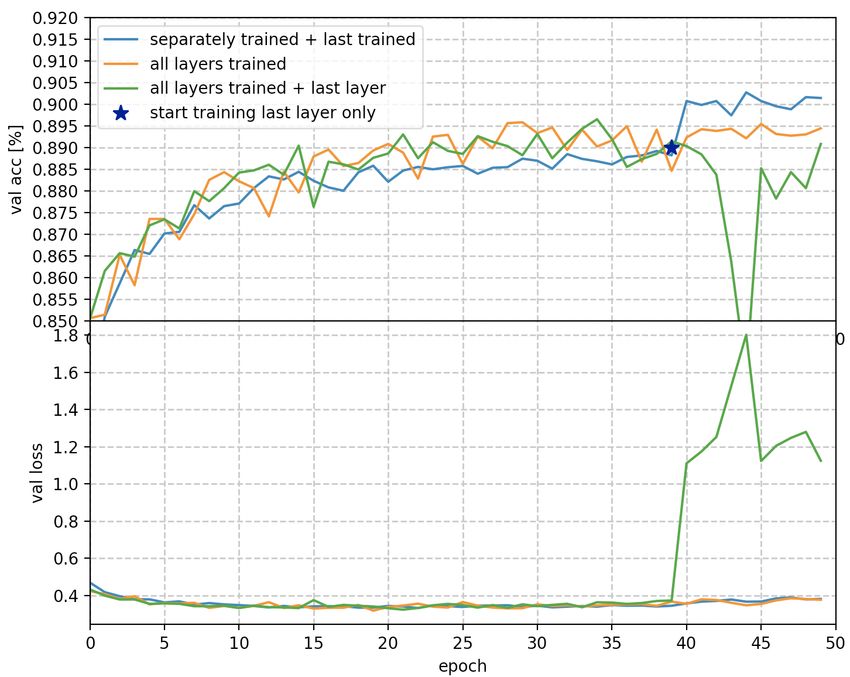
Acknowledgements
We would like to thank:

  1. A. Kolonko, P.Wandzel and K.Zuchniak, for their work resulting in promising
     preliminary results of SuperNet design which stimulate this thesis.

  2. ACK Cyfronet i PlGrid, for providing computing resources.

   The work was partially supported by National Science Centre Poland NCN:
project Number 2016/21/B/ST6/01539.

                                       ii
Contents
List of Tables                                                                                                                     iv

List of Figures                                                                                                                    iv

1 Introduction                                                                                                                      1
  1.1 Motivation and Thesis Statement                  .   .   .   .   .   .   .   .   .   .   .   .   .   .   .   .   .   .   .    1
  1.2 Structure of the thesis . . . . . .              .   .   .   .   .   .   .   .   .   .   .   .   .   .   .   .   .   .   .    1
  1.3 Contributions . . . . . . . . . . .              .   .   .   .   .   .   .   .   .   .   .   .   .   .   .   .   .   .   .    2
  1.4 Research Challenges . . . . . . .                .   .   .   .   .   .   .   .   .   .   .   .   .   .   .   .   .   .   .    2

2 Technological Background and Related Work                                                                                         3
  2.1 Machine Learning and Pattern Recognition . . . . . . . . . . . . . .                                                          3
  2.2 Ensemble and Stacked Generalization . . . . . . . . . . . . . . . .                                                           4
  2.3 Data and technical aspects . . . . . . . . . . . . . . . . . . . . . . .                                                      5

3 Network partitioning                                                                                                              7
  3.1 Last layers training . . . .     .   .   .   .   .   .   .   .   .   .   .   .   .   .   .   .   .   .   .   .   .   .   .    7
  3.2 Partitioning . . . . . . . .     .   .   .   .   .   .   .   .   .   .   .   .   .   .   .   .   .   .   .   .   .   .   .   11
  3.3 Loss function dilemma . .        .   .   .   .   .   .   .   .   .   .   .   .   .   .   .   .   .   .   .   .   .   .   .   16
  3.4 Best submodels . . . . . .       .   .   .   .   .   .   .   .   .   .   .   .   .   .   .   .   .   .   .   .   .   .   .   21
  3.5 Benefits of Supermodeling        .   .   .   .   .   .   .   .   .   .   .   .   .   .   .   .   .   .   .   .   .   .   .   24
  3.6 Summary . . . . . . . . .        .   .   .   .   .   .   .   .   .   .   .   .   .   .   .   .   .   .   .   .   .   .   .   26

4 Supermodeling of deep architectures                                                                                              28
  4.1 State of art results . . . . . . . . . . . . . . . . . . . . . . . . . . .                                                   28
  4.2 Loss surfaces analysis . . . . . . . . . . . . . . . . . . . . . . . . . .                                                   31
  4.3 Snapshot Supermodeling . . . . . . . . . . . . . . . . . . . . . . . .                                                       33

5 Conclusions and Future Work                                                                                                      36
  5.1 Summary and conclusions . . . . . . . . . . . . . . . . . . . . . . .                                                        36
  5.2 Future Work . . . . . . . . . . . . . . . . . . . . . . . . . . . . . . .                                                    36

Bibliography                                                                                                                       38

List of Tables
   1     Datasets . . . . . . . . . . . . . . . . . . . . . . . . . . . . . . . . .                                                 5
   2     Neural network architecture exploited in the thesis . . . . . . . . .                                                      6
   3     Training layers one-by-one . . . . . . . . . . . . . . . . . . . . . . .                                                   9

                                               iii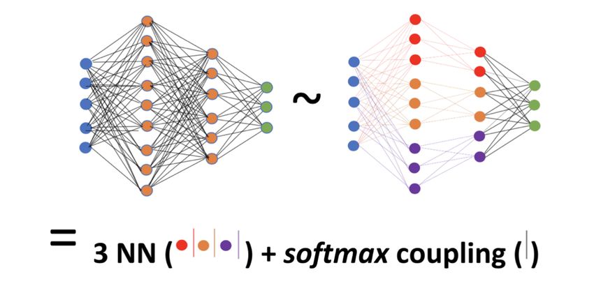
4    Network partitioning . . . . . . . . . . . . . . . . . . . .   .   .   .   .   .   .   14
  5    Supermodeling and loss measurements . . . . . . . . . .        .   .   .   .   .   .   18
  6    Last layer initializations of the NN ensemble . . . . . .      .   .   .   .   .   .   20
  7    Last layer trained for two models . . . . . . . . . . . . .    .   .   .   .   .   .   24
  8    Classical MLP vs SuperModel for Fashion MNIST . . . . .        .   .   .   .   .   .   26
  9    Classical MLP vs SuperModel for TNG . . . . . . . . . . .      .   .   .   .   .   .   26
  10   CPU time required for achieving 90% on Fashion MNIST           .   .   .   .   .   .   27
  11   CPU time required for achieving 84% on TNG . . . . . .         .   .   .   .   .   .   27
  12   Different number of submodels for an ensemble . . . . .        .   .   .   .   .   .   28
  13   FGE vs independent models . . . . . . . . . . . . . . . .      .   .   .   .   .   .   34
  14   FGE as quick accuracy boost . . . . . . . . . . . . . . . .    .   .   .   .   .   .   34

List of Figures
  1    DenseNet last layer training . . . . . . . . . . . . . . . .   .   .   .   .   .   .    8
  2    DenseNet predictions from penultimate layer . . . . . . .      .   .   .   .   .   .    9
  3    DenseNet predictions with last layer re-trained . . . . . .    .   .   .   .   .   .   10
  4    Last layers training for CIFAR10 dataset . . . . . . . . .     .   .   .   .   .   .   10
  5    Last layers training for CIFAR100 dataset . . . . . . . . .    .   .   .   .   .   .   11
  6    Network partitioning . . . . . . . . . . . . . . . . . . . .   .   .   .   .   .   .   12
  7    Different methods for last layer training for an ensemble      .   .   .   .   .   .   15
  8    Ensembling with sub-models coupling . . . . . . . . . .        .   .   .   .   .   .   16
  9    Loss-accuracy relation . . . . . . . . . . . . . . . . . . .   .   .   .   .   .   .   19
  10   Regularized ensemble . . . . . . . . . . . . . . . . . . .     .   .   .   .   .   .   20
  11   Supermodel at different epochs . . . . . . . . . . . . . .     .   .   .   .   .   .   21
  12   Loss for validation set for two models . . . . . . . . . . .   .   .   .   .   .   .   22
  14   Low and high loss vizualized . . . . . . . . . . . . . . .     .   .   .   .   .   .   23
  13   Loss for validation set for an ensemble . . . . . . . . . .    .   .   .   .   .   .   23
  15   Low and high loss visualized from penultimate layer . .        .   .   .   .   .   .   24
  16   SuperNet with different optimizers . . . . . . . . . . . .     .   .   .   .   .   .   29
  17   SuperNet on CIFAR10 . . . . . . . . . . . . . . . . . . . .    .   .   .   .   .   .   30
  18   SuperNet on CIFAR100 . . . . . . . . . . . . . . . . . . .     .   .   .   .   .   .   31
  19   Cyclic learning rate explained . . . . . . . . . . . . . . .   .   .   .   .   .   .   33
  20   Similarity matrix of independent models . . . . . . . . .      .   .   .   .   .   .   35
  21   Similarity matrix of FGE models . . . . . . . . . . . . . .    .   .   .   .   .   .   35

                                       iv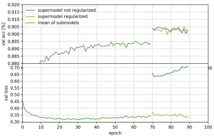
1     Introduction
1.1     Motivation and Thesis Statement
One can say that there is a trade-off between the computational budget used for
building neural networks and its final performance. Having in mind classification
problems, simple models achieve lower accuracy while the complex ones require
more CPU for training. Given the above, an interesting characteristic turn out
to have ensembles of pre-trained networks. They tend to achieve better results
than single models[1], and the gain increases, especially, when the base models
are significantly different. However, we still need additional resources to train the
base models(in this dissertation we will use the term: the sub-models). The in-
teresting question for that problem is whether we can have higher accuracy using
ensembles, compared to single networks, using the same amount of computational
budget. Inspired by the most recent researches around machine learning, we were
exploring the method of stacked ensembles of neural networks. We achieve the
ensemble by merging multiple sub-networks with the last layer, which we addi-
tionally train. We expect that such the architecture(we call it the Supermodel or
SuperNet) can improve prediction accuracy because the output of neural networks
is the most sensitive on the changes of weights from the last layer (see e.g., van-
ishing gradient problem). It can be time efficient as well, assuming that we can
train sub-models concurrently or obtain them as snapshots during the training of
a single network[2], [3]. The very preliminary results of such an approach were
initially presented at the V International AMMCS Interdisciplinary Conference,
2019[4]. Mainly, the primary motivation of my thesis was to:

    1. Prove that Supermodeling can be an efficient method for the accuracy im-
       provement of neural networks.

    2. Show the efficiency of Supermodeling method, concerning the CPU time.

    3. compare Supermodels to the classical networks of the same size.

    4. Investigate the method of obtaining sub-models for SuperNet as snapshots of
       training a single model.

1.2     Structure of the thesis
The first chapter gives a brief introduction to the theoretical background and the
latest achievements in the area of convolutional neural networks. We describe
the datasets used and the technical aspects of our research. In the second chap-
ter, we present a simple and efficient method for quick accuracy improvement of

                                         1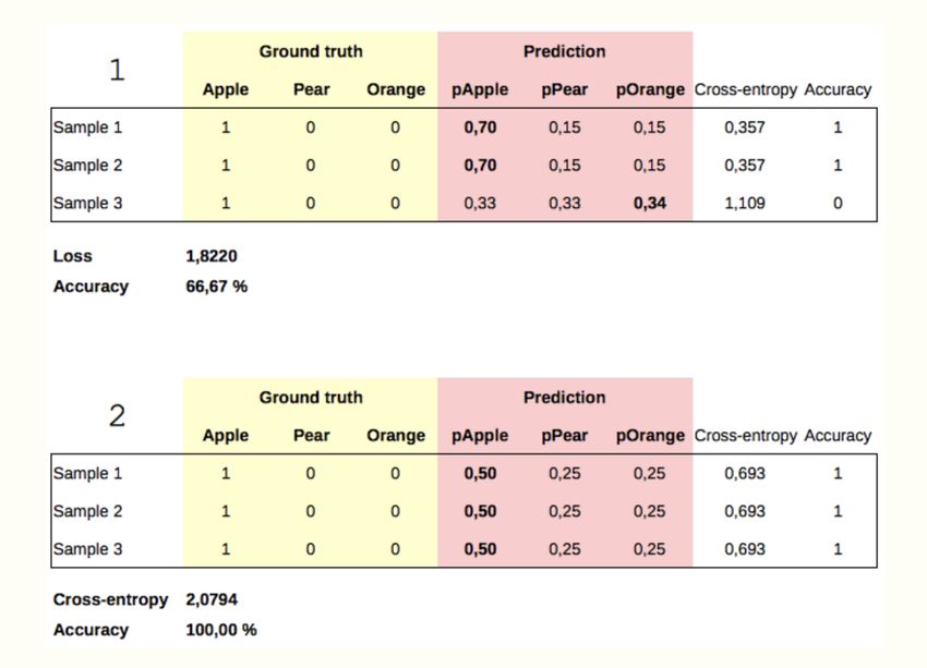
deep neural networks. We measure the properties of the ensembles built from
partitioned fully-connected networks. In the third chapter, we present the results
of Supermodeling for deeper architectures. In the fourth chapter, we show that
ensembles may be time-efficient when we consider novel methods for obtaining
submodels. The final chapter contains conclusions and the future work around
this subject.

1.3    Contributions
The contributions of the thesis are as follows:

  1. We present novel method for quick accuracy gain for the neural networks
     by training only its last layer only. We present the results for a few different
     architectures and datasets.

  2. We measure the performance of a partitioned network in comparison to a
     single model. We confirm the hypothesis that we can profitably replace very
     shallow dense networks with ensembles of the same size.

  3. We show that Supermodels of neural networks improve the accuracy. We
     achieve 92.48% validation accuracy on the CIFAR10 dataset and 73.8% on
     CIFAR100 which reproduce the best scores for the year 2015[5].

  4. We compare the accuracy of the Supermodel build from a) snapshots of train-
     ing a single network and b) the independently trained models. We present
     that such an approach can be efficient for deeper architectures.

1.4    Research Challenges
In my thesis, we are facing all the challenges related to the nature of classification
problems. Reliable studies in that branch require not only the basics of machine
learning but the knowledge of the newest achievements as well. The rapid increase
of the number of papers published in this domain shows its top importance for de-
velopment of artificial intelligence tools. Many of publications have very empirical
character. The lack of a formalized way of defining introduced solutions raises
many concerns. Considering the more technical aspect of our work, the training
of deep models is time-consuming, which takes even more resources when we
consider hyperparameters’s tuning and experiments on different datasets.

                                          2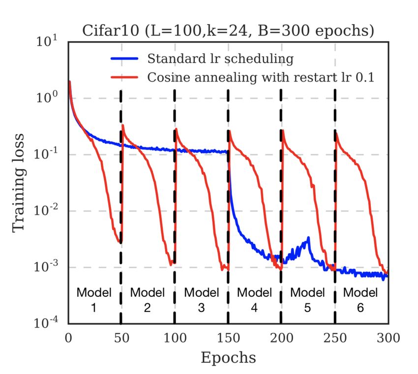
2     Technological Background and Related Work
2.1   Machine Learning and Pattern Recognition
In recent years, machine learning is the most rapidly growing domain of computer
science[6]. Neural networks prevail researchers’ attention due to new methods of
training and new type of architectures (deep, recurrent etc). Image recognition
is the field, in which lead convolutional neural networks. This trend started to
occur in 2012 with ImageNet-2012 competition’s winner, the AlexNet[7], which
showed the benefits of convolutional neural networks and backed them up with
record-breaking performance[8]. Inspired by that spectacular success, the next
years resulted in many architectures that focused on increasing accuracy even
more[9],[10], [11], [12]. The most straightforward solution for improvement
was to add more layers to the model[9], [10]. However, the multiple researches
had proven [12],[13],[14] that there are limitations of such method and very
deeper networks lead to higher error. One of the problems was that neural net-
work’s accuracy decreases over many layers due to vanishing gradient problem;
as layers went deep(i.e., from output to input due to backpropagation learning
scheme), gradients got small, leading to degradation. The interesting solution is
proposed in research "Deep Residual Learning for Image Recognition"[12]. The
Authors introduced residual connections which are essentially additional connec-
tions between non-consecutive layers. That simple concept significantly improves
the back-propagation process thus reduces training error and consequently allows
to train deep networks more efficiently. Moreover, a similar approach introduces
"Highway Networks"[15] paper, in which the Authors accomplished a similar goal
with the use of learned gating mechanism inspired by Long Short Term Mem-
ory(LSTM) recurrent neural networks[16].
    There is another important problem related to deep networks, called dimin-
ishing feature reuse problem, which was not solved in the described architectures.
Features computed by first layers are washed out by the time they reach the final
layers by the many weight multiplications in between. Additionally, more layers
results with longer training process. To tackle those complications, "Wide Residual
Networks"[17] were developed. The original idea behind that approach was to ex-
tend the number of parameters in a layer and keep the network’s depth relatively
shallow. Having that concept in mind, together with some additional optimiza-
tions (e.g., dropout[18]) the Authors achieved new state-of-the-art results on ac-
cessible benchmark datasets[5]. In the contrast to the idea of dedicated, residual
connections, the concept of "FractalNet"[19] was developed. The Authors tackle
the problem of vanishing gradients with an architecture that consists of multiple
sub-paths, with different lengths. During the fitting phase, those paths are being
randomly disabled, which adds the regularization aspect to the training. Their

                                        3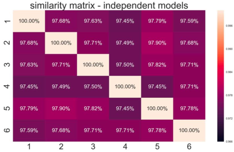
experiments reveal that very deep networks (with more than 40 layers) are much
less efficient than their fractal equivalents. The concept of disabling layers ex-
ploited "Stochastic depth"[20] algorithm. The method aims to shrink the depth of
the network during training while keeping it unchanged in the testing phase. That
was achieved simply by randomly skipping some layers entirely. Going through
the literature, one can observe that such concepts are often interpreted as specific
variations around network ensembles[21]. In the next paragraph, we would like
to focus on the concept of models ensemble.

2.2    Ensemble and Stacked Generalization
Ensemble learning is the machine learning paradigm of combing multiple learn-
ers together in order to achieve better prediction capabilities than constituent
models[1]. The technique address the "bias-variance" dilemma[22] in which such
an ensemble can absorb too high bias or variance of the predictions of its sub-
models and result in stronger predictor. The common types of ensembles are
Bagging[23], Boosting[24] and Stacking. The underlying mechanism behind Bag-
ging is the decision fusion of its submodels. The boosting approach takes advan-
tage of the sequential usage of the networks to improve accuracy continuously.
In our work, we are focusing on the last method - Stacking. Initially, the idea
was proposed in 1992 in the paper "Stacked Generalization"[25]. Conceptually,
The approach is to build new meta learner that learns how to best combine the
outputs from two or more models trained to solve the same prediction problem.
Firstly, we need to split the dataset into train and validation subsets. We indepen-
dently fit each contributing model with the first dataset, called level 0 data. Then,
we generate predictions by passing validation set through base models. Those out-
puts, named level 1 data, we finally use for training the meta learner. Authors of
[26] paper improved the idea with a k-fold cross-validation technique for obtain-
ing sub-models. In [27] it has been demonstrated that such a supermodel results
in better predictive performance than any single contributing submodel. Base sub-
models must produce uncorrelated predictions. The NN Stacking works best when
the models that are combined are all skillful, but skillful in different ways. We can
achieve it by using different algorithms.
    This brief introduction should help to understand what is the state-of-the-art
and the current challenges when building highly accurate and deep convolutional
neural networks(CNNs). In my thesis, we propose the ensemble architecture,
which we are going to describe and analyze in the following chapters.

                                         4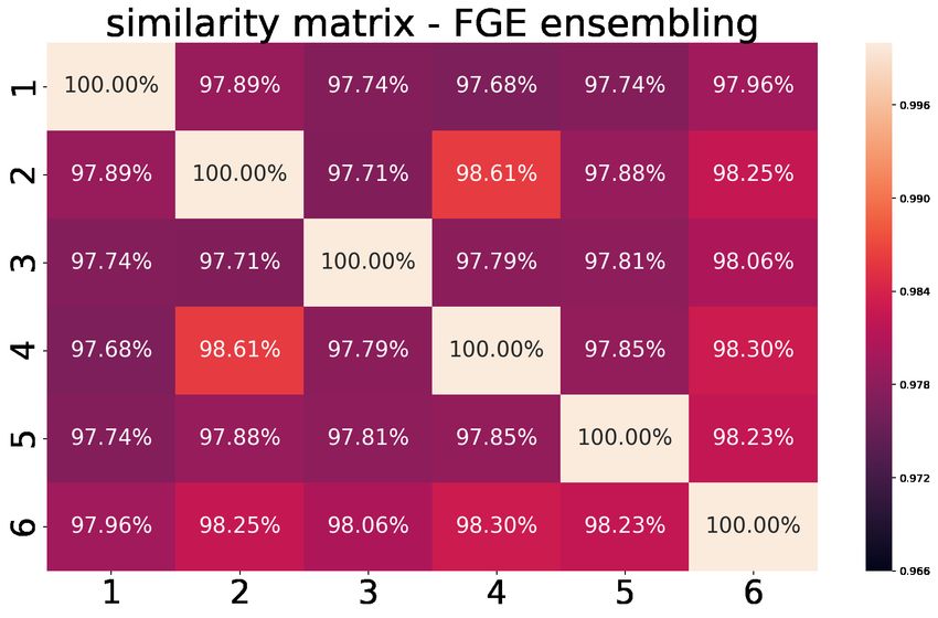
Table 1: Datasets used in my thesis.

                                 samples       input vector        classes
               CIFAR10           60,000        32x32x3             10
               CIFAR100          60,000        32x32x3             100
               Fashion MNIST     60,000        28x28               10
                                               text,
               Newsgroups20      20,000                            20
                                               different lengths

2.3   Data and technical aspects
For all of our experiments, we used the publicly available datasets that are com-
monly used as reference sets in the literature. It seems natural to use well-known
data so that the results could be easily replicated or compared with different anal-
yses. The datasets we are referring to are shwon in Table 1. The Table 2 presents
models used for experiments related to CIFAR10 dataset. Moreover, in the the-
sis we present the results on DenseNet[28], VGG-16[9] and multilayer percep-
trons(MLP). In our experiments, we are training a network on the training set and
validate the accuracy and loss on the validation set. For some experiments, we
isolated the testing set, which we used for final model evaluation. On most charts,
we present the validation accuracy and loss, as we regard them as more important
than the training curves. Training accuracy and loss always show an improve-
ment, which still may be overfitting though. All the code was written in Python3
and architectures modeled in Keras[29] library. The code was run on GPGPU on
the supercomputer Prometheus[30]. The CPU measured was the value returned of
the field CPUTime of sacct command run on Prometheus for the particular job.

                                           5
Table 2: Model used for experiments related to CIFAR10 dataset. Loss function was cate-
gorical crossentropy.
Layer Parameters Details
Input 32 x 32 x 3 CIFAR10 input image
Convolutional 32 (3x3) filters activation elu, batch norm, L2 reg α=0.0001
Convolutional 32 (3x3) filters activation elu, batch norm, L2 reg α=0.0001
MaxPooling 2x2 02. dropout
Convolutional 64 (3x3) filters activation elu, batch norm, L2 reg α=0.0001
Convolutional 64 (3x3) activation elu, batch norm, L2 reg α=0.0001
MaxPooling 2x2 0.3 dropout
Convolutional 128 (3x3) filters activation elu, batch norm,L2 reg α=0.0001
Convolutional 128 (3x3) activation elu, batch norm, L2 reg α=0.0001
MaxPooling 2x2 0.4 dropout
Fully Connected 10 activation softmax
63 Network partitioning
3.1 Last layers training
Reservoir computing[31] is a learning paradigm that introduces the concept of
dividing the system into input, reservoir, and readout components. The main
characteristic of such architecture is that only the readout weights are trained,
which significantly reduces the computational time. We ported that simple idea
into neural networks. We propose the training method, in which most of the time
we spend on fitting the whole model and then, we disable all the layers except
the last one. The remaining computational budget we use for training just the
last, active layer. The intuition behind that approach is the assumption that the
first levels of network are responsible for recognition rather simple features, like
angles or primitive shapes, hence are not learning significantly in the later stages
of the training. The preliminary results for such an approach started to look indeed
promising, as could be seen in Fig. 1. It illustrates validation accuracy and loss for
the training of DenseNet[28] architecture on CIFAR10 dataset and presents the
moments when we took snapshots of the network, and we trained only the last
layer.
Intrigued by that observation, we started applying additional fitting for the last
fully-connected layer, and up to the last two convolutional layers. Each time, we
fitted only one level of neurons, when we finished the training of the consequent
layers. The motivation behind the descending order was the assumption that the
gradients are better when the weights of successor neurons are more convergence
to the loss function’s optimum.
We have applied that method for six different pre-trained models from Table
2. We present the results in Table 3. The important note is that when we train
the layers in descending order, starting from the last one, we are achieving higher
accuracy. In that case, an additional 13 epochs improve the score of each network
by 2-5%. Having in mind that there is only one layer trained at the time, it tends
to overfit in a short amount of time. For that reason, only a few epochs should be
run at each stage.
To have a measure of the speedup of that approach, we have compared this
method to classical training in Figures 4 and 5 for datasets CIFAR10 and CIFAR100
respectively. As we can see, the additional accuracy gain is slowly decreasing over
the training time.
For a better understanding of the characteristics of the last layer’s training, we
were using visualization methods[32] of the network’s predictions. Firstly, in Fig.
2, we passed the whole testing set through a pre-trained DenseNet network, and
we captured the outputs from the penultimate layer. We observe that this fraction
of the model is enough to distinguish the classes correctly. In Fig. 3, we illustrate
7predictions of the whole network before, and after last layer re-train. After the
train, the clusters seem to be more concentrated, which confirms the improving
properties of this method. Those results also present the considerable difference
between the outputs of the last and penultimate layer, which may be a sign of the
significant role in the classification of the final level of neurons.
To conclude, "Freezing" all layers except the last ones speeds up the training
significantly. It can be used as a quick accuracy boost when we have limited re-
sources. It is a fascinating observation, and it is worth to do a separate study
around that method.
Figure 1: Validation accuracy and loss for 20 hours(around 80 epochs) of training
DenseNet model on CIFAR10 dataset. We applied additional training of only the last layer
for snapshots that we captured at 18, 30, 50, and 70 epoch of full network training. The
second gain(violet line) replicates the score that was achieved by full network training
more than 5h later. The accuracy achieved by the additional boost at 12th hour of train-
ing(red line) did not improve within the whole 20 hours of training. Nevertheless, most
likely, 20 hours was not enough time for the network to fully converge to its maximum
score. The axis is the CPU time spent on computations.
8Figure 2: We trained DenseNet model to achieve 93.62% on CIFAR10 dataset. Then, we
visualized[32] the outputs of the testing set from penultimate layer; each example was
980 dimensional vector. The numbers indicate CIFAR10’ classes.
Table 3: Validation accuracy for one-by-one layer training of six different models (2)
trained on CIFAR10. We can see that accuracy improves by 2-5% in just 13 additional
epochs.
last layer 2th layer from the end 3th layer from the end 4th layer from the end
base accuracy
(3 epochs) (3 epochs) (3 epochs) (4 epochs)
model 1 0.8548 0.8843 0.8929 0.8999 0.9035
model 2 0.8434 0.8791 0.8892 0.8944 0.8975
model 3 0.8619 0.8789 0.8854 0.8890 0.8949
model 4 0.8489 0.8812 0.8915 0.9007 0.9012
model 5 0.8636 0.8824 0.8913 0.8943 0.8978
model 6 0.8739 0.8871 0.8939 0.8927 0.8965
9(a) before last layer re-train. (b) after last-layer retrain.
Figure 3: This Figure presents the 2D embedding of the model’s (from Figure 2) predic-
tions for the test set before and after re-training of the last layer. The 5-nn metrics[32] are
0.906 and 0.912, respectively.
Figure 4: We have trained the model from Table 2 on CIFAR10 dataset and saved snap-
shots of 4,19,70 and 107 epochs. Then, we additionally trained the last four layers (one
layer at a time, starting from the last) of the snapshots. We trained each layer for four
epochs. The last blue dot indicates the maximum score of the base network without addi-
tional last layer training.
10Figure 5: We trained a VGG-16[9] model on CIFAR100 dataset for 250 epochs. We took
snapshots in the 15th,50th,100th and 200th epoch. Then, for those snapshots we trained
last four layers for 4 epochs each, one layer by one. The last fit improves accuracy for more
than 1%. Very close to SOTA obtained for VGG-16 (71.56%) in much shorter time[33].
3.2 Partitioning
Let us consider a dense network on which some internal connections between neu-
rons had been removed. Therefore, we can treat such a model as an ensemble of
multiple smaller networks. Fig. 6 should be helpful in understanding that obser-
vation. We have tested three different approaches for training the NN architecture
shown in Fig. 7, by training:
I. the whole network,
II. the whole network and additionally the last layer,
III. the subbranches independently and then merged them with the last layer,
which is additionally trained.
11Figure 6: If we remove some connections in a MLP network, it could be tread as an
ensemble.
Whereas the first two methods seem to yield similar or slightly better results than
training a single network, the SuperModel with re-trained last layer improves
the performance (Fig. 7). It may lead to a more generalized idea of creating
efficient networks. The construction of the architecture is as follows: multiple
dense networks that we trained on the same data are merged with the last, softmax
layer. For that purpose, we are copying the corresponding weights from the last
layers of subnetworks to the merged model and we are initializing biases to the
average values of corresponding biases. Fig. 8 shows how sample supermodel is
constructed. Then, inspired by the results from the previous chapter, we propose
to additionally re-train the last layer with the same training data for few(up to
10) epochs. From now on, each SuperModel in my thesis refers to the ensemble
with the re-trained softmax layer. In my thesis we use ReLu for internal activations
and softmax as output function for fully-connected networks. The reason behind
limiting the architecture type to multilayer perceptrons(MLP) in this chapter is that
it is possible to "cut alongside" such models and therefore combine the components
in SuperModel structures. The final model has the same amount of neurons in each
layer but less connections, which means less trainable parameters. That approach
gives many opportunities to compare the ensembles with the classical networks of
the same size.
As a next point of our research, we have divided Fashion MNIST dataset into
training, validation, and testing set and created three different sizes of dense
model. For each size, we have divided the MLP into 2, 3, 4, and 6 pre-trained
subnetworks and created SuperModel. We finished the training of each submodel
12by stopping it when the validation loss reached a specified threshed. The Ta-
ble 4 presents the accuracy and loss for the testing dataset with measured CPU
time. Those preliminary results demonstrate that the SuperModel indeed achieves
higher testing accuracy for bigger sizes of the architecture than corresponding
single models. Such an observation seems quite intuitive; ensembles result in bet-
ter performance but consume more CPU resources for training. In the rest of this
chapter, we would like to analyze the ensemble’s properties more deeply and focus
on how many benefits SuperModel can give.
13Table 4: Test accuracy and loss for networks that we partitioned into 2,3,4, and 6 subnet-
works. Each root model consisted of four layers:
Small network
subnetworks 1 2 3 4 6
test acc 0.8958 0.8906 0.8962 0.8943 0.8893
test loss 0.3194 0.344 0.3451 0.333 0.346
cpu time 00:01:49 00:02:04 00:03:19 00:03:48 00:06:01
Medium network
subnetworks 1 2 3 4 6
test acc 0.8942 0.8914 0.8971 0.8927 0.895
test loss 0.349 0.3445 0.3506 0.370 0.3659
cpu time 00:03:53 00:01:51 00:02:52 00:03:34 00:06:24
Large network
subnetworks 1 2 3 4 6
test acc 0.891 0.8983 0.8973 0.8953 0.8994
test loss 0.315 0.4026 0.404 0.405 0.424
cpu time 00:06:50 00:04:57 00:05:37 00:06:29 00:08:59
a) Small network: 360, 840, 840 and 10 neurons. We set dropout between layers
to 0.3 for single network and 0.2 for subnetworks. We finished the training of
single network when loss stopped to decrease for consecutive 10 epochs, and
for 5 epochs for subnetworks.
b) Medium network: 720, 1680, 1680 and 10 neurons. We set dropout between
layers to 0.3 for single network and 0.2 for subnetworks. We finished the
training of single network when loss stopped to decrease for consecutive 10
epochs, and for 5 epochs for subnetworks.
c) Large network: 1200, 2800, 2800 and 10 neurons. We set dropout between
layers to 0.7 for single network and 0.3 for subnetworks. We finished the
training of single network when loss stopped to decrease for consecutive 20
epochs, and for 10 epochs for subnetworks.
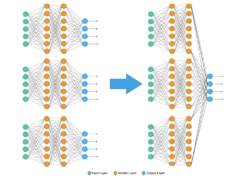
14Figure 7: Three different approaches for training architecture proposed in the Fig. 6
trained on Fashion MNIST dataset. The network consisted of four layers: (240, 560,
560,10) neurons, and we divided it into four subbranches. We used dropout with proba-
bility rate set to 0,1 between layers, ReLu as activation function and L2 regularization with
α=0.001.
I. orange line - we trained the whole network for 50 epochs.
II. green line - we trained the whole network for 39 epochs and then ten epochs
for only the last layer.
III. blue line - we trained four independent networks for 39 epochs, and then we
merged them with the last layer, which we additionally fit for ten epochs.
15Figure 8: Construction of SuperModel architecture from 3 sub networks. After the merge,
we additionally re-trained the last layer for short time with training data.
3.3 Loss function dilemma
During our experiments around the Supermodeling on different datasets, we have
always observed one striking issue. Although the validation accuracy of such an
ensemble is higher than the corresponding submodels, the testing/validation loss
tends to be higher as well (Table 4). The overfitting is the most common answer to
that behavior. We have a slightly different interpretation for that phenomenon. In
our opinion, it results from the loosely coupled nature between softmax loss func-
tion and its finally predicted class. Figure 9 may help to understand this relation.
There may be two scenarios happening at the same time. Firstly, the ensemble is
overconfident of its predictions which results in increased error loss for incorrect
guesses. At the same time, the border examples (the examples that networks is not
16sure about) are predicted better, which improves the score. If the first case hap-
pens often enough, the loss function will grow with untouched accuracy, which is
additionally "bumped" by the second scenario. In order to prove this hypothesis,
we measured the basic properties of SuperModel and its corresponding subnet-
works in Table 5. Indeed the SuperModel has a higher mean loss, but 90% of the
examples reach a minimal error. When we interpret this together with the bigger
standard deviation, we can conclude that the mean error is increased mostly by
the remaining 10% of guesses. Overconfidence means that the output probabilities
are closer to the edge values (0 and 1); therefore, the incorrect predictions lead to
very high cross-entropy. Moreover, the 95th percentile shows much higher value
which we can explain by the fact that it is more than the accuracy of the Super-
Net(91%) thus the remaining 4% must be wrong guesses that generate very high
error (Table 5). It is known that overconfident predictions may be the symptom
of overfitting[34]. However, we need to keep in mind that creating an ensemble
we are actually building a new model with different capabilities, whereas overfit-
ting is related to the process of training a single model. In our experiments, the
regularization method of L2 penalty added to weights in the stage of training the
last layer reduces the loss significantly. On the other hand, it usually had smaller
final accuracy of the ensemble in comparison to non-regularized ensembles. To
have a better insight, Table 6 presents validation accuracy and loss for training
SuperModel’s softmax’s layer on two different datasets. In Table 6, we compared
three different initializations of last layer’s weights - a) when the coefficients are
initialized in random, b) when we directly copied the corresponding weights from
the submodels and c) when we copied the weights and additionally re-scaled them
by dividing by an arbitrary factor. The intuition behind the last case comes from
the conclusion that the overconfidence, which we observed, is occurring when the
weights reach high values. Building SuperModel, we are combining connections
for the last layer from multiple submodels. If the activations for the same feature
are similar in each model (e.g., each corresponding neurons give similarly nega-
tive value for a particular example) then the final value is proportionally higher. To
prevent this effect, we have reduced the coefficients with division operation. We
have repeated the experiment on models of different sizes and we very often came
up with the same conclusion that is the highest score (accuracy and loss) achieves
the non-regularized training of the last layer on which the coefficients were copied
and down-scaled. However, we did not come up with a standardized way of nor-
malizing the weights, and we were choosing the factors experimentally. The less
intuitive is the fact that the best division factor was sometimes much bigger than
the number of subnetworks(e.g., 60), depending on the model. Nevertheless, as
shwon in Fig. 10, the difference is not that huge, and in some cases, choosing reg-
ularization parameters carefully still decreased the error, without impacting the
17precision of the outputs.
In our opinion, using Supermodeling with randomly initialized weights and
regularization may be a feasible way of increasing the network’s performance
enough, so that we can keep proper accuracy/loss balance. We think that cop-
ing the weights from submodels should not be a necessary step and we suspect a
trivial reason why it worked in our experiments. Each time, we were initializing
a new optimizer for the last layer training, which forced the coefficients to move
dramatically, hence their initial state was not that important. The problem of the
Supermodel’s high confidence and its response to regularization is tightly related
to the level of variance of the submodels that we combine. This is the topic that
we try to address in the next paragraph.
Table 5: Evaluation of six models and their SuperModel on the validation set. Each sub-
model was a fully-connected network that we trained on FMNIST dataset and had the
architecture of four layers(200, 466, 466 and 10 neurons). SuperModel achieves better
accuracy despite the higher mean loss. However, the 90% of the predictions have small
errors. Based on this fact, one can conclude that the high mean value results from very
few predictions that were overconfident and incorrect.
accuracy loss mean loss std loss 90th loss 95th
6 Submodels (average) 0.89315 0.65722 2.4633 0.92668 4.4884
SuperNet 0.9103 1.0976 3.8482 0.06541 16.11809
18Figure 9: Example that presents the scenario that the lower loss of softmax function does
not always mean the lower score in general. Even though the second predictor outputs
lower probabilities (it’s "less sure"), his final accuracy is higher[35].
19Figure 10: SuperModel created from models trained on Fashion MNIST Dataset. The
submodels were fully-connected networks with four layers: (120, 280, 280, 10) neurons.
For both trainings, we copied the corresponding weights directly from submodels into
Supermodel. L2 regularization added to weights and bias during SuperModel’s training
reduces the error without accuracy drop(orange line).
Table 6: We have compared a few different approaches for SuperModel’s last layer initial-
ization on two datasets. The presented values are Validation accuracy/Validation error for
the best score achieved(for about 20 epochs of the softmax layer training). For Fashion
MNIST six subnetworks were pretrained, each 200, 466, 466 and 10 neurons. For TNG
dataset six subnetworks were pre-trained, each 30, 30 and 10 neurons. For the downscale,
we chose the factors experimentally. The worst loss achieves the non-regularized weights
directly copied from the submodels.
Fashion MNIST TNG
random copied weights random copied weights
init downscaled not scaled init downscaled not scaled
0.9122/ 0.9132/ 0.9112/ 0.8385/ 0.8502/ 0.8458/
non-regularized
0.6401 0.7633 1.1066 0.9216 0.6651 1.3965
L2 penalty, 0.9105/ 0.9088/ 0.9089/ 0.8424/ 0.8484/ 0.8410/
alfa=0.01 0.4187 0.4295 0.5079 0.6988 0.6433 0.7225
L2 penalty, 0.9113/ 0.9102/ 0.9105/ 0.8429/ 0.8497/ 0.8467/
alfa=0.001 0.5207 0.5599 0.5705 0.8208 0.6678 1.4009
203.4 Best submodels
A good entry point to this paragraph will be Fig. 11.
Figure 11: The SuperModel created at 20, 40 and 60th epoch of training 6 models on
Fashion MNIST dataset. Each model had architecture of four layers; 40 60, 60 and 10
neurons. Even though it seems that the base models are getting overfit (regularization
was not used), the Supermodel created at the latest stage of the training appears to have
the highest score.
For that experiment, we have pre-trained six sub-models on Fashion MNIST
data. We were building a SuperModel at 20, 40 and 60th epoch of the models’
training. Unusual is the fact that the accuracy achieved by the ensemble from
the 60th epoch has the higher score than one from the 20th epoch, even though
the submodels have very similar accuracy in both points. Moreover, it seems that
the base models are getting overfitted, as the accuracy is stable, but loss slowly
increases. Our explanation for this phenomenon is that the ensemble has more
accurate guesses when the submodels are more overconfident. We have plotted
loss outputs for each validation example, respectively for one model from 20 epoch
and from the 60th one.
In Fig. 12 it is visible that the 20th epoch’s model has more balanced predic-
21(a) 20 epoch (b) 60 epoch
Figure 12: The loss outputs for each example from validation set of Fashion MNIST for
two sample snapshot models taken respectively from 20 and 60 epoch of the training a
single model(one of the models from Fig. 11). Please note that the scale is logarithmic.
tions with less variance. The latter, more overconfident model has outputs that are
more close to discrete guesses. Thus, the 60th epoch’s predictions are either very
precise or completely wrong. In Figures 14 and 15 we visualized[32], [36] the
outputs for the whole test set for the same two models, from last and penultimate
layer respectively. Whereas the 5-nn metric for last layer embedding was bigger
for the model with lower loss(0.846 and 0.829), the outputs from penultimate
layers had a similar metric, equal 0.866. This result suggests that the high error
of the 60th epoch’s model is generated mostly by its final layer. It explains why
SuperModel for 60th epoch models is not worse than 20th epoch models; when
we build an ensemble, we forget the old coefficients of the last layers for each
submodel and learn new ones. Analyzing the 5-nn metric from Fig. 15 further,
we conclude that model from 60th epoch with re-trained last layer should end up
with slightly better accuracy. We confirm such results in Table 7. The loss lines
from 11 suggests that the overconfidence of submodels implies higher overconfi-
dence of the ensemble as well. To demonstrate that, Fig. 13 presents loss for each
validation example of the Supermodel created from 60th epoch of the submodels’
training. The bars are either very short or long, which means almost "black or
white" guesses. We can conclude that when choosing the submodels for an ensem-
ble, there is a trade-off between the reliability and accuracy of the Supermodel’s
predictions.
22(a) 20 epoch. Acc: 0.8954.
(b) 60 epoch. Acc: 0.886.
5-nn acc: 0.846
5-nn acc: 0.829
Figure 14: Visualization of the predictions for each example from the validation set of
Fashion MNIST for two sample snapshot models taken respectively from 20 and 60 epoch
of the training a single model(Fig. 11). The 5-nn metric was equal 0.846 for 20th epoch
and 0.829 for 60th epoch.
Figure 13: The loss outputs for each example from validation Fashion MNIST dataset for
the Supermodel created from submodels from the 60th epoch of training a single model
(one of the models from Fig. 11). The scale is logarithmic.
23(a) 20 epoch. 5-nn acc: 0.866 (b) 60 epoch. 5-nn acc: 0.867
Figure 15: Visualization of the outputs from the penultimate layer for each example from
the validation set of Fashion MNIST for two sample snapshot models taken respectively
from 20 and 60 epoch of the training a single model(Fig. 11). Surprisingly, the 5-nn
metric was similar in both cases, equal 0.866 for 20th epoch and 0.867 for 60th epoch.
Table 7: We trained only last layer for two models; from 20th and 60th epoch of the
training. We randomly initialized the weights for last layer and used L2 regularization
with alfa equal 0.01 during the training.
before training last layer after training last layer
val_acc val_loss val_acc val_loss
epoch 20 model 0.8954 0.396 0.8961 0.3765
epoch 60 model 0.886 0.682 0.8994 0.4175
3.5 Benefits of Supermodeling
Let us assume that we have trained the model already, but we would like to re-
duce the number of parameters without decreasing its final score. The motivation
behind this approach might be that the final model is supposed to be uploaded on
an embedded device(limited disk space), or we wish to speed up the prediction
process. The assumption is that we are still in the process of fine-tuning the archi-
tecture. There are existing methods [37] proposed for a neural network compres-
sion; however, all of them consider that we are operating on the weights of already
pre-trained models. In this paragraph, we try to answer the question, whether Su-
permodeling could be used to compress the architecture before the training.
In Table 8, we have compared the performance of SuperModel with the normal
network that has the same size in terms of weights’ space. The results demon-
24strate that the ensemble achieves better results, starting from a certain size of
the model. We can conclude that after reaching some threshold, we can have a
higher gain with Supermodeling approach for shallow networks. However, it may
be still possible that properly tuned hyperparameters of a single network may pro-
duce better results. Especially for bigger models, in order to prevent overfitting
the regularization methods like L2 norm or dropout[18] should be used. After
playing a bit with hyperparameters and extending the training time significantly,
the best score that we were able to achieve for Fashion MNIST dataset for a sin-
gle network was 90.8%(480, 1120, 1120 and 10 neurons), whereas SuperModel
reached 91.36 % (6 subnetworks, 200, 466, 466 and 10 neurons each). We have
performed similar experiments on TNG dataset in Table 9. We have trained the
classical models for up to 200 epochs and captured the best score. Having in
mind that dropout achieves similar performance as L2 norm[38], we compared
ensembling only with dropout For each size, we chose the most optimal model’s
configuration, based on the manipulation of the dropout rate in each layer. The
depth of networks was always 3 levels of neurons. Based on high loss, it looks
like the single network was reaching its best score being overfitted. In this exper-
iment, the SuperModel’s weights were rescaled before training, because it reduces
the loss due to results from Loss function dilema paragraph. Especially, for the
models of bigger sizes, we have received the highest score of around 84% when
the dropout rate was large, around 0.7. We would like to recall that one of the
explanations why using the dropout technique works, is that it may be perceived
as an aggregation of the exponential number of ensembles[18],[39] in a single
model, however, trained independently only one epoch. Thus, the dropout gains
from averaging properties of the ensembles, which reduce the variance and pre-
vents from overfitting. Significant difference between these two concepts is the
measure of correlation between neurons. The neurons from two submodels in the
ensemble are disconnected, whereas dropout "generates" tightly coupled submod-
els, with shared weights. This is just a specific point of view on dropout, and for
further reading, please refer to the literature[40]. Analyzing the results from Ta-
bles 8 and 9, it appears that the ensemble learning achieves better results, notably
for bigger models. We hypothesize that starting from a certain level of model’s
complexity, the Supermodeling gives a better correlation degree between the fea-
ture detector units(understood as neurons or group of neurons) than hypothetical
ensembles "created" by standard dropout approach[41]. In less correlated ensem-
bles, the units are more independent and do not share that much information. This
may lead to the conclusion that the Supermodeling could be used to regularize very
shallow and wide networks by sort of structure modification during training. This
would partially explain why convolutional networks work so well as the gain come
from separate autonomous filters. However, in order to prove such the hypothe-
25sis, a separate study would be necessary, and our conclusions are rather intuitive
guesses than formally proved theorems. We did not use the word "compression"
here on purpose - it would imply that the classical network always reproduces the
score of the Supermodel. However, that was not a case, and we did not manage
to achieve the same result of 85% on TNG dataset and 91% on F-MNIST with the
classical model of any size. Obviously, that may be the matter of perfectly chosen
hyperparameters and regularization. Therefore, the Supermodeling seems to be a
more natural and quicker way for trivially boosting performance without spending
much effort on the architecture’s fine-tuning.
Table 8: Validation accuracy for 7 different sizes of classical networks and corresponding
SuperModels for 100 epochs of training on Fashion MNIST dataset. The base model had
53k trainable parameters and consisted of four layers; 45, 105, 105, and 10 neurons. We
set dropout rate to 0.2 between layers. We scaled the model by multiplying the number
of neurons in each layer by different factors, which produced seven different architec-
tures(each column). Then, each model was compared with two types of SuperModels (6
submodels) that had a similar number of parameters and the same 4-layers depth. The
score of the Supermodel trained from completely random initialization proves that it is not
that good as when we trained subnetworks separately (already shown in the Fig. 7);
number of parameters 53 k 115 k 360 k 687 k 1,257 k 1,781 k 2,837 k
Classical MLP 0.8826 0.8928 0.9023 0.9057 0.9049 0.9074 0.9054
SuperModel 0.8559 0.8724 0.8941 0.9025 0.9071 0.9081 0.9113
SuperModel whole trained 0.8845 0.8947 0.9018 0.9038 0.9025 0.9016 0.9039
Table 9: Validation accuracy for 7 different sizes of classical networks and corresponding
SuperModels training on TNG dataset.
number of parameters 300k 600k 1,15 kk 1,81 kk 3,09 kk 5,15 kk 7,3 kk
val_acc 0.8129 0.8185 0.8343 0.8445 0.8406 0.8437 0.8426
Single model
val_loss 0.7637 0.7144 0.7051 1.0552 0.9098 1.6795 1.5173
val_acc 0.8016 0.8261 0.8348 0.8502 0.8465 0.8504 0.8470
SuperModel
val_loss 0.7585 0.7686 0.6600 0.6649 0.9174 0.8600 0.7480
3.6 Summary
Summarising what we presented in this chapter:
1. In the "Last layers training" section, we have introduced a novel method for
boosting the accuracy of a single NN model.
2. Then, the "Partitioning" section proposes the specific ensembling method that
improves the classification performance by combining multiple submodels of
the partitioned network
263. In the section "Loss function dilemma", we explain why increasing valida-
tion accuracy does not always come together with decreasing loss for cross-
entropy function.
4. In the section "Best submodels", we presented that slightly overconfident net-
works create compositions that are more accurate and confident.
5. "Benefits of Supermodeling" points out that the efficiency of the ensemble
method differs from the classical models depending on the scale of parame-
ters.
Let us recall the Table4 from the introduction of this chapter. We concluded
that the ensemble achieves a higher score than a single network, but it is more
time-consuming. However, to prevent overfitting, the training of the subnetworks
was terminated when the validation loss stopped to decrease. At this last stage of
our research around partitioning fully-connected networks we would like to com-
pare the CPU time of the Supermodel and an individual model until both reached
the same validation accuracy, regardless of the architecture and size. We fine-
tuned single model and an ensemble in order to achieve 90% precision on Fashion
MNIST and 84% on TNG. We present the results in Tables 10 and 11. We conclude
that ensembling can be used for saving CPU resources as well. However, we need
to keep in mind that all those experiments were done on MLP networks, and con-
volutional architectures could achieve greater scores on the mentioned datasets —
results from convolutional types of networks we present in the next chapter.
Table 10: We compare CPU time required for reaching 90% accuracy on Fashion MNIST
for a best individual model and an ensemble. The Supermodel consisted of 3 subnetworks
and was significantly faster.
val acc val loss time
single net 0.9 0.3228 00:08:36
supermodel 0.9 0.3198 00:04:59
Table 11: We compare CPU time required for reaching 84% accuracy on TNG for a best
individual model and an ensemble.
val acc val loss time
single net 0.84 1.1336 00:03:00
supermodel 0.84 0.6508 00:01:13
27Table 12: Accuracy of the SuperNet and Softmax voting with respectively 6,5,4,3,2 and 1
subnetworks included for CIFAR20 dataset and the model from Table 2. The results show
that more pre-trained submodels effect in better SuperNet’s accuracy.
Models 6 submodels 5 submodels 4 submodels 3 submodels 2 submodels 1 submodel
model1 acc 0.8636 0.8636 0.8636 0.8636 0.8636 0.8636
model2 acc 0.8619 0.8619 0.8619 0.8619 0.8619 -
model3 acc 0.8548 0.8548 0.8548 0.8548 - -
model4 acc 0.8489 0.8489 0.8489 - - -
model5 acc 0.8434 0.8434 - - - -
model6 acc 0.8739 - - - - -
SuperNet 0.9120 0.9104 0.9083 0.9044 0.901 0.8894
Softmax 0.8973 0.8904 0.8925 0.8892 0.8832 0.8636
4 Supermodeling of deep architectures
4.1 State of art results
Setting aside the considerations around MLP models, we have experimented with
Supermodeling of deep architectures. For that part of experiments, we used CI-
FAR10 and CIFAR100 datasets[42] and model presented in Table 2. Fig. 16
demonstrates the results of validation accuracy and loss for four independently
trained NN models(we call it here, in contrast to the previous "partition" Super-
Models, SuperNets). Each network was trained up to 200 epochs with varoius
optimizers: adagrad, rmsprop, nadam, and adam. This is important because as
shown in [43], the quality of trained NN model depends heavily on the optimiza-
tion method used. The best choice, in turn, depends on both dataset considered
and the NN architecture employed. After the training, we have created the Su-
perNet and additionally fit the last layer. Figures 17 and 18 present the results
of SuperNet of six models in different stages of the training for CIFAR10 and CI-
FAR100 datasets respectively. The results present that SuperNet wins over the
classical voting ensembles. In Table 12 we have measured the SuperNet’s scores
for different numbers of subnetworks. Based on Table, we can conclude that the
higher number of models implies the better accuracy of their SuperNet. We ad-
ditionally implemented the idea of re-training just the last layers for those six
submodels and after that combined them into the SuperNet. We achieved 92.48%
validation accuracy on the CIFAR10 dataset. This result reproduces the best score
for the year 2015 for that particular dataset[5], which is quite impressive as we
are considering an ensemble of rather simple convolutional networks.
28Figure 16: Validation accuracy and loss of training four models from Table 2. Blue dot in-
dicates the accuracy achieved by SuperNet created from those models. We do not present
SuperNet’s training time because it is significantly shorter than subnetworks, as we train
only the last, fully-connected layer. Usually, it takes less than ten epochs, and it is overfit-
ting sensitive.
29Figure 17: SuperNet based on six models, saved in 10,40, 70 and 110 epoch of training on
CIFAR10 dataset for a model from Table 2. The same optimizer Adam was used for each
network. The result is compared to Majority voting method and Softmax voting. Softmax
voting is the voting based on the sum of probabilities outputs from the subnetworks. The
results are from different training than values presented in Table 12.
30Figure 18: SuperNet based on six models, saved in 50,100, and 150 epoch of training on
CIFAR100 dataset for VGG[9] model. The result is compared to Majority voting method
and Softmax voting.
4.2 Loss surfaces analysis
We have already proven in Table 12 that we a better improvement for an ensemble
occurs when we include a higher number of submodels. However, we know that
having multiple pre-trained networks is computationally expensive, as we need
to train them independently. Finding diverse networks easily is not a trivial task
but already addressed in the literature[2], [3]. If we think about neural network
training from a geometrical point of view, the goal is to find a global minimum
in the highly dimensional surface of a loss function. The shape of the surface de-
pends on multiple factors like the chosen model, number of trainable parameters,
dataset, and more. There are multiple studies around the topic of visualization
landscapes[44] of the loss functions and the analyses of them [45],[46].
In my thesis, we would like to put more attention on one - "Loss Surfaces, Con-
nectivity Mode and Fast Ensembling of DNNs"[3] by Timur Garipov. The author
discovers the fascinating property of the surfaces of the deep neural networks.
His empirical researches present that every two local optima are connected by
the simple curves or even triangle polyline over which training and test accu-
31racy are nearly constant. The interesting is the fact that the independent re-
search team[47] discovered the same property of the multidimensional loss func-
tion’s surface. Their approach was based on the Automated Nudged Elastic Band
algorithm[48], which addresses problems related to physics and chemistry. That
leads to the conclusion that is just one pre-trained network could lead, without
large computational budget, to an infinite number of other, diverse networks with
similar performance. It comes from the assumption that our network is located
in some "valley" of low loss error. Moreover, Garipov in [3] proposes a unique
method of training neural networks, called Fast Geometrical Ensemble(FGE), that
finds such models and ensemble those snapshots in order to achieve improved ac-
curacy. Inspired by the geometrical insights, the approach is to adopt a cyclical
learning rate that forces the optimizer (e.g., gradient descent) to "travel" along
mode connectivity paths. Even though it is not the first introduction of cyclical
learning rate in the domain literature([49], [2]), the author highlights that his
method uses a very small cycle compared to other works and finds diverse models
relatively faster.
The general idea behind such a cyclic learning rate, sometimes called cosine
annealing learning rate, is to assume that we have a cycle that consists of a constant
number of epochs. Each cycle starts with a relatively large learning rate, which is
consequently decreased with the training time. At the end of the cycle, it should
be comparable to a standard learning rate. Then, one saves the snapshot of the
model and starts the process again. We present in Fig. 19 a comparison of training
loss of standard learning rate and cyclic learning rate on DenseNet. In the next
paragraph, we are testing such a method for obtaining submodels for our ensemble
architecture.
32Figure 19: Training loss of standard learning rate and cyclic learning rate on
DenseNet[28], on CIFAR10. We took a figure from "Snapshot ensembles: Train 1, Get
M for Free"[2]
4.3 Snapshot Supermodeling
We compare an accuracy reached by an ensemble that we built from submodels
achieved by FGE[3] method in Table 13. We conclude that FGE method does not
bring diverse models as independent training. However, still, the gain of Super-
modeling of such the models is notable. There are various studies [50] around the
topic of diversity of models combined into ensembles. In my thesis, we recall the
results of Konrad Zuchniak[51], which present similarity matrices, measured as
percentage of the examples classified to the same class by two models. Figures 20
and 21 illustrate matrices for independently trained models and FGE snapshots,
respectively. We observe that the FGE snapshots are less diverse, which explain
why their Supermodeling does not perform that well as in comparison to indepen-
dently trained models. As of the last experiment, we combined all the optimization
methods mentioned in my thesis, to achieve a score of 90% on CIRAR10 dataset
33You can also read