Supersonic mode in a low-enthalpy hypersonic flow over a cone and wave packet interference
←
→
Page content transcription
If your browser does not render page correctly, please read the page content below
Supersonic mode in a low-enthalpy
hypersonic flow over a cone and wave
packet interference
Cite as: Phys. Fluids 33, 054104 (2021); https://doi.org/10.1063/5.0048089
Submitted: 19 February 2021 . Accepted: 21 April 2021 . Published Online: 13 May 2021

  Christopher Haley, and Xiaolin Zhong

ARTICLES YOU MAY BE INTERESTED IN

Mechanism of stabilization of porous coatings on unstable supersonic mode in hypersonic
boundary layers
Physics of Fluids 33, 054105 (2021); https://doi.org/10.1063/5.0048313

Ab initio simulation of hypersonic flows past a cylinder based on accurate potential energy
surfaces
Physics of Fluids 33, 051704 (2021); https://doi.org/10.1063/5.0047945

Influence of corner angle in streamwise supersonic corner flow
Physics of Fluids 33, 056108 (2021); https://doi.org/10.1063/5.0046716

Phys. Fluids 33, 054104 (2021); https://doi.org/10.1063/5.0048089                       33, 054104

© 2021 Author(s).
Physics of Fluids                                                                                ARTICLE           scitation.org/journal/phf

    Supersonic mode in a low-enthalpy hypersonic
    flow over a cone and wave packet interference
    Cite as: Phys. Fluids 33, 054104 (2021); doi: 10.1063/5.0048089
    Submitted: 19 February 2021 . Accepted: 21 April 2021 .
    Published Online: 13 May 2021

    Christopher Haleya)               and Xiaolin Zhongb)

    AFFILIATIONS
    Mechanical and Aerospace Engineering Department, University of California, Los Angeles, California 90095, USA

    a)
         Author to whom correspondence should be addressed: clhaley@g.ucla.edu
    b)
         Electronic mail: xiaolin@seas.ucla.edu. URL: http://cfdhost.seas.ucla.edu/

    ABSTRACT
    A computational fluid dynamics study is conducted in which acoustic-like waves are observed emanating from the boundary layer of a Mach
    8 slender blunt cone with a relatively low freestream enthalpy and a warm wall. The acoustic-like wave emissions are qualitatively similar to
    those attributed to the supersonic mode. However, the supersonic mode responsible for such emissions is often found in high-enthalpy flows
    with highly cooled walls, making its appearance here unexpected. Linear stability analysis on the steady-state solution reveals an unstable
    mode S (Mack’s second mode) with a subsonic phase velocity and a stable mode F whose mode F- branch takes on a supersonic phase veloc-
    ity. It is thought that the stable supersonic mode F- is responsible for the acoustic-like wave emissions. Unsteady simulations are carried out
    using blowing-suction actuators at two different surface locations. The analysis of the temporal data and spectral data using Fourier decom-
    position reveals constructive/destructive interference occurring between a primary wave packet and a satellite wave packet in the vicinity of
    the acoustic-like wave emissions. The constructive/destructive interference between the wave packets also appears to have a damping effect
    on individual frequency growth in both unsteady simulations. Based on this study’s results and analysis, it is concluded that a supersonic dis-
    crete mode is not limited to high-enthalpy, cold wall flows and that it does appear in low-enthalpy, warm-wall flows; however, the mode is
    stable.
    Published under an exclusive license by AIP Publishing. https://doi.org/10.1063/5.0048089

    I. INTRODUCTION                                                             condition and an associated wave packet interference pattern between
          Hypersonic boundary layer transition research is an essential         primary and satellite waves. While performing a computational study
    area of investigation because turbulent boundary layers can increase        on surface roughness’s ability to attenuate Mack’s second-mode insta-
    surface heating by a factor of 4–10, which necessitates the application     bility,7 the acoustic-like waves seen in Fig. 1 were observed emitting
    of heavy thermal protection strategies.1,2 Transition, however, is a pro-   from the boundary layer in an unsteady simulation with no surface
    cess with multiple pathways leading to turbulence, as described by          roughness. These acoustic-like waves are qualitatively similar to those
    Morkovin et al.3 This paper is concerned with the pathway associated        seen by Chuvakhov and Fedorov,8 and Knisely and Zhong5,6,9,10 in
    with low environmental forcing, which is typified by discrete normal         their direct numerical simulation (DNS) investigation of supersonic
    modes such as the fast and slow modes (modes F and S). These dis-           modes. Despite the similarities between the observed phenomena, the
    crete modes are responsible for the well-known Tollmien–Schlichting         simulation conditions are very different; the supersonic mode reliably
    waves and Mack’s second-mode instability, and most recently, by a           appears in flows with cooled walls, which makes the appearance of
    renewed interest in supersonic modes. Recent research into supersonic       similar acoustic-like waves in a flow with a warm-wall unexpected.
    modes has shown that unstable supersonic modes can contribute to                  Supersonic modes were first described from Mack’s numerical
    Mack’s second mode and increase the boundary layer’s overall insta-         investigations in 1984,11 1987,12 and 1990,13 and by Reshotko in 1991.14
    bility.4–6 For this reason, it is important to know under what physical     Mack showed there exist discrete neutral waves whose phase velocity
    conditions supersonic modes appear and their underlying physical            caused the wave to propagate supersonically relative to the flow at the
    mechanism, which is not currently well understood.                          boundary layer edge, such as when the discrete wave’s phase velocity, c,
          This paper investigates acoustic-like emissions from the bound-       is less than the propagation speed of a slow acoustic wave, u  a. In
    ary layer of a low-enthalpy flow over a Mach 8 cone with a warm-wall         terms of relative Mach number, this relationship is given by

Phys. Fluids 33, 054104 (2021); doi: 10.1063/5.0048089                                                                                        33, 054104-1
Published under an exclusive license by AIP Publishing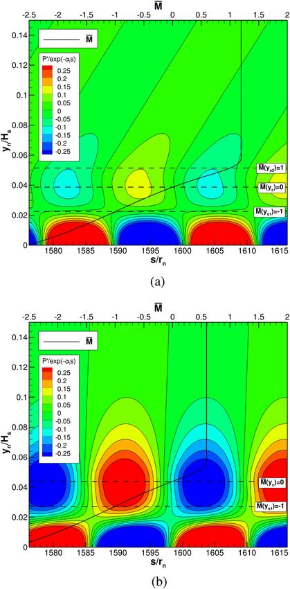
Physics of Fluids                                                                                        ARTICLE             scitation.org/journal/phf

                                                                                        the supersonic mode in the cold wall case and not the other. They rea-
                                                                                        soned that this was due to modal interaction and suggested a com-
                                                                                        bined LST and DNS approach to study the supersonic mode. Zanus
                                                                                        et al.17 revisited the case of Knisely and Zhong using a combination of
                                                                                        LST, linear parabolized stability equations, and DNS. In one warmer
                                                                                        wall case, they found the sound radiation came from a stable super-
                                                                                        sonic mode interacting with the slow acoustic.
                                                                                               Additional theoretical work in the area of supersonic mode insta-
                                                                                        bilities has been done by Wu,18 and Wu and Zhang,19 who studied the
                                                                                        radiation of supersonic beams emanating from wavetrains. The result
                                                                                        is qualitatively similar to the acoustic-like waves seen in unsteady
     FIG. 1. Weak acoustic-like waves emitting from the boundary layer. The waves are   supersonic mode simulations.
     similar in appearance to those emitted by the supersonic mode.                            The present paper shares some commonalities with the literature
                                                                                        already discussed but differs significantly in wall temperature and flow
                                       ðyÞ  c
                                       u                                                enthalpy. To gain a better idea of where the current case lies in the
                                MðyÞ ¼           > 1;                             (1)
                                          a ðyÞ                                        space of supersonic mode investigations, Fig. 2 compares the total free-
                                                                                        stream enthalpy and wall-to-recovery temperature ratio of recent

    where MðyÞ                                   ðyÞ is the steady boundary
                   is the relative Mach number, u                                       investigations with the present investigation. In some instances, the
    layer velocity, c ¼ x=a is the disturbance phase velocity defined by                 freestream enthalpy and temperature ratios had to be calculated from
    circular frequency x and streamwise wavenumber a, and a ðyÞ is the                 available parameters. The general trend in Fig. 2 shows that the most
    local steady flow speed of sound.                                                    recent investigations are highly cooled flows over a range of enthalpies.
          Mack also showed that supersonic modes transfer energy away                   This is because unstable supersonic modes are reliably known to exist
    from the wall. In unsteady simulations, this property is exhibited as               in cooled flows, as Bitter and Shepherd15 put forth. Figure 2 also shows
    acoustic-like emissions from the boundary layer into the flow behind                 that the unstable supersonic mode is not highly dependent on the free-
    the bow shock. In Mack’s 198712 numerical investigation, he found                   stream stagnation enthalpy. Low-enthalpy cases with warmer wall
    unstable supersonic waves—the instability, however, was much weaker                 conditions were included in the studies done by Chuvakhov and
    than the second-mode instability and was thus considered less                       Fedorov,8 and Mortensen.4 However, in both instances, no supersonic
    consequential.                                                                      mode behavior was observed associated with the unstable second
          Recently, there has been a renewed interest in supersonic modes.              mode, and no other modes appear to have been investigated.
    Their presence in high-enthalpy impulse facilities motivated Bitter and                    The current investigation is far removed from the general trend
    Shepherd15 to numerically investigate unstable supersonic modes over                in Fig. 2, making this paper’s in-depth analysis of a low-enthalpy flow
    cold walls with linear stability theory (LST). They found that decreas-             with warm-wall condition unique in the literature. Amongst the recent
    ing the wall-to-edge temperature ratio leads to unstable supersonic
    modes appearing over a broader range of frequencies. Their work also
    characterized an unstable discrete mode (like Mack’s second-mode
    instability) is likely to become supersonically unstable when the com-
    plex phase speed has to cross the slow acoustic continuous spectrum.
          Shortly thereafter, Chuvakhov and Fedorov performed theoreti-
    cal and DNS research on unstable supersonic modes where they stud-
    ied highly cooled plates, with particular attention to the “spontaneous
    radiation of sound.”8 Their theoretical work showed that Mack’s
    second-mode instability radiates acoustic-like waves out of the bound-
    ary layer when synchronized with the slow acoustic continuous spec-
    trum when on a sufficiently cool plate. Tumin also studied the same
    flow conditions and concluded that the acoustic-like waves are not the
    result of nonlinear interactions due to nonparallel flow effects and that
    the boundary layer does have a mechanism for redistributing energy
    to the inviscid layer.16
          The effect of nose bluntness on supersonic modes was recently
    studied by Mortensen.4 Mortensen’s findings show that increasing the
    nose radius promotes supersonic mode instability and increases the
    severity of the instability, eventually dominating over the traditional
    second-mode instability. Knisely and Zhong5,6 also did an extensive
    LST and DNS study of supersonic modes in high-enthalpy flows on
    slender blunt cones with warm and cold walls. A notable result of
    theirs is that, while they could detect unstable supersonic modes with              FIG. 2. Comparison of recent supersonic mode investigations and the present
    DNS in both hot and cold wall cases, LST analysis could only detect                 investigation by freestream enthalpy and recovery temperature ratio.

Phys. Fluids 33, 054104 (2021); doi: 10.1063/5.0048089                                                                                                   33, 054104-2
Published under an exclusive license by AIP Publishing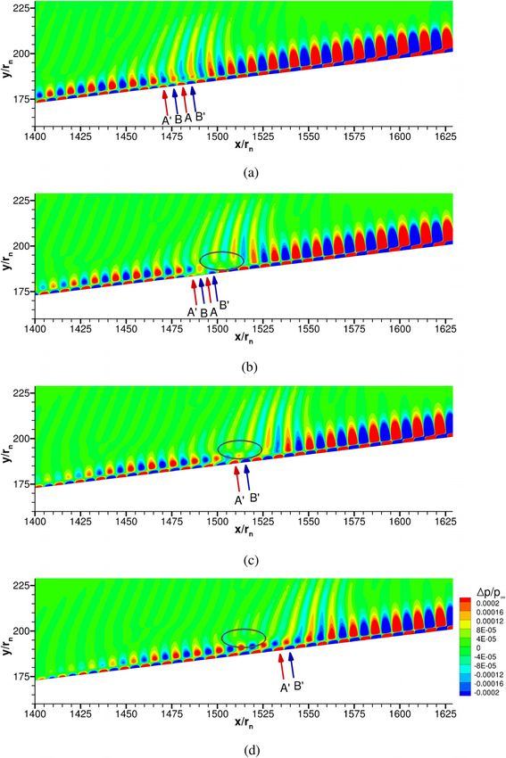
Physics of Fluids                                                                                    ARTICLE            scitation.org/journal/phf

    supersonic mode investigations, the case parameters in this paper               and
    occupy an unexamined space that has been otherwise dismissed
    because the unstable mode did not have supersonic mode attributes,                                                     @T
                                                                                                                 qj ¼ j       :                          (8)
    leaving stable modes unexplored. The current investigation seeks to                                                    @xj
    understand an unexpected numerical result and to shed light on the              Equation (2) is closed assuming a calorically perfect gas
    supersonic mode in low freestream enthalpy flows with a warm-wall
    condition.                                                                                                     p ¼ qRT;                               (9)
          This paper is organized as follows: the governing equations and
    computational methodology are introduced in Sec. II and followed by             which is a reasonable assumption for low-enthalpy hypersonic flows.
    the investigation’s results in Sec. III. This section is divided into several   The properties of nitrogen gas are used, which is consistent with the
    parts between steady-state flow in III B, the LST analysis in Sec. III C,        experimental case from which this simulation takes its parameters.21
    and the results of two unsteady DNS cases in Sec. III D. A brief                The specific heats cp and cv are held constant with a given specific
    description of linear stability theory and relevant details for interpret-      heat ratio of c ¼ 1:4. Meanwhile, a specific gas constant of
    ing the results is provided alongside the LST results in Sec. III C.            R ¼ 296:8 J=kg K for nitrogen gas is used, and the viscosity coefficient,
    Likewise, the unsteady simulation methodology is provided with the              l, is calculated by Sutherland’s law in the form
    DNS results in Sec. III D. The final discussion and conclusion are pro-                                          3=2
                                                                                                                      T      To þ Ts
    vided in Sec. IV.                                                                                       l ¼ lr                   ;                 (10)
                                                                                                                     To       T þ Ts
    II. GOVERNING EQUATIONS AND COMPUTATIONAL
    METHODOLOGY                                                                     where lr ¼ 1:7894  105 N s/m2, To ¼ 288:0 K, and Ts ¼ 110:33 K.
                                                                                    Finally, the Prandtl number is taken as 2=3l and the thermal conduc-
          This paper uses direct numerical simulation (DNS) of the
                                                                                    tivity, j, is computed from the constant Prandtl number
    Navier–Stokes equations to obtain steady and unsteady hypersonic
    flow solutions over a blunt cone. The DNS code utilizes a unique                                                     cp l
                                                                                                                   j¼        :                          (11)
    approach of high-order accurate schemes and shock-fitting to com-                                                    Pr
    pute the bow shock’s location and movement over conical geome-
                                                                                    Fong and Zhong,22 Huang and Zhong,23 and Lei and Zhong24 have
    tries.20 The blunt cone geometry and high-order shock-fitting
                                                                                    used the same formulation or similar formulations for simulating per-
    approach have been validated extensively for accuracy.
                                                                                    fect gas hypersonic flow.
    A. Governing equations
                                                                                    B. Numerical approach
         The DNS code solves the conservation-law form of the three-
                                                                                          A shock-fitting method is used to obtain an accurate shock loca-
    dimensional Navier–Stokes equations in Cartesian coordinates.
                                                                                    tion. The shock-fitting method treats the shock as the upper boundary
    Written in vector form, the governing equations are
                                                                                    of the physical domain by computing the bow shock’s location pro-
                                 @U @Fj @Gj                                         duced by the blunt cone. Equation (2) is solved in a computational
                                   þ   þ    ¼ 0;                             (2)    domain with body-fitted curvilinear coordinates ðn; g; f; sÞ, where n is
                                 @t @xj @xj
                                                                                    in the direction of the cone surface, g is normal to the cone surface, f
    in which U is the state vector of conserved quantities, Fj is the inviscid      is in the azimuthal direction, and s is time. Full transformation details
    flux vectors, and Gj is the viscous flux vector in the jth spatial direction.     can be found in Ref. 20.
    The state and flux vectors are defined as                                               Treating the shock as a domain boundary, the transient shock
                                                                                    movement is solved as an ordinary differential equation (ODE) along-
                            U ¼ fq; qu1 ; qu2 ; qu3 ; egT ;               (3)       side the governing equations. The shock position and speed must be
                                                                        T         obtained in the form Hðn; f; sÞ and Hs ðn; f; sÞ, and solved as inde-
     Fj ¼ quj ; qu1 uj þ pd1j ; qu2 uj þ pd2j ; qu3 uj þ pd3j ; ðe þ pÞuj ;         pendent flow variables alongside the governing equations. This is
                                                                             (4)    accomplished by taking the Rankine–Hugoniot relations, which pro-
                                                                                    vide the flow variable boundary conditions behind the shock, as a
    and
                                                                                    function of U1 and the velocity of the shock front vn. The shock front
                         Gj ¼ f0; s1j ; s2j ; s3j ; sjk uk  qj gT ;         (5)    velocity is determined by a characteristic compatibility equation at the
                                                                                    grid point immediately behind the shock. A complete derivation of H
    where e is internal energy, sij is the viscous stress tensor, and qj is the     and Hs can also be found in Ref. 20.
    heat flux. The internal energy, viscous stress, and heat flux, qj, are                  An explicit 5th -order upwind scheme and an explicit 6th -order
    defined as follows:                                                              central finite-difference scheme are used to discretize the inviscid and
                                                                                  viscous terms of Eq. (2) in the n and g-directions. Second-order deriv-
                                              uk uk
                             e ¼ q cv T þ            ;                      (6)     atives are obtained by applying the schemes twice. Derivatives in the
                                               2
                                                                                    f-direction are computed using Fourier collocation. Finally, 5th -order
                                            !
                                @ui @uj                @uk                          Lax–Friedrichs flux splitting is applied to the inviscid flux terms, and a
                       sij ¼ l        þ        þ dij k     ;                (7)     low storage 3rd-order Runge–Kutta method25 is used to converge the
                                @xj @xi                @xk
                                                                                    steady state and to advance the unsteady solutions.

Phys. Fluids 33, 054104 (2021); doi: 10.1063/5.0048089                                                                                             33, 054104-3
Published under an exclusive license by AIP Publishing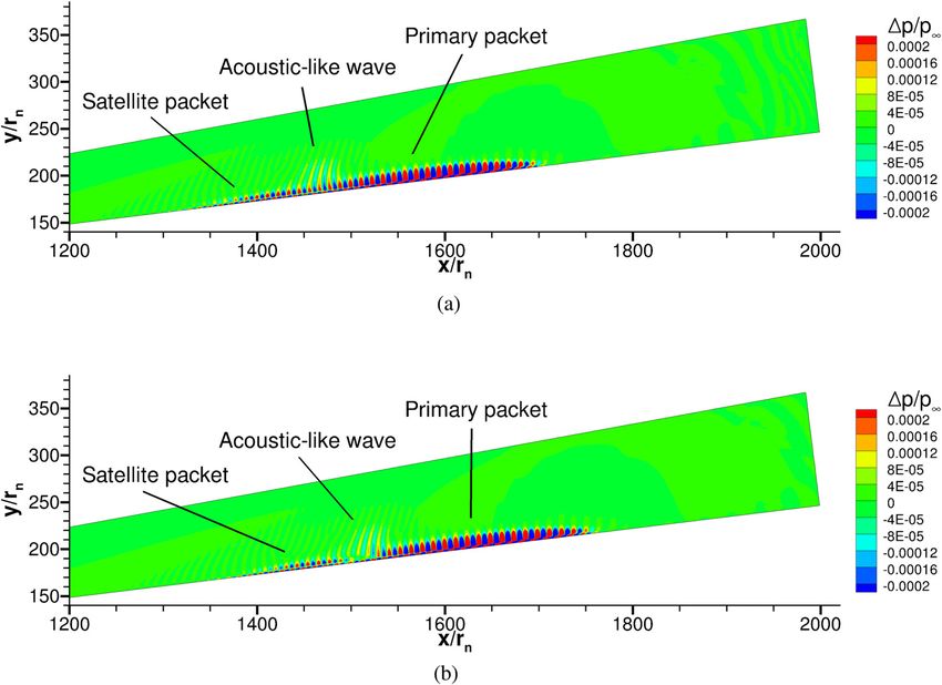
Physics of Fluids                                                                                                ARTICLE               scitation.org/journal/phf

     FIG. 3. Steady-state grid independence study of (a) the velocity boundary layer, and (b) the complex pressure perturbation eigenfunction at s=rn ¼ 500 for wall-normal grid
     distributions J ¼ 121 and 181.

    C. Grid independence and convergence                                                     upstream of the bow shock. The shock-fitting algorithm solves the
          The grid independence study looks at two grid distributions                        flow field behind the shock and determines its steady-state location.
    along the cone frustum: a coarse grid of 3602  121 points and a fine                     An isothermal wall is assumed along the cone surface from the nose
    grid of 7202  181 points. Both grid solutions were converged to a rel-                  tip to the end of the cone. The isothermal boundary condition neglects
    ative pressure error of oðep Þ ¼ 109 . Figure 3(a) plots the velocity                   surface heating by the flow. Moreover, the wall-to-freestream tempera-
    boundary layer at s=rn ¼ 500 for 121 and 181 points in the wall-                         ture ratio in Table I is indicative of a warmer wall.
    normal direction. The profiles are in good agreement for both grid
    point distributions, indicating an independent solution. The accuracy                    B. Steady-state solution
    of the LST stability calculations obtained is also very sensitive to the                      The steady-state pressure and temperature contours for the
    wall-normal grid distribution of the steady state. The pressure eigen-                   cone’s blunt nose and frustum are presented together in Fig. 4.
    function at s=rn ¼ 500 and 160 kHz in Fig. 3(b) also shows there is                      Overall, the steady-state solution is typical for a straight blunt cone.
    good agreement between the two grid point distributions. In summary,                     Looking at the blunt nose tip in Fig. 4(a), the pressure contours show a
    the solution is converged with no significant differences in the bound-                   maximum pressure ratio at the very tip of the cone, followed by a
    ary layer profiles or LST eigenfunctions.                                                 favorable pressure gradient moving downstream. This favorable pres-
    III. RESULTS                                                                             sure gradient quickly gives way to the moderate pressure ratios seen
                                                                                             on the frustum in Fig. 4(b). The temperature contours also show a
         This paper’s simulation approach is to use the aforementioned                       maximum temperature ratio at the nose tip that is offset from the stag-
    shock-fitting code to obtain the steady-state solution around a cone.                     nation point due to the isothermal wall boundary condition. Moving
    The solution is used as the boundary layer profiles for LST analysis                      to the cone’s frustum in Fig. 4(b), the pressure results on the top half
    and as the base flow for unsteady DNS simulations. LST provides a                         of the figure show a moderate pressure ratio and a mildly favorable
    theoretical analysis of the discrete boundary layer modes and provides                   pressure gradient moving downstream along the cone’s length. In the
    the data required to compute modal phase speeds, growth rates, and                       bottom half of Fig. 4(b), the temperature ratio contours show a high
    eigenfunctions. The unsteady DNS simulation provides a time-
    accurate evolution of a boundary layer disturbance, which can be ana-
                                                                                             TABLE I. Freestream flow conditions for DNS simulations.
    lyzed with Fourier decomposition.
                                                                                             Parameter                 Value               Parameter                Value
    A. Simulation conditions
         Specifically, the cone geometry in this paper is a slender straight                  M1                         8.0                  Tw =T1                 6.21

    blunt cone at 0 angle-of-attack with a half-angle of 7 , a nose radius                   q1                  0.024 803 kg/m3             Tw =Tad                0.52
    of 0.5 mm, and a total length of 1.0 m measured from the nose tip.                       p1                     330.743 Pa                 Tw                 279.0 K
    The flow conditions listed in Table I are taken from a previous experi-                   h0;1                  1.174 MJ/kg               Re1 =l            9 584 257 m1
    ment21 performed in Sandia National Laboratories’ HWT-8 for the                          U1                    1093.07 m/s
    same cone geometry. The freestream conditions are assumed fixed

Phys. Fluids 33, 054104 (2021); doi: 10.1063/5.0048089                                                                                                               33, 054104-4
Published under an exclusive license by AIP Publishing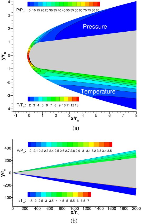
Physics of Fluids ARTICLE scitation.org/journal/phf
from the substitution. Assuming a parallel flow, the remaining steady
terms become a function of y only—in practice, the steady-state solu-
tion is obtained from the DNS solution and is assumed to be locally
parallel. Higher-order fluctuating terms are assumed to be small and
are linearized. Finally, a normal mode solution is assumed for the fluc-
tuations of the form
q0 ðyÞ ¼ ^q ðyÞ exp ½iðax þ bz xtÞ; (12)
0 0 0
where q ðyÞ is the vector of the fluctuating variables fu ðyÞ; v ðyÞ;
p0 ðyÞ; T 0 ðyÞ; w0 ðyÞgT ; ^q ðyÞ is the vector of their complex eigenfunc-
tions, a and b are the wavenumbers, and x is the circular frequency.
Substituting the normal mode solution in for the fluctuating terms
results in a coupled set of five ordinary differential equations
!
d2 d
A 2 þ B þ C ^q ðyÞ ¼ 0; (13)
dy dy
where A, B, and C are complex square matrices and can be found in
Ref. 28. Equation (13) constitutes an eigenvalue problem, wherein
Dirichlet boundary conditions are applied at the surface and in the
far-field. The far-field boundary conditions do not include the bow
shock, which is present in the steady-state shock-fitting simulation.
For the purposes of this investigation, the shock is considered to be
sufficiently far away from the boundary layer as not to have a signifi-
cant effect on the stability calculations.
The resulting eigenvalue problem is then solved using Malik’s
multi-domain spectral method approach and a packaged complex
eigenvalue solver. The solution of which provides the dispersion rela-
tion, X, and the complex eigenfunction vector, ^q .
The LST equations can be solved using either a temporal stability
approach or a spatial stability approach. For the purposes of compari-
son with DNS, a spatial stability approach is used wherein x is real,
the perturbation is assumed to be 2D ðb ¼ 0Þ, and Eq. (13) is solved
for a complex a. The result is a solution to the dispersion relation:
a ¼ XðxÞ.
In this paper, LST is used to obtain the dispersion relations for
FIG. 4. Pressure and temperature contours at the (a) blunt nose tip, and on the (b)
the discrete boundary layer modes F and S at select frequencies. The
cone frustum. The figures are split with pressure ratio plotted on the top half and discrete modes’ phase speed and growth rate are computed from these
temperature ratio plotted on the bottom half. LST results. The nondimensional phase speed is defined as
x
thermal gradient between the boundary layer and the flow behind the cr ¼ ; (14)
ar
shock, extending over the entire frustum. This high thermal gradient is
expected due to the isothermal wall condition, which is considerably where ar is the real part of the nondimensional wave number. The non-
higher than the temperature behind the shock and the freestream dimensional phase speed is used to identify the discrete modes based on
temperature. where they originate amongst the continuous spectra and interpret their
behavior. Likewise, the dimensional growth rate, ai =L , is the negative
of the imaginary part of the complex wavenumber over the boundary
C. Linear stability analysis of steady state pffiffiffiffiffiffiffiffiffiffiffiffiffiffiffiffiffiffiffiffi
layer length scale, L , where L ¼ sl1=q1 U1 and s is the distance
1. Linear stability theory along the cone surface. The growth rate is used to identify stable and
unstable modes: positive growth rates for unstable modes and negative
This paper’s linear stability analysis is conducted with a com- growth rates for stable modes.
pressible LST code developed by Ma26,27 following the work done by
Malik.28 To provide a brief overview of LST theory’s derivation, the
2. Results of linear stability analysis
compressible LST equations are obtained from the governing equa-
tions, wherein an instantaneous solution comprised of a steady term To study the boundary layer’s stability characteristics, LST is
and a fluctuating term is substituted into Eq. (2). The steady part of used with the steady-state solution to obtain the discrete boundary
the flow is assumed to satisfy Eq. (2) independently and is subtracted layer modes F and S. For this particular spatial stability analysis,
Phys. Fluids 33, 054104 (2021); doi: 10.1063/5.0048089 33, 054104-5
Published under an exclusive license by AIP Publishing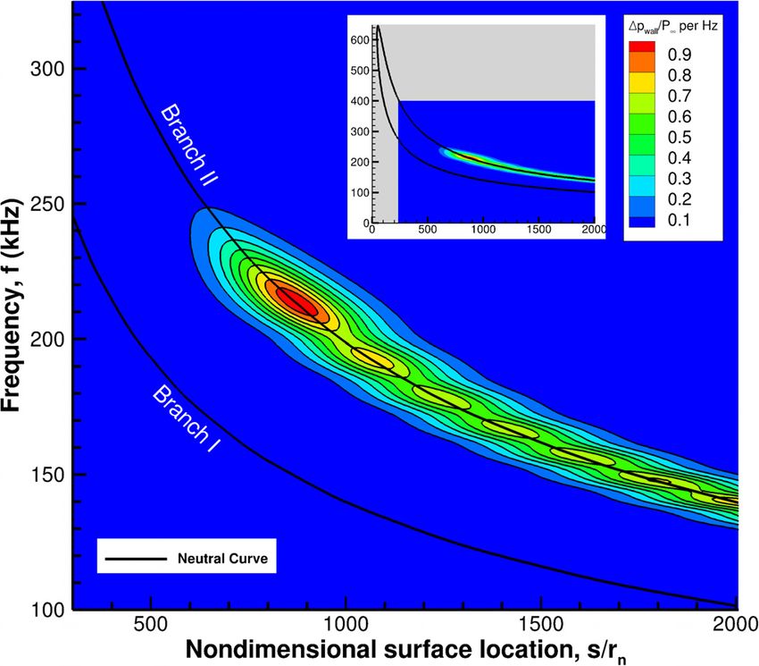
Physics of Fluids                                                                               ARTICLE            scitation.org/journal/phf

    160 kHz and 260 kHz are chosen as representative frequencies. As will      boundary layer (see Fig. 9 of Ref. 6 and Figs. 14 and 15 of Ref. 8).
    be seen in Sec. III D, 160 kHz is close to where the constructive/         Moreover, the unstable supersonic mode F1 had to cross the slow
    destructive interference behavior occurs, and 260 kHz is in the vicinity   acoustic continuous spectrum branch cut, resulting in a bifurcation of
    of blowing-suction actuators.                                              the mode (see Fig. 16 of Ref. 5 and Fig. 4(a) of Ref. 8). There is no sim-
          Before proceeding, a small discussion on discrete mode terminol-     ilar bifurcation of mode F1 in the present study since its stability
    ogy is in order. In general, this paper follows the modal naming con-      keeps it away from the slow acoustic continuous spectrum branch cut
    ventions put forth by Fedorov and Tumin.29 Mode F describes the            as seen in Fig. 6. Thus, any acoustic-like waves produced by the super-
    discrete modes that originate from the fast acoustic spectrum where        sonic mode F1 are likely to be damped.
    cr ¼ 1 þ 1=M1 , and mode S describes the discrete mode that origi-               In addition to the LST results, Figs. 5(a) and 5(b) contain phase
    nates from the slow acoustic spectrum where cr ¼ 1  1=M1 . If more        speed and growth rate results obtained from DNS. The complex wave-
    than one discrete mode appears from either acoustic spectrum, the          number components needed to compute the phase speed and growth
    modes are numbered in order of appearance by increasing x.                 rate are obtained from the amplitude and phase angle of the Fourier
    Occasionally, a discrete mode may undergo a branch cut or bifurcation      decomposed pressure fluctuations at the wall. The wavenumber’s real
    when crossing one of the continuous spectra, such as the entropy/          and imaginary parts are computed using the following equations:
    vorticity spectrum (cr ¼ 1). In such a case, as x is increased, the mode
                                                                                                                d
    approaching the branch cut is given a “þ,” and the mode departing                                       ar ¼  wðf Þ;                            (15)
    the branch cut is given a “.” In this paper, mode F undergoes a                                           ds
    branch cut when crossing the entropy/vorticity spectrum. In Refs. 5,                                       1 d
                                                                                                      ai ¼            D/ðf Þ;                      (16)
    15, and 16, however, mode F both crosses a branch cut and bifurcates                                     D/ðf Þ ds
    when crossing the entropy/vorticity spectrum and slow acoustic spec-       where D/ðf Þ is the pressure amplitude-frequency at the wall, and
    trum, respectively, and “þ/” usage is redefined. These references and      wðf Þ is the phase angle at frequency f. The resulting phase speed and
    this paper use very similar but incongruous discrete mode terminol-        growth rate results consist of the combined discrete and continuous
    ogy, so it is important to note that identically named modes may not       modes. Bi-orthogonal decomposition can be used to extract the dis-
    describe the same physical mode.                                           crete modes from the combined signal,30 but the decomposition is out
          The phase speed and growth rate of modes F and S at 160 kHz          of scope of the current research. In the meantime, it is possible to gain
    and 260 kHz are featured in Fig. 5. Figure 5(a) and 5(c) shows how         some insight and comparison between LST and DNS without decom-
    mode F1þ originates in the fast acoustic spectrum and steadily slows       posing the signal further, assuming that the more dominant mode has
    down until it reaches the vorticity/entropy branch cut where F1           a more significant influence on the combined signal.
    emerges on the other side. As mode F1’s phase speed continues to                The large oscillations seen in the DNS results in both Figs. 5(a)
    decrease, it couples with mode S, as seen by the mirrored modal            and 5(b) around x ¼ 0:15 are attributed to the proximity of the dis-
    growth rate curves in Figs. 5(b) and 5(d). After coupling, mode F1        turbance to the actuator and are attributed to forcing. In general, the
    slows to the slow acoustic wave speed and passes it without coalescing     DNS phase speed in Fig. 5(a) follows the LST result for mode S; how-
    or bifurcating with the slow acoustic branch cut.                          ever, it appears translated downward slightly, which could be attrib-
          Conversely, mode S originates from the slow acoustic spectrum        uted to influences by mode F1. It is also important to note that the
    and takes on a phase speed between cr ¼ 1 and cr ¼ 1  1=M1 . The          phase speed dips below cr < 1  1=M1 around x ¼ 0:255, indicat-
    coupling of mode F1 and mode S causes mode S to become unstable.          ing the phase speed becomes supersonic. This supports the idea that
    This is the well-known second-mode instability and is the only unsta-      the acoustic-like waves seen Fig. 1 and in the unsteady results in Sec.
    ble mode found in the LST analysis. Furthermore, mode F1 is stable        III D result from a supersonic mode. The DNS growth rate in Fig. 5(b)
    as a consequence of coupling.                                              also follows, albeit slightly below, the LST result for mode S, before
          Of primary interest to the paper is when any discrete modes          trending toward the stable growth rate for mode F1. The DNS phase
    become supersonic. This is because the acoustic-like waves seen in         speed and growth rate trends agree reasonably well with the LST
    Fig. 1 are indicative of a supersonic mode. In addition to the super-      results. The DNS results also support the presence of a supersonic
    sonic region within the boundary layer, where M   < 1, there is a sec-   mode.
    ond region of relative supersonic flow above it where M    > 1. In order         To better understand how discrete modes can interact with the
    for M to be greater than one, the nondimensional phase speed must         continuous spectra, the discrete modes featured in Fig. 5 are plotted
    be less than 1  1=M1 . Thus, a discrete mode will be supersonic           with the continuous spectra branch cuts in the complex phase speed
    when cr < 1  1=M1 .                                                       plane in Fig. 6. The mode’s complex phase speed is computed by
          Of the modes in Fig. 5, only mode F1 is slower than the slow        dividing the mode’s frequency by its complex wave number. The real
    acoustic and becomes supersonic at x ¼ 0:23. When the phase speed          part of the complex phase speed is plotted along the x axis and the
    of a discrete mode is supersonic, it is possible for acoustic-like waves   imaginary part along the y axis. Demarcations along the top of Fig. 6
    to emit into the inviscid region outside of the boundary layer.            denote where discrete modes become supersonic and subsonic based
    However, mode F1 is very stable, and any acoustic-like waves are          on their nondimensional phase speed. Likewise, divisions along the
    likely to be weak and not sustained without forcing.                       right side denote where the discrete modes become stable and unsta-
          By contrast, the supersonic mode in Knisley and Zhong5,6 and         ble. In addition to the discrete modes, the figure also includes the
    Chuvakhov and Fedorov8 was an attribute of an unstable F1 mode.            branch cuts for the fast acoustic, vorticity/entropy, and slow acoustic
    Because the mode was unstable, they saw very a strong supersonic           continuous spectra. The branch cut locations are calculated using the
    response with acoustic-like waves propagating farther outside the          methods developed by Balakumar and Malik.31

Phys. Fluids 33, 054104 (2021); doi: 10.1063/5.0048089                                                                                        33, 054104-6
Published under an exclusive license by AIP Publishing
Physics of Fluids                                                                                                ARTICLE              scitation.org/journal/phf

     FIG. 5. Nondimensional (a) phase speed and (b) growth rate results for discrete modes F and S at 160 kHz and (c) and (d) 260 kHz, respectively. 160 kHz frequency includes
     phase speed and growth rate results obtained from unsteady DNS.

          Concerning the discrete modes, Fig. 6 shows F1þ originating near                         Similar complex phase speed figures have been plotted by
    the fast acoustic spectrum branch cut on the right side of the figure and                 Refs. 8, 9, 15, and 16 in their supersonic mode investigations (see Figs.
    then moving left to the vorticity/entropy spectrum branch cut with                       4, 16, 10, and 4 of Refs. 8, 9, 15, and 16, respectively). In those investi-
    increasing x where it stops. From the other side of the vorticity/entropy                gations, the emergence of a separate discrete supersonic mode was
    spectrum branch cut, mode F1 emerges and moves to the left with                         synonymous with a discrete mode coalescing with the slow acoustic
    increasing x, at one point crossing from a subsonic to supersonic phase                  spectrum branch cut from above and a separate discrete supersonic
    speed. Note that both F1þ and F1 are in the stable region of Fig. 6.                    mode emerging from below. Thus, the coalescing discrete mode had
    Mode S originates from the bottom of the figure near the slow acoustic                    to have a phase velocity less than 1  1=M1 , and an imaginary phase
    phase speed line and moves upwards toward the unstable region with                       velocity greater than the slow acoustic branch cut, meaning it was
    increasing x before looping back to the stable region. Unlike mode F,                    both supersonic and unstable. For visual reference, this puts the mode
    mode S is confined to the subsonic phase speed region.                                    in the upper-left region of Fig. 6. None of the discrete modes

Phys. Fluids 33, 054104 (2021); doi: 10.1063/5.0048089                                                                                                              33, 054104-7
Published under an exclusive license by AIP Publishing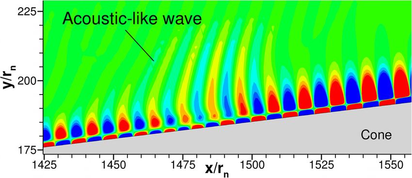
Physics of Fluids                                                                                        ARTICLE             scitation.org/journal/phf

     FIG. 6. Discrete modes F and S in the complex phase speed plane for f ¼ 160 and
     260 kHz.

    investigated by this paper appear in the phase speed plane’s upper-left
    region. LST predicts that the supersonic mode behavior seen in this
    paper does not appear to result from coalescing or emerging discrete
    modes. Instead, it results from a stable mode F1’s decreasing phase
    speed. By contrast, the coalescing discrete mode in the literature cited
    above was an unstable mode F1 (according to this paper’s mode
    naming convention). The cited literature also had a very strong
    acoustic-like wave response, likely due to the mode’s instability.
    However, this is not the case here, where the mode’s stability makes
    the acoustic-like wave response comparatively weak, as seen in the
    propagating disturbance in Fig. 10. To summarize, the supersonic
    mode F1 observed in this paper lacks the instability and coalescence
    with the slow acoustic spectrum branch cut seen in the investigations
    mentioned above. These differences provide a new view of how super-
    sonic discrete modes behave in low-enthalpy flows with warm-wall
    conditions.
          Moreover, the unstable mode S does not appear to play a role in
    the observed supersonic behavior unlike the unstable mode in the
    investigations mentioned above. The loop seen in Fig. 6 is because
    mode S is multi-valued in cr due to coupling with F1 (which is
                                                                                       FIG. 7. Comparison of (a) mode F1 and (b) mode S pressure eigenfunctions at
    monotonic in cr). Moreover, since mode S generally increases in cr                 x ¼ 0:23, after synchronization and in the vicinity of the slow acoustic phase
    with increasing x, it is not likely to cross the slow acoustic wave speed          speed.
    and is therefore not susceptible to supersonic behavior.
          Further insight into modes F and S’s behavior can be gained by               accounting for the growth in the boundary layer and grid stretching in
    examining the real part of their pressure eigenfunction. In Ref. 5, the            the wall normal direction introduced by normalizing the vertical coor-
    supersonic mode’s eigenfunction has a strong oscillatory feature that              dinate, yn, by the shock height, Hs. The boundary layer edge d99 =Hs is
    extends outside of the boundary layer. To investigate similar features,            denoted by red x’s in each plot; for both mode F1 and mode S, the
    this study looks at both mode F1 and S before and after mode F1’s                eigenfunction extends above the boundary layer and does not deviate
    phase speed crosses the slow acoustic wave speed. Figure 7 contains                away from ^p r ¼ 0 once reaching that value in the inviscid layer. Since
    the eigenfunctions at x ¼ 0:23, right before mode F1 becomes                      x ¼ 0:23 is just before mode F1 becomes supersonic, oscillations
    supersonic, for both modes F1 and S at 160 and 260 kHz. In general,               into the area behind the shock are not expected for either discrete
    the eigenfunctions’ shapes are very similar for both frequencies when              mode.

Phys. Fluids 33, 054104 (2021); doi: 10.1063/5.0048089                                                                                                    33, 054104-8
Published under an exclusive license by AIP Publishing
Physics of Fluids                                                                                       ARTICLE             scitation.org/journal/phf

         Continuing downstream to x ¼ 0:26 where mode F1’s phase                    stretching. As before, the profiles extend above the boundary layer
    speed is now supersonic, Fig. 8 contains the plots of the real part of the       edge; however, their shape is slightly different from that seen at
    pressure eigenfunction for both discrete modes at the same frequencies           x ¼ 0:23. The mode S profiles are similar, as they do not move away
    as before. While mode F1’s phase speed is supersonic, mode S’s                  from ^p r ¼ 0 in the inviscid layer. However, the profiles for mode F1
    phase speed is not, thus any oscillations beyond the boundary layer are          oscillate once about ^p r ¼ 0 above the boundary layer edge before
    expected to appear for mode F1 and not mode S. The eigenfunctions               returning to zero, as seen in the inset plot of Fig. 8(a). This oscillation,
    are again similar across frequency when controlling for vertical                 although weak, is significant because it provides a mechanism for
                                                                                     acoustic-like waves to appear in the flow behind the shock. Similarly,
                                                                                     unstable supersonic modes produce more persistent oscillations
                                                                                     beyond the boundary layer edge (see Fig. 15 of Ref. 5), resulting in the
                                                                                     acoustic-like waves seen in the inviscid layer. Furthermore, mode S
                                                                                     does not exhibit any oscillations on account of its subsonic phase
                                                                                     speed. Thus, it is reasonable to conclude that since mode F1’s eigen-
                                                                                     function has no oscillations when subsonic and a weak oscillation
                                                                                     when supersonic that mode F1 is responsible for the acoustic-like
                                                                                     waves seen in the DNS results.
                                                                                           An effective way to visualize the supersonic mode using the LST
                                                                                     framework is to expand the pressure eigenfunction to produce a con-
                                                                                     tour plot of the pressure fluctuations. An approximate 2D representa-
                                                                                     tion of the discrete modes can be obtained using the real part of the
                                                                                     normal mode equation used to derive the LST equation

                                                                                                            p0 ðyÞ ¼ Ref^p ðyÞeðiðasxtÞÞ g;                  (17)
                                                                                     which simplifies to

                                                                                        p0 ðyÞ ¼ ^p r ðyÞ cosðar s  xtÞ  ^p i ðyÞ sinðar s  xtÞ eai s :   (18)
                                                                                     By substituting the pressure eigenfunction, ^p , into Eq. (18), along with
                                                                                     its wavenumber, a, and frequency, x, the pressure perturbation, p0 ,
                                                                                     can be obtained at its streamwise location, s. A contour plot of the per-
                                                                                     turbation is then generated by varying s slightly upstream and down-
                                                                                     stream, as seen in Fig. 9. The contour levels are normalized by the
                                                                                     growth rate term eai s and clipped to visualize the mode better.
                                                                                           The resulting contour plots in Fig. 9 are the normalized pressure
                                                                                     fluctuations for modes F1 and S at 160 kHz and x ¼ 0:26. The local
                                                                                     relative Mach number, computed with respect to its discrete mode’s
                                                                                     phase speed, is plotted on top of the pressure fluctuations as a function
                                                                                     of boundary layer height. Dashed lines in each figure demark relative
                                                                                     Mach numbers of interest, such as the first sonic line (Mðy  s1 Þ ¼ 1),
                                                                                                          c Þ ¼ 0), and the second sonic line (Mðy
                                                                                     the critical layer (Mðy                                       s2 Þ ¼ 1).
                                                                                     The dashed lines also effectively denote regions in the boundary layer
                                                                                     where the relative Mach number is subsonic (1 < MðyÞÞ          < 1) and

                                                                                     supersonic (MðyÞ > 1 and MðyÞ < 1).
                                                                                           The pressure fluctuation for mode F1 in Fig. 9(a) produces a
                                                                                     unique asymmetric repeating pattern. The small oscillation seen in the
                                                                                     real part of the eigenfunction in Fig. 8(a), when paired with its imagi-
                                                                                     nary component, actually reveals decaying Mach waves. These Mach
                                                                                     waves have a similar appearance to the acoustic-like waves emanating
                                                                                     from the boundary layer seen in Fig. 1, albeit smaller in size. Most
                                                                                     importantly, these Mach waves also appear above the second sonic
                                                                                     line where the relative Mach number is supersonic. When the relative
                                                                                     Mach number is greater than 1, the flow is supersonic with respect to
                                                                                     the mode’s phase speed, signifying that the mode is propagating
                                                                                     upstream supersonically in the flow’s inertial frame; this is why the
     FIG. 8. Comparison of (a) mode F1 and (b) mode S pressure eigenfunctions at    Mach waves are angled downstream. Moreover, the Mach waves and
     x ¼ 0:26, downstream where mode F1’s phase speed is less than that of a slow   second sonic line are consistent with the supersonic mode diagram
     acoustic wave.                                                                  prepared by Knisely and Zhong for a neutral supersonic mode in the

Phys. Fluids 33, 054104 (2021); doi: 10.1063/5.0048089                                                                                                   33, 054104-9
Published under an exclusive license by AIP Publishing
Physics of Fluids ARTICLE scitation.org/journal/phf
waves and has no second sonic line. The absence of these two features
is expected because, as shown in Fig. 5(a), mode S is subsonic at
x ¼ 0:26. The relative Mach number profile in Fig. 9(b) confirms this
because at no point in the boundary layer is the relative Mach number
greater than 1. This is because mode S has a faster wave speed relative
to the meanflow than mode F1. As such, mode S cannot produce
Mach waves. Therefore, any supersonic mode behavior observed in
the DNS results is due to mode F1 and not mode S.
To summarize, the LST analysis for mode F1 shows that it
takes on a supersonic phase speed downstream and has an upper sonic
line in the boundary layer when supersonic, and that its eigenfunction
produces acoustic-like waves. Therefore, if there exists a supersonic
mode in the unsteady simulation, it is likely the result of mode F1.
Similarly, mode S is expected to be subsonic and unstable and not
responsible for the observed supersonic behavior.
D. DNS results on a smooth cone
Two unsteady cases are considered in this paper that differ only
in the blowing-suction actuator’s location. In Case I, the actuator is
located at the surface location, sc =rn ¼ 400, measured from the nose
tip, and in Case II at sc =rn ¼ 200. Initially, the appearance of the pri-
mary and satellite waves and acoustic-like waves was observed in Case
I. Since the appearance of the acoustic-like waves was unexpected for
the present flow conditions, Case II was run to investigate whether the
actuator’s location was a cause for the unexpected result. The same
steady base flow and pulse parameters are used for both DNS cases.
1. Simulation of disturbance
Unsteady disturbances are simulated using a blowing-suction
actuator on the cone surface to introduce an unsteady pulse into the
steady-state solution flow field. The actuator extends circumferentially
around the cone. The pulse has a Gaussian distribution in time and is
sinusoidal in space. The sinusoidal shape prevents introducing addi-
tional mass into the simulation. The frequency spectrum of the pulse
is broad enough to include the most unstable mode frequencies for the
given flow conditions. Downstream of the actuator, each frequency is
examined for amplification or attenuation based on the frequency
spectrum of a temporal Fourier decomposition (FFT). Normalizing
each frequency by its initial amplitude makes it possible to compare
growth and decay across all frequencies.
The technique of using a Gaussian pulse to examine mode ampli-
fication/attenuation was previously implemented by Fong and
Zhong32 and Knisely and Zhong.5,6 The blowing-suction actuator’s
mass flux follows the equation:
FIG. 9. Normalized pressure fluctuation contours for (a) mode F1 and (b) mode
S overlaid with local relative Mach number. Contours are constructed from pressure ðt lÞ2 s sc
_ p ðs; tÞ ¼ eðqUÞ1 exp
m sin 2p ; (19)
eigenfunction results obtained from LST at 160 kHz and x ¼ 0:26. The locations of 2r2 l
the first (ys2 ) and second (ys1 ) sonic lines and critical layer (yc) are demarcated by
relative Mach number. for sc < s < sc þ l and t > 0. In which l is the mean, r is the stan-
dard deviation, sc is the actuator’s surface location, and l is the length
large wave number limit (see Fig. 2 in Ref. 5). Thus, the appearance of of the actuator. The mass flux is scaled by eðqUÞ1 , where imposing a
Mach waves above the second sonic line provides further justification small e keeps the flow field’s response linear and prevents nonlinear
that mode F1 is the supersonic mode responsible for the acoustic- interaction between different frequencies. In this way, the pulse distur-
like waves. bance can be decomposed, and each frequency can be studied inde-
Unlike mode F1, the contour of mode S in Fig. 9(b) produces a pendently. The mean of the pulse, l, is defined in terms of a
symmetric repeating pattern of perturbations without decaying Mach minimum mass flux, ðqvÞmin , the initial mass flux at t ¼ 0,
Phys. Fluids 33, 054104 (2021); doi: 10.1063/5.0048089 33, 054104-10
Published under an exclusive license by AIP PublishingPhysics of Fluids ARTICLE scitation.org/journal/phf
TABLE II. Gaussian pulse parameters for DNS. in Fig. 13, the two portions of the disturbance consist of a primary and
satellite wave packet. This brings us to another peculiar aspect of this
Parameter e ðqvÞmin (kg m/s) r (ls) l (ls) xs (m) l (mm) unsteady disturbance: the periodic constructive/destructive interfer-
ence between these two packets. As seen in Fig. 10(b), destructive
Value 103 1010 0.3 2.0398 0.1976 1.9703
interference creates a “hole” in the oscillation beneath the acoustic-like
waves. The hole originates near the surface and does not propagate
vffiffiffiffiffiffiffiffiffiffiffiffiffiffiffiffiffiffiffiffiffiffiffiffiffiffiffiffiffiffiffiffiffiffiffiffiffi
!ffi with the pulse, eventually exiting the disturbance altogether as it prop-
u
u ðqvÞ agates downstream. A more detailed look at the interference phenom-
l ¼ t2r2 ln min
: (20) enon is described in Fig. 11.
eðqUÞ1
The acoustic-like wave emissions and constructive/destructive
By defining l in this way, it can be fixed with a reasonable ðqvÞmin interference are evident in Fig. 11(a). The downstream angle of the
regardless of the simulation conditions. The only remaining free emissions is indicative of their supersonic phase speed as they are
parameter in Eq. (19) is the standard deviation, r, which permits direct propagating supersonically upstream relative to the base flow (albeit
control over the pulse’s frequency content. The standard deviation in translating downstream with the disturbance). The emissions, how-
Table II produces a pulse with a nominal spectrum greater than ever, are very weak compared to the much stronger primary wave to
1 MHz, which is sufficient for the range of unstable mode frequencies its right and the satellite wave to its left. Figure 11(a) shows the distur-
found in the unsteady simulation. The remaining pulse parameters bance’s initial state before any wave interference occurs. In Fig. 11(b),
used in this paper are given in Table II. oscillations below the first sonic line, denoted by the arrows A and B,
weaken in strength as they start to cancel. Above the first sonic line,
the oscillations around x=rn ¼ 1500–1510 begin to interfere, creating
2. Case I: Upstream actuator location
a hole with no pressure oscillations. By Fig. 11(c), the weakening oscil-
Case I contains the unsteady results that motivated this investiga- lations below the sonic line, A and B, have canceled out completely,
tion: the acoustic-like waves emanating from a traveling disturbance. leaving the oscillations originally to their right and left, A’ and B’, adja-
Figure 10 shows acoustic-like waves emanating from the boundary cent to one another. Moreover, the hole appears to exit the disturbance
layer as the disturbance develops features of the supersonic mode as it and merge with the disturbance-free pressure field. By Fig. 11(d), the
propagates downstream. The acoustic-like waves are relatively weak pulse assumes the same appearance as it did in Fig. 11(a) before the
compared to the overall disturbance strength and do not extend very wave interference began. In total, the interference pattern appears six
far into the flow field behind the shock. However, they resemble the times along the cone’s length, as the acoustic-like waves emanate unin-
supersonic mode and are inconsistent with a pure second-mode insta- terrupted from the disturbance.
bility. The acoustic-like waves are also positioned between a down- One way to view the propagation of the disturbance is to plot it
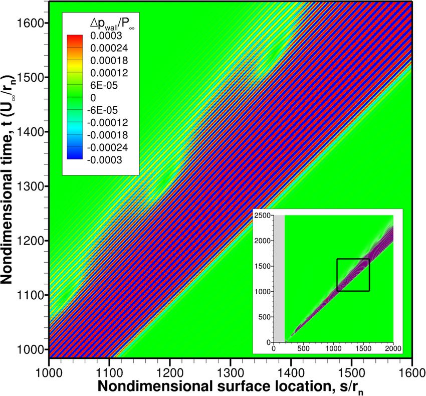
stream and an upstream portion of the disturbance. As will be shown as an x-t diagram, such as in Fig. 12, which shows the pressure
FIG. 10. (a) The acoustic-like waves seen
in context of the entire disturbance. (b) A
hole in the oscillations develops in the
boundary layer beneath the acoustic-like
waves due to the destructive interference
between the primary and satellite wave
packets. The contour levels are clipped to
make the pressure perturbations more
visible.
Phys. Fluids 33, 054104 (2021); doi: 10.1063/5.0048089 33, 054104-11
Published under an exclusive license by AIP PublishingPhysics of Fluids ARTICLE scitation.org/journal/phf
FIG. 12. Case I x-t diagram of unsteady pulse showing the individual wave
trajectories. Contours are clipped to show weaker satellite wave; max
jDpwall =P1 j ¼ 0:0291.
trajectories. In contrast, the satellite wave packet, which appears just
before the first interference patch, comprises slower, steeper trajecto-
ries. As a result of the slower trajectories, the relative Mach number
increases across the disturbance from the primary to satellite wave.
This is noteworthy because if the relative Mach number across the dis-
turbance becomes greater than one, given appropriate values for flow
velocity and speed of sound within the boundary layer, it is possible
for the supersonic mode to exist.
Although the x-t diagram provides an entire overview of the
FIG. 11. Progression of pulse interference patterns: (a) wave train prior to interfer- unsteady disturbance, it is difficult to discern the disturbance’s struc-
ence, (b) interference between oscillations becomes apparent above (ellipse) and ture. Figure 13 features time traces along the surface taken at regular
below (arrows) the first sonic line, (c) above the sonic line a hole in the oscillations nondimensional time intervals, where t has been nondimensionalized
persists into the shock layer, below the sonic line surface oscillations cancel out by the ratio of the freestream velocity to nose radius, U1 =rn . At
(arrows A and B), and (d) wave train returns to its previous appearance. t ¼ 328, the disturbance appears as a single wave packet—this is typi-
cal of previous unsteady simulations containing supersonic modes
perturbation along the cone’s surface over time. An inset plot features after the actuator’s initial forcing.5 Between t ¼ 328 and 682, the dis-
the entire unsteady simulation starting from the actuator location at turbance nearly doubles in amplitude. Growth of the disturbance is
sc =rn ¼ 400, while the enlarged view features the wave trajectories of expected because, as the LST analysis shows, and mode S is unstable.
the disturbance and several instances of constructive/destructive inter- However, its sudden attenuation by t ¼ 1038 is atypical and will be
ference on the cone surface. discussed at the end of this section. By t ¼ 682, however, a satellite
The x-t diagram makes it possible to view the individual wave tra- wave packet appears as a lower amplitude tail on the main packet. In
jectories that makeup the disturbance. From Fig. 12, the leading wave general, the satellite wave packet can be identified as the packet fol-
trajectory that comprises the wavefront is present and consistently the lowing the primary wave and by its lower amplitude. When undergo-
same throughout the unsteady simulation—that is, no new wave trajec- ing destructive interference, the two wave packets appear separate
tories appear ahead of it as time progresses, meaning the wavefront from one another; otherwise, the satellite wave packet appears as a
propagates steadily downstream. However, the trailing wave trajectory is long tail connected to the primary wave packet. By t ¼ 1038, the satel-
not the same throughout the simulation. As time progresses, slower lite wave packet is fully formed, although it is considerably weaker,
wave trajectories appear behind the trailing trajectory, thus becoming with maxjDpwall =P1 j ¼ 1:33 103 compared to the primary waves
the new trailing trajectory and adding to the disturbance’s overall width. at 1:66 102 . For the intervals between t ¼ 1038 and 1749, the sat-
Figure 12 shows that as the wave trajectories fan out from the ellite wave packet is clearly present and separate from the primary
actuator, the primary wave packet comprises the faster shallower wave.
Phys. Fluids 33, 054104 (2021); doi: 10.1063/5.0048089 33, 054104-12
Published under an exclusive license by AIP PublishingPhysics of Fluids ARTICLE scitation.org/journal/phf
FIG. 13. Propagation of disturbance along the cone surface for Case I with actuator FIG. 14. Case I primary and satellite waves packet evolution over a select time
located at sc =rn ¼ 400. The instantaneous pressure is plotted at five equal nondi- interval. At t ¼ 984 and 1202, both wave packets are distinct from one another due
mensional time intervals of 356. to interference between packets. All other instances show the satellite wave packet
as a tail on the primary wave packet. Actuator located at sc =rn ¼ 400.
A closer look at the interference between the primary and satellite
waves is examined in Fig. 14. Whereas Fig. 13 shows the instantaneous Since the disturbance is comprised of many different waves, it is
propagation of the disturbance over most of the cone, Fig. 14 shows in possible to use Fourier decomposition to obtain its frequency spec-
detail the evolution of the primary and satellite wave packets over a trum. The decomposition is important because it provides insight into
shorter interval. The interval from t ¼ 874 and 1312 includes the sec- the growth and decay of individual frequencies and is more readily
ond and third patches seen in the inset plot of Fig. 12. The satellite compared with LST results. The unsteady wall pressure data featured
wave packet is clearly visible and separate from the primary wave in Fig. 12 are used to obtain the disturbance’s frequency spectrum.
packet at t ¼ 984 and 1202, whereas, at t ¼ 874, 1093, and 1312, the The resulting spectrum is normalized by the initial Gaussian pulse in
satellite wave appears as a tail on the primary wave packet. order to compare the growth and decay of individual frequencies
As the disturbance propagates downstream, it spreads in length together, irrespective of their initial strength. The resulting normalized
due to wave dispersion, as seen in Fig. 12. Since the primary and satel- frequency spectrum is featured in Fig. 15 along with the neutral stabil-
lite wave packets are also dispersive, any spreading of the wave packets ity curve for mode S, obtained from LST analysis. There is really good
will cause the waves to interact with one another resulting in either agreement between the spectrum and branch II of the neutral curve.
constructive or destructive interference. Constructive and destructive Since growth rates are unstable between branch I and branch II, and
interference occurs when the superposition of two waves forms a stable everywhere else, amplitudes are expected to grow inside the neu-
resultant wave of greater or lower amplitude. The patches in Fig. 12 tral stability curve and decay outside of it. As Fig. 15 shows, the ampli-
and the holes seen in Fig. 11 are likely caused by destructive interfer- tude grows to the left of the branch II neutral stability curve for a fixed
ence. Likewise, what causes the primary wave and satellite wave to frequency and begins to dampen immediately to the right as expected.
appear attached at t ¼ 874, 1093, and 1312 in Fig. 14 results from con- This result is notable because it shows good agreement between two
structive interference. As was specified previously, the actuator pulse is separate and distinct methods: Fourier decomposition and LST
kept intentionally weak to maintain the disturbance’s linear growth analysis.
and is therefore unlikely to exhibit nonlinear behavior. As such, super- An important feature of Fig. 15 is its notable array of peaks and
position is a linear process that can account for the repeating pattern saddles along the perturbed spectrum aligning with the branch II neu-
of constructive/destructive interference. tral curve. To investigate these peaks and saddles further, fixed fre-
How the primary and satellite wave packets relate to the acoustic- quency slices of the spectrum are plotted in Fig. 16, corresponding to
like waves is unclear at this point. Except to say that the wave packets three pairs of peaks and saddles along the perturbed spectrum. Despite
are probably the result of forcing by the actuator and that the acoustic- the undulations in the frequency spectrum, each frequency still grows
like emissions appear at the interface between primary and satellite and decays in the expected manner—in that there is no modulation
wave packets, as seen in Fig. 11. within a fixed frequency, only a single peak, indicating that the
Phys. Fluids 33, 054104 (2021); doi: 10.1063/5.0048089 33, 054104-13
Published under an exclusive license by AIP PublishingYou can also read