Extracting and Retargeting Color Mappings from Bitmap Images of Visualizations
←
→
Page content transcription
If your browser does not render page correctly, please read the page content below
Extracting and Retargeting Color Mappings
from Bitmap Images of Visualizations
Jorge Poco, Angela Mayhua, and Jeffrey Heer
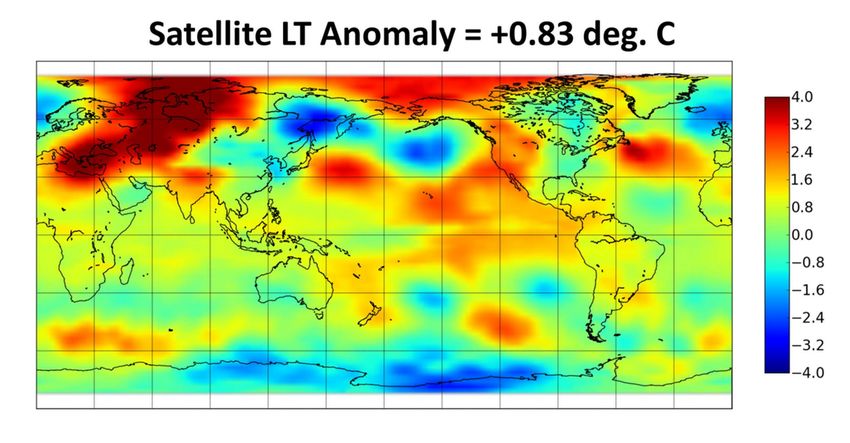
Fig. 1. Automatic extraction and redesign of color mappings for a geographic heatmap. The bitmap image on the left uses a questionable
rainbow color palette. Our methods automatically recover the color mapping, enabling applications such as automatic recoloring. The
generated image on the right replaces the original color palette with a perceptually-motivated diverging color scheme.
Abstract— Visualization designers regularly use color to encode quantitative or categorical data. However, visualizations “in the wild”
often violate perceptual color design principles and may only be available as bitmap images. In this work, we contribute a method
to semi-automatically extract color encodings from a bitmap visualization image. Given an image and a legend location, we classify
the legend as describing either a discrete or continuous color encoding, identify the colors used, and extract legend text using OCR
methods. We then combine this information to recover the specific color mapping. Users can also correct interpretation errors using an
annotation interface. We evaluate our techniques using a corpus of images extracted from scientific papers and demonstrate accurate
automatic inference of color mappings across a variety of chart types. In addition, we present two applications of our method: automatic
recoloring to improve perceptual effectiveness, and interactive overlays to enable improved reading of static visualizations.
Index Terms—Visualization, color, chart understanding, information extraction, redesign, computer vision.
1 I NTRODUCTION
Color mappings are commonly used to encode data and enhance vi- media such as web sites, presentation slides, textbooks, and academic
sualization aesthetics. Distinct hues can be used to effectively convey papers. While these static images are useful for viewing by people,
category values, while changes in luminance or saturation can encode their content is largely inaccessible to computers, limiting our ability
ordinal or quantitative differences. Designing effective color encodings, to perform automated analysis and retargeting.
however, can prove difficult. Designers must balance issues including In response, some recent projects explore the use of computer vision
perceptual discriminability, cultural conventions, and aesthetic prefer- and machine learning techniques to (semi-)automatically interpret chart
ences [4, 11, 13, 18]. Poorly designed palettes can lead to imprecise images [15, 22, 25, 26]. These systems can successfully identify chart
and inaccurate readings of the data [1, 2, 8]. Even when well-designed, types, recover spatial encodings, and read off data values for basic plots
color encodings often afford less precise comparisons than alternative such as bar, pie, or line charts. However, these systems do not address
visual channels such as position or size, and may suffer from issues the task of automatically recovering color mappings.
such as limited discriminability or simultaneous contrast. We contribute a method to semi-automatically extract color encod-
Given the complexities of color design, analysts often rely on the ings from a bitmap visualization image. Given an image and legend
default palettes provided by visualization software packages. In many location, we classify the legend as describing either a discrete or con-
cases these palettes — including ubiquitous rainbow palettes [2] — have tinuous color encoding, identify the colors used, and extract legend text
not been subjected to perceptual design and analysis. As a result, using OCR methods. We then combine color and text information to
viewers could benefit from tools for automatic recoloring and interactive recover the color mapping. We evaluate our techniques using a corpus
querying of visualizations with color encodings. of images extracted from scientific papers and demonstrate accurate
However, many visualizations “in the wild” are available only as automatic inference of color mappings across a variety of chart types.
static images in a bitmap or vector format, including charts found in We also present a legend annotation interface that can be used to label
images and correct interpretation errors.
Extracted color mappings can be used to aid visualization index-
• Jorge Poco is with University of Washington and Universidad Católica San ing, search, and redesign. We present two user-facing applications
Pablo. E-mail: jpocom@ucsp.edu. of our color encoding extraction methods. Our first application per-
• Angela Mayhua is with Universidad Católica San Pablo. forms automatic recoloring: given bitmap images as input, we produce
E-mail: angela.mayhua@ucsp.edu.pe. new images that use effective, perceptually-motivated color encodings.
• Jeffrey Heer is with University of Washington. Inspired by Kong & Agrawala [16], our second application adds interac-
E-mail: jheer@uw.edu. tive overlays to a static image, enabling data querying and highlighting.
Manuscript received xx xxx. 201x; accepted xx xxx. 201x. Date of Publication Users can brush a color legend to select corresponding data values,
xx xxx. 201x; date of current version xx xxx. 201x. For information on hover over data points to highlight matching legend values, and select
obtaining reprints of this article, please send e-mail to: reprints@ieee.org. regions to view automatically-produced statistical summaries. Many of
Digital Object Identifier: xx.xxxx/TVCG.201x.xxxxxxx these features require accurate extraction of legend color values only
(not OCR text), and are applicable to a variety of visualization images.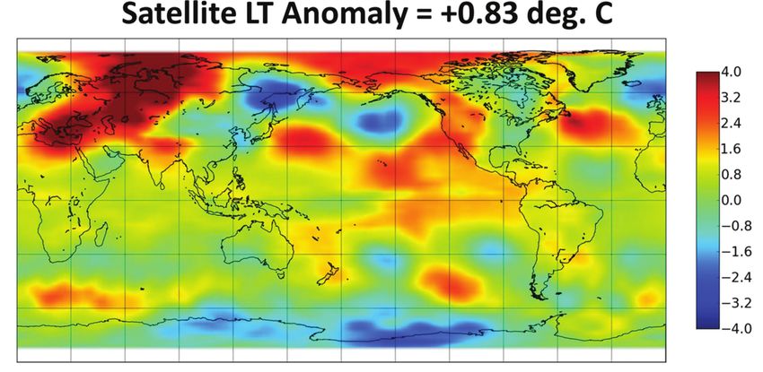
Line Charts             Scatter Plots               Bar Charts              Pie Charts              Heatmaps                 Geographical Maps

Fig. 2. Example visualization images from our corpus, each including an explicit color legend.

2     R ELATED W ORK                                                            Other projects —including ChartSense [15] and iVoLVER [21] —
                                                                             focus on semi-automated approaches, leveraging interactive annotation
Our work on color mapping extraction draws on two streams of prior
                                                                             to perform accurate chart interpretation. We similarly provide an an-
work: color design for visualization and automatic chart interpretation.
                                                                             notation interface that we use for corpus annotation; this interface can
                                                                             also be applied to correct automated extraction errors.
2.1    Color Design for Visualization
                                                                                While reading data from a chart image is one potential goal of
Colors play a central role in data visualization, as they are commonly       automatic interpretation, one might also wish to infer the program that
used to visually encode data. However, there is often a disconnect           generated the visualization. Extracting encoding specifications can be
between visualization research and visualization practice “in the wild”.     valuable for indexing and can often be performed even when occlusion
For example, Dasgupta et al. [8] report mismatches with the climate          and visual clutter render precise data extraction impossible. Poco &
research community based on a two year collaboration with domain sci-        Heer [22] present a pipeline that specializes in accurate text localization
entists. Despite the availability of decades-old design guidelines [2, 24]   and recognition within bitmap chart images, and classifies recovered
in the visualization literature, rainbow color maps are still ubiquitous.    text labels according to their role (e.g., x-axis label, y-axis label, legend
Such design choices can have serious consequences: Borkin et al. [1]         label, etc). Using these components they are able to perform accurate
found that changing the color encoding used for visualizations of arte-      extraction of spatial encodings. In this paper we follow a similar aim,
rial stress (switching from a rainbow scale to a perceptually-motivated      but focus squarely on the problem of color mapping extraction. We
palette) led to marked improvements in doctors’ diagnostic accuracy.         adopt methods from Poco & Heer [22] to recognize the text content
Unfortunately, a number of existing commercial visualization tools still     of legend labels. Siegel et al. [26] also contribute a classifier to assign
provide default color palettes of questionable quality.                      semantic roles to each text element, and use inferred legend labels to
   Meanwhile, a number of visualization projects have sought to pro-         identify legend symbols. However, they assume that text information is
vide both stock palettes and palette-generation tools to promote more        given a priori, focus only on discrete color legends, and do not recover
effective mappings between data values and colors. Cynthia Brewer’s          the color mapping. To the best of our knowledge, no prior work has
color-use guidelines [4] and popular ColorBrewer palettes are widely         proposed a technique to semi-automatically recover color mappings
used for coloring both maps and more general information visualiza-          from a static visualization image.
tions. Heer & Stone [13] demonstrate how models of color naming can             In addition to indexing and redesign applications, automatic chart
be used to assess and improve color palettes. Lin et al. [18] contribute     interpretation can enable new interactions with previously static me-
an algorithm for generating color palettes that respect “semantically res-   dia. Kong & Agrawala [16] demonstrate how to add interactivity to
onant” color-concept associations. More recently, Gramazio et al.’s Col-     static pie and bar charts. They use the ReVision system [25] to inter-
orgorical [11] tool allows designers to interactively balance concerns       pret the chart and generate graphical overlays to highlight marks and
such as discriminability, naming similarity, and aesthetic preferences.      provide guideline annotations to assist chart reading. Inspired by this
   In this work, we contribute techniques for extracting color encodings     application, we introduce a novel application that leverages extracted
from visualization images, as well as applications for automatic recolor-    color mappings to support interaction with either plotted data or color
ing and interactive overlays. To be clear, we do not contribute methods      legends to highlight and summarize values of interest. Elmqvist et
for color design. For example, our recoloring application assumes an         al. propose Color Lens [9], a technique that dynamically optimizes
appropriate target color scheme is provided as an input.                     color scales based on a set of sampling lenses. Using this technique
                                                                             we can emulate some of the features of interactive overlays; however,
2.2    Automatic Chart Interpretation & Retargeting                          Color Lens has a different goal and does not recover color mappings
                                                                             from bitmap images.
A growing body of work focuses on the “inverse problem” of data
visualization: given a visualization, can one recover the underlying
                                                                             3     DATA C OLLECTION       AND   A NNOTATION
encodings and data values? Solutions to this problem can enable auto-
mated analysis, indexing and redesign of published visualizations — in       To develop techniques for color mapping extraction, we compiled an
some cases without recourse to an original specification or dataset.         annotated corpus of visualization images using color encodings.
   Harper and Agrawala [12] introduce a system to deconstruct D3 [3]
visualizations within a web browser. By exploiting the live data binding     3.1     Image Collection
between vector graphics and backing data elements, they extract data,        We collected visualization images from both academic papers and the
marks, and mappings between them. This information can then be used          web sites of scientific institutions (e.g., NASA, universities). First we
for tasks such as redesign and style transfer.                               downloaded 16 million images from papers indexed by the Semantic
   A number of projects focus on the more difficult problem of inter-        Scholar1 search engine. These chart images come from academic
preting visualizations available only as static images. Savva et al. [25]    publications in Computer Science. In order to reduce the number of
introduce ReVision, a system to classify bitmap chart images by chart        images and promote design variability, we selected figures from the
type, automatically extract data from pie charts and bar charts, and         areas of visualization, human computer interaction, computer vision,
generate redesigns using the extracted data table. Siegel et al. [26] and    machine learning, and natural language processing. From an initial
Choudhury et al. [6, 23] present techniques to extract data from line
charts using bitmap and vectorial images, respectively.                          1 http://www.semanticscholar.org/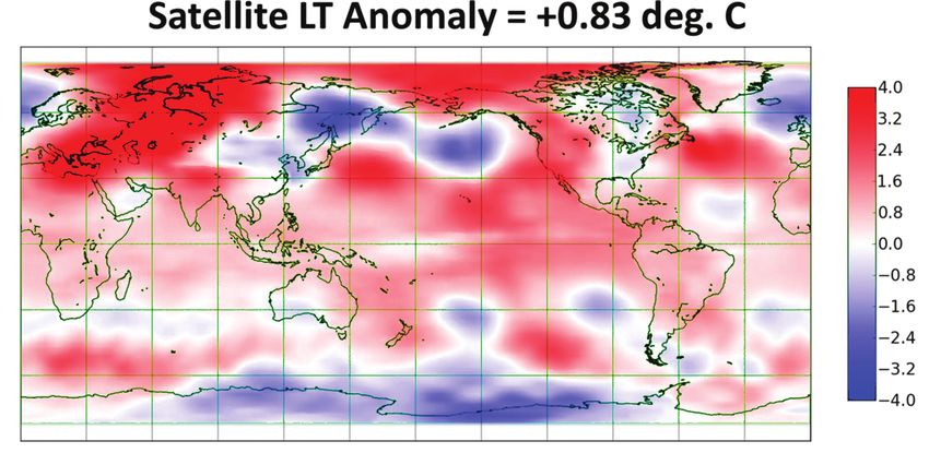
using a custom graphical interface (Figure 3). Two annotators per-
                                                                             formed these tasks, requiring roughly 20 hours to complete using our
                                                                             graphical interface.
                                                                                We define discrete color legends as consisting of a set of symbol
                                                                             elements ldisc = {e1 , e2 , ..., en }. Each symbol element is a 2-tuple
                                                                             ei = (ci ,ti ), where ci is a color and ti is the text associated with the
                                                                             color. Using our annotation interface, one can click a legend symbol
                                                                             to extract the representative color ci and its location pi . Additionally,
                                                                             to annotate the text ti associated with ci , one can draw a rectangle to
                                                                             cover the whole text element. Given the text bounding box, we attempt
                                                                             to recover the text content using the Tesseract OCR engine [27] and
                                                                             manually correct the text as needed. We store both the text content and
                                                                             bounding box information. In Figure 4(a) the yellow circles represent
                                                                             the selected pixels and the red boxes represent the text elements.
                                                                                We model continuous color legends as spatially contiguous gradients
                                                                             parameterized by the minimum and maximum extents. Thus, lcont =
                                                                             {(ci ,ti ), pmin ≤ pi ≤ pmax }, where pi is the i-th pixel position. In other
                                                                             words, a continuous color legend is represented by all the colors along
                                                                             the line between the minimum and maximum positions. To annotate
                                                                             continuous color legends within our interface, one can simply click
                                                                             the minimum and maximum positions. In Figure 4(b), these points are
                                                                             represented by the yellow circles. To recover the colors, we scan from
                                                                             pmin to pmax (for example, along the red line in Figure 4(b)). One can
                                                                             also draw rectangles next to pmin and pmax to cover the legend labels
                                                                             (red boxes in Figure 4(b)). We then apply OCR and (as needed) manual
                                                                             correction to recover the text content of the labels.

                                                                             4 C OLOR M APPING E XTRACTION M ETHOD
                                                                             Our approach comprises 5 steps: (1) color legend identification, (2)
Fig. 3. Graphical user interface for legend annotation. The bottom panel     legend classification, (3) color extraction, (4) legend text extraction,
shows chart images in our corpus. Outline colors represent the color         and (5) color mapping recovery. These steps are illustrated in Figure 5.
legend type: orange for continuous and blue for discrete.                    In step 1, we automatically detect legends that occur outside the main
                                                                             plotting area; otherwise, users can manually indicate the legend region.
                                                                             In step 2, we classify the legend as discrete, continuous, or other
                                                                             (to capture images not supported by our technique). In steps 3 and
                                                                             4, we automatically identify and process legend regions to extract
                                                                             colors and associated text, using different algorithms for the discrete
                                                                             and continuous cases. Finally, in step 5 we combine color and text
                                                                             information to recover color mappings. Across each step, we model
               (a)                                 (b)                       colors using the CIE LAB color space. All the techniques described
                                                                             in this section are trained and validated using the annotated corpus of
Fig. 4. Annotations on color legends. Note that we extract different         visualization images described in §3.
information for (a) discrete and (b) continuous legend types.
                                                                             4.1 Color Legend Identification
collection of 330,000 figures, we manually selected 1,000 chart images       Automatic legend identification is a difficult problem, as there is sig-
containing explicit color legends. We initially selected a random subset     nificant variation in both placement and arrangement (i.e., vertical,
of 200 images per category. We then removed figures without a color          horizontal, grid). While legends are sometimes placed outside the
legend and randomly selected more figures to replace them; after some        plotting area, it is also common to place them inside the plot area,
iteration, we arrived at a set of 1,000 figures. We then downloaded          particularly in academic papers where the amount of space is limited.
275 papers from three journals influential in earth sciences: Nature,        In prior work, both Siegel et. al. [26] and Poco & Heer [22] contribute
the Journal of Climate, and Geophysical Research Letters. To extract         classifiers that assign semantic roles to each text element (i.e., leg-
figures from journal PDF files, we used the pdffigures [7] utility.          end label, axis title, axis label, etc.). Legend regions could then be
We extracted 994 images and manually selected 500 chart images with          inferred based on recognized legend label and legend title elements.
color legends, using the same process for manual selection described         A shortcoming of Siegel et al.’s method is that they assume that text
previously. To further augment our collection, we crawled scientific         information is given a priori, which is not true for bitmap images. Poco
websites such as NASA and university departments (e.g., climatology          & Heer do not make this assumption and propose text localization and
& oceanography), netting 300 additional images with color legends.           recognition methods; however, these steps can still produce errors that
   In sum, our corpus contains 1,800 visualization images with color         propagate forward.
legends. We manually classified each image as representing discrete             Given the difficulty of accurate automatic legend extraction, and the
or continuous data, and selected 800 charts uniformly at random for          relative ease with which users can simply indicate a legend region with
each type. We use these 1,600 chart images for training and testing          a rectangular brush, our color extraction pipeline expects the legend
throughout this paper. Figure 2 shows examples from our corpus,              region to be given as an input. Nevertheless, in this section we present
including line charts, scatter plots, bar charts, area charts, pie charts,   a simple automatic method that does not require labeled text elements
heat maps, and geographic maps. Our only constraint for selecting            and is applicable when the legend is outside the plotting area. This
chart images was the inclusion of a color legend.                            method can be used to initialize a candidate legend region that can be
                                                                             interactively adjusted as needed.
3.2   Legend Annotation
For each visualization image, we classified the color legend as either       Method: Detection of continuous color legends is typically straightfor-
discrete or continuous, and then manually labeled the legend elements        ward, as the color gradient is commonly placed outside the plotting area.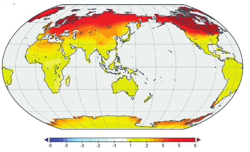
...
                                                                                                               ti  on

                                                                     us
                                                                                                            ac
                                                                                                         xtr

                                                                   uo
                                                                                                        E

                                                                    in
                                                                                                    lor

                                                                 nt
                                                                                                 Co

                                                              co
                                                                 discrete                       Tex
                                                                                                    tE   xtr
                                                                                                            ac t
                                                                                                                   ion

                                (a) Color Legend           (b) Color Legend                 (c) Color & (d) Text                  (e) Recover
                                   Identification              Classification                    Extraction                       Color Mapping

Fig. 5. Steps to infer color mappings from a chart image. (a) Localize the legend region in the chart images. (b) Use a CNN to classify the color
legend as discrete, continuous, or other. (c) Depending on the legend type, process the legend to extract colors. (d) Use OCR to recover legend text.
(e) Merge color and text information to recover the color mapping.

                                                                                                           Precision     Recall     F1-score      # Test Images
                                                                                  Discrete                     96%       96%          96%             165
                                                                                  Continuous                   97%       98%          97%             159
                                                                                  Other                        95%       94%          95%             156
                                                                                  Average / Total              96%       96%          96%             480
                                                                                               Table 1. Legend classification performance.
                (a)                                     (b)
                                                                                the other class includes random sub-images from chart images. We
Fig. 6. Automatically identified plotting areas (orange) and legends            decided to train our classifier using these sorts of images to ensure the
(green) for both (a) a continuous legend and (b) a discrete legend.             classifier results are useful for seeking user intervention if automated
                                                                                legend identification fails (i.e., it returns an incorrect legend region).
The intuition behind our method is that the plotting area will typically
be the largest connected component in the chart, and the second largest         Method: We use a Convolutional Neural Network (CNN) model for
component will be the color gradient. For example, see the heatmaps             classification. CNNs achieve state-of-the-art performance for many
and geographic maps in Figure 2. We first binarize an input image,              computer vision tasks and have been successfully used to classify the
flood fill holes, and run the connected components algorithm. We then           chart type (bar, line, scatter, etc.) of visualization images [15, 22, 26].
sort the connected components by total area and remove the largest one          Training a CNN from scratch requires a large amount of labeled training
(i.e., plotting area). Next, we search through the other components in          data, yet we have only a few thousand images in our corpus. A common
order. If the next largest component fits a rectangle, we return it as the      solution to this mismatch is to fine-tune a pre-trained network via
color gradient. Figure 6(a) shows the largest component in orange, and          backpropagation with additional images. Here, we fine-tune using the
the automatically recognized legend area in green.                              Caffe [14] implementation of AlexNet [17], pre-trained on the millions
    Discrete color legends are often placed inside the plotting area. How-      of images contained in the ImageNet dataset.
ever, if the legend has a rectangular border and is placed outside a               To train our CNN, we first extract the image regions (xl , yl , wl , hl )
well-delimited plotting area, we can apply the identical method de-             for each discrete and continuous color legend to use as examples of
scribed above for continuous legends. Figure 6(b) shows the identified          those classes. To provide examples of the other class, for each chart
plotting area and discrete legend for a line chart.                             image we additionally extract an image region (xo , yo , wo , ho ), where
    Obviously, our simple method will fail for cases that violate our           (xo , yo ) is a random coordinate and wo = r × wl , ho = r × wl , where
assumptions. Our approach could be further augmented using the                  r is a random (uniform) number between [0.9, 1.1]. We resize each
methods of Poco & Heer [22], identifying legends based on text element          extracted sub-image to a 256 × 256 pixel square, preserving aspect ratio
classification. Within user-facing applications, one can also manually          and filling empty space with a white color.
indicate a legend position by simply dragging a rectangle, as in our
annotation interface.                                                           Validation: We evaluate our classification approach using 2,400 im-
                                                                                ages across 3 categories. To maintain parity among classes, for the
Validation: Across our visualization image corpus, our simple legend            other class we sample 800 of the 1,600 randomized image regions
identification technique correctly identifies 50% (400/800) of contin-          generated above. We then randomly split the data into training (80%)
uous legends and 10% (77/800) of discrete legends. As expected, the             and test (20%) sets. Table 1 shows the resulting precision, recall and
high prevalence in our corpus of legends placed within the plotting area        F1-scores for test set classification. Across all classes, we find that our
contributes to poor performance, particularly in the discrete case. Other       classifier exhibits an average F1-score of 96%.
error cases include graphics that do not have a single dedicated plotting
area (e.g., heatmaps over multiple 3D physical models) or the presence          4.3 Color Extraction
of variable background colors.                                                  Given the color legend region and type we can proceed to extract colors,
                                                                                using different algorithms for the discrete and continuous cases.
4.2 Color Legend Classification
Once we have identified the legend region in an image, we seek to               4.3.1 Discrete Legends
classify the legend type in order to apply appropriate extraction methods.      As described in Section 3, we represent a discrete color legend as a set
We trained a classifier that takes a legend region sub-image as input           of elements ldisc = {e1 , e2 , ..., en }, where ei = (ci ,ti ). In this section,
and classifies the image into one of three color legend types: discrete,        we present a technique to extract the colors ci . As shown in Figure 7,
continuous and other. This last class is included to recognize legend           we first mask a legend image to isolate colored legend symbols and
images that are not supported by our approach. In our current version,          then use clustering to extract representative colors.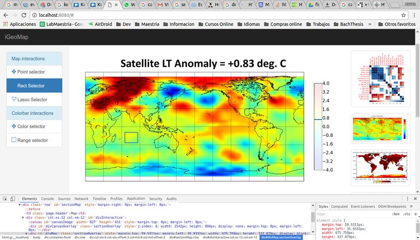
(a)                                  (b)

                (c)                                  (d)
Fig. 7. Extracting color from discrete color legends. (a) Original legend       (a)          (b)        (c)         (d)          (e)       (f )         (g)
image. (b) Mask combining background and grayscale masks. (c) Color
pixels after applying the mask. (d) Yellow circles indicate pixels with      Fig. 8. Extracting color from continuous color legends. (a) Original
representative colors found via cluster analysis.                            legend image. (b) Binarized image. (c) Flood fill to recover color gradient.
                                                                             (d) Morphological erosion to separate text from legends. (e) Connected
Method: We apply two masks to the legend image to filter extraneous          components. (f) Color gradient is the largest connected component. (g)
pixels: a background mask and a grayscale mask. We infer the back-           Yellow circles indicate positions of minimum and maximum values.
ground color cbg by computing a color histogram for all pixels in the
legend image and selecting the most frequent color. In most cases the
background color is white. As pixel colors may be noisy, we consider         our visualization corpus. We use precision, recall and F1-score metrics
a pixel part of the background if its color ci is in the range cbg ± Tbg ,   typically used for comparing inferred bounding boxes in the context of
where we set Tbg = 5 (or approximately two JNDs [20]).                       text localization [19]. However, in our case, we compare two sets of
   We consider a color ci to be grayscale if both its a and b LAB            colors (estimated and ground truth) instead of bounding boxes.
components lie in the range 0 ± Tgray (again, setting Tgray = 5). The           For a color c we find the best match in a set of colors S such that:
grayscale mask is useful for removing grid lines and text; however, it
can also remove pixels that belong to a symbol encoded with a gray                                   m(c, S) = min
                                                                                                                0
                                                                                                                   distcolor (c, c0 )                      (1)
color. We describe how we recover those pixels later in this section.                                            c ∈S
   Applying these masks leaves the pixels for the legend col-
                                                                                where distcolor (ci , c j ) is the CIEDE2000 color difference.
ors. Figure 7(b) shows the combined mask, and Figure 7(c)
                                                                                We apply this best matching to align the ground truth legend colors
shows the resulting colored pixels. Note that the colors for each
                                                                             T and estimated colors E. We define δ (ci , c j ) = dist(ci , c j ) < 5. Note
symbol might not be homogeneous, especially
                                                                             that δ is 1 if two colors are within 5 CIE LAB units, 0 otherwise. We
along the symbol edges. As the color values
                                                                             noticed that comparing colors (ci , c j ) in the representative pixels (pi , p j )
are noisy and also potentially discontinuous
                                                                             can be very sensitive, specially when legend symbol is a segment line.
(see inline figure), we can not use simple color binning or connected
                                                                             This problem arises specially in annotated data. To address this issue,
components analysis. We need a more robust approach for grouping
                                                                             we use patch regions centered at representative pixels (pi ) and width
pixels with similar color.
                                                                             3. Thus, dist(ci , c j ) returns the minimum color difference between
   We apply a clustering algorithm to identify the legend colors.            patches centered at pi and p j .
We represent each colored pixel using a five-dimensional feature                We define precision, recall and F1-score as follows:
vector consisting of the three LAB color chan-
nel values plus the x and y image pixel co-                                             ∑ δ (e, m(e, T ))          ∑ δ (t, m(t, E))
ordinates: (L, a, b, x, y). In most cases, color                                       e∈E                         t∈T                            p·r
                                                                                 p=                         , r=                       , F1 = 2            (2)
information is enough to groups the pixels. However, some legends                              |E|                        |T |                    p+r
have colors with the same hue but varying luminance (see inline figure).
In such cases our clustering algorithm could fail if the colors are near        Our technique has a precision of 92%, recall of 89%, and F1-score
each other in the CIELAB space. Pixel coordinates help to separate           of 90% in our 800 discrete color legends.
these cases.
   We then use the DBSCAN [10] clustering algorithm. DBSCAN does             4.3.2 Continuous Legends
not require that the number of clusters be chosen a priori, and accepts      In this section, we describe how to extract colors for a continuous
parameters that are well defined for our setting. The ε parameter            legend. To characterize a continuous color legend, we must identify the
sets the maximum distance for two points to be considered in the             color gradient end points pmin and pmax . We record the pixel locations
same neighborhood; we use ε = 5. The minPoints parameter sets the            for each end point and extract colors by scanning the line between the
minimum number of points in a cluster. We assume that a color legend         two. Figure 8 illustrates each step in this technique.
has at most 20 symbols and so minPoints = |color pixels|/20.
   For each resulting cluster gi , we then select the most common color      Method: Akin to the discrete case, we first infer the back-
to be the representative legend color ci . Figure 7(d) shows the locations   ground color and remove background pixels. Next, we bi-
of pixels with representative colors (yellow circles).                       narize the legend image using a global threshold approach.
   As mentioned earlier, our grayscale mask may erroneously remove           Note that the bottom part of the color gradient in Figure 8(b)
pixels that belong to gray-colored legend symbols. To recover such pix-      is incomplete. To recover such regions, we use a flood fill
els, we run the connected components algorithm within the grayscale          algorithm. Figure 8(c) shows the completed region.
mask, and retrieve components with an area (i.e., number of pixels)              We noted that in some charts the text elements are very
similar to the area of the discovered clusters gi .                          close to the colorbar (see inline figure). To separate them,
                                                                             we apply a morphological erosion operation (Figure 8(d)). Then we
Validation: We evaluate our discrete color extraction method against         run the connected components algorithm (Figure 8(e)). Our intuition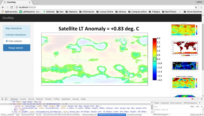
(a)

                                                                                        (a)                                        (b)
                                   (b)                                         Fig. 10. Recovering color-value mappings for discrete legends. In (a), we
                                                                               associate text with the nearest legend symbol. For multi-column legends
                                                                               (b), we first identify if the text is on the right or left of the legend symbols.
Fig. 9. Analysis of quantized legends for continuous data. (a) Some
legends discretize a quantitative domain. (b) Breaks between colors
correspond to peaks in the absolute derivative of pixel color.

is that the color gradient should be the largest connected component
and all the text characters should be smaller. Thus, we select the largest
component (Figure 8(f)) and fit a rectangle that covers these pixels. We
note if the rectangle has a vertical or horizontal orientation based on its
aspect ratio. If vertical, we determine pmin and pmax by selecting two
aligned points, one at the top and one at the bottom side of the rectangle,
each horizontally centered. Scanning a line that join these two points,
we recover the colors belonging to this legend (See Figure 8(g)). An           Fig. 11. Recovering color-value mappings for continuous color legends.
                                                                               Values in bounding boxes ble f t and bright are mapped to positions ple f t
analogous approach applies for the horizontal case.
                                                                               and pright , respectively. We then extrapolate values for pmin and pmax .

Validation: We evaluate continuous legend color extraction on the 800
continuous examples in our corpus. For each image, we estimate pmin            we apply optical character recognition to each candidate word using the
and pmax using the method above and compare these two points with              open source Tesseract [27] engine. Finally, in stage 3, words are merged
the ground truth data p0min and p0max . For a vertical rectangle, we deem      into phrases based on their orientation and geometric relationships.
two points similar if |py − p0y | < 3 (i.e., the y-coordinates are at most 3      Before submitting legend images to the text localization pipeline,
pixels away). If both pmin and pmax lie near the ground truth values, we       we remove all pixels that belong to either discrete legend symbols or
consider the color gradient to have been successfully identified. The          continuous color gradients. This preprocessing step cleans the input
horizontal case is treated similarly.                                          images in order to improve text localization performance.
   Our method achieves accurate extraction for 83% (662/800) of the
continuous legends in our corpus. Recurring error cases involve con-
fusion between the color gradient and background colors (i.e., when a          Validation: To evaluate the text extraction technique, we use the defi-
color gradient is placed within the plotting area) and confusion due to        nition of best matching depicted in Section 4.3.1 (Equation 1), but in
text labels placed so close to the gradient that they become part of the       our case, we compare two sets of boxes (estimated and ground truth)
same connected component. Perhaps ironically, this first error case is         instead of colors. For a box b, we find the best match in a set of boxes
most prevalent in the visualization literature, as other disciplines tend      S such that:
to place the color gradient outside the plotting area.                                                  m(b, S) = max
                                                                                                                   0
                                                                                                                      distbox (b, b0 )                      (3)
                                                                                                                   b ∈B

Quantized Continuous Domains: It is common to use discretized                                                    2 area(b ∩b )
                                                                                                                         i  j
version of continuous legends (Figure 9(a)). Our color legend classifier          Where, distbox (bi , b j ) = area(b )+area(b    . Note that distbox is 1 for
                                                                                                                     i         j)
classifies these legends as continuous, and we process them using our          equal boxes and 0 for boxes without intersection. We then apply
continuous color extraction methods (i.e., determining pmin and pmax ).        this matching to our bounding boxes T (ground truth boxes) and E
However, we can then perform a post-processing step to properly handle         (estimated boxes) in a legend image. We define precision, recall and
this legend type.                                                              F1-score as follows:
   Consider the horizontal color gradient in Figure 9(a). First we
compute the horizontal derivative to identify strong changes along the                            ∑ m(e, T )          ∑ m(t, E)
x-axis. We apply a Sobel filter with a kernel of size 3. Figure 9(b)                             e∈E                  t∈T                     p·r
                                                                                           p=                  , r=                , F1 = 2                 (4)
shows the absolute values of this derivative (computed as the sum of r,                                |E|                  |T |              p+r
g, and b color channel derivatives). We next convolve the data with a
wavelet of size 10 (this value is the expected range that should cover            Using only the discrete color legends we obtain a precision of 82%,
the peaks of interesest) and extract the peaks. Given k identified peaks,      recall 91% and F1-score 86%. If we do not remove the colored pixels
we extract a set of k + 1 colors by picking the colors at the midpoints        beforehand the F1-score is 83%; the OCR results are meaningfully
between peaks, or between the legend boundary and nearest peak.                improved by this filter. In addition, these performance results are very
                                                                               sensitive to the bounding boxes. For example, if we shrink or expand
4.4 Legend Text Extraction                                                     the ground truth boxes by 2 pixels, the F1-scores reduce to values
The previous sections describe how we extract colors for discrete and          between 82% and 85%. The main errors arise when legend symbols
continuous legends. We now present a method for recovering text                contain multiple colors, in which case our preprocessing can fail to
elements from a legend image (Figure 5(d)).                                    remove those pixels.
                                                                                  Using the continuous color legends we obtain a precision of 78%,
Method: We first apply the text localization method of Poco &                  recall 79% and F1-score 78%. The main issues arise with tick marks. A
Heer [22]. This approach consists of three stages: (1) word detec-             tick may be confused with the ‘-’ character, extending the text bounding
tion, (2) optical character recognition, and (3) word merging. In stage        box. In some cases ticks connect the text with the color gradient,
1, a CNN trained to classify text vs. non-text pixels is used to mask          causing the text localization step to throw out text along with the color
non-text pixels. Then, standard region-based text localization methods         gradient. Across both legend types, we obtain an overall precision of
are applied to output bounding boxes for individual words. In stage 2,         80%, recall 85% and F1-score 82%.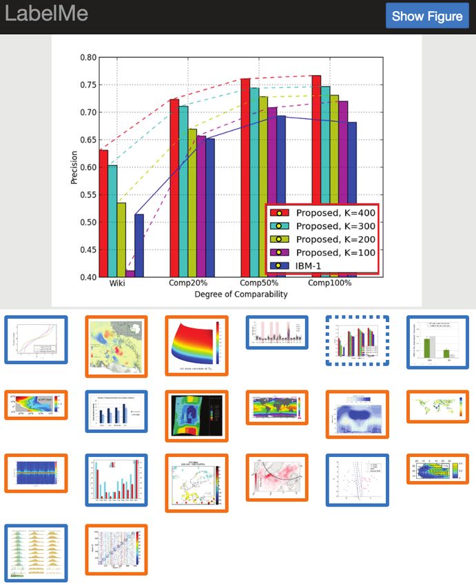
Discrete                                                                   Continuous
             (a)                           (b)                                     (c)                                  (d)
Original

             (e)                           (f )                                    (g)                                  (h)
Recolored

Fig. 12. Automatic Recoloring: Given a chart image and target color scheme, we generate a recolored image with an alternative color encoding.

4.5          Recovering Color Mapping                                          error propagation (see discussion by Poco & Heer [22]). Instead, we
Given the color information and the text extracted in the last two             assume the legend regions are provided as input, as it is relatively easy
sections, we can recover the full color mapping. To do so, we need to          for a user to drag a rectangle over them.
associate the text values with the color information (Figure 5(e)).               The validations presented in §4 assume that output from a previous
                                                                               step is perfect. However, without user intervention, an error gener-
                                                                               ated in an earlier step can propagate through the pipeline, reducing the
Discrete color legends: Here, we connect each text bounding box with           final accuracy. As mentioned above, we present our results without
a legend symbol — represented by a pixel inside the legend symbol.             interdependence of the pipeline steps. Though users can manually fix
For each text bounding box, we calculate the closest legend symbol and         interpretation errors using our annotation interface, for some applica-
associate this text with the color. This strategy also works for legends       tions (e.g., analysis of visualizations practices “in the wild”) a fully
with multi-line text (Figure 10(a)). However, for horizontally-aligned         automatic method is required.
elements or multiple columns, this strategy can fail. In Figure 10(b),            For an end-to-end analysis, we assume legend regions are given as
the legend text “Roc-SVM” might be considered closest to the brown             input to our pipeline. Our color and text extraction components then
legend symbol for “CR-EM”. To address this issue, we must determine            depend on the output of legend type classification. However, there is no
if text lies to the left or right of the legend symbols. We first sort by      interdependence between color and text extraction: both steps can be
x-coordinate of the representative pixels for each legend symbol. Next         performed in parallel as shown in Figure 5. For discrete color legends,
we check if the left-most and right-most pixel are closer to the left or       we achieve local F1-scores of 96% in the legend classification step,
right side of the legend bounding box, respectively. If the left-most          90% in the color extraction step, and 87% in the legend text extraction
pixel is closer, then text lies to the right (See Figure 10(b)), otherwise     step. If we propagate errors, we have final F1-scores of 82% for color
text lies to the left.                                                         extraction and 80% for the legend text extraction. For continuous color
                                                                               legends, we have local F1-scores of 96% in the legend classification
 Continuous color legends: We first identify if the legend gradient is         step, 82% in the color extraction step, and 80% in the legend text
vertically or horizontally oriented. We do so by checking the alignment        extraction step. If we propagate errors, we have final F1-scores of 79%
 of the pmin and pmax coordinates. For the horizontal case, we sort the        for color extraction and 77% for the legend text extraction.
 text bounding boxes by the x-coordinate of their centers. We denote the
 center of the left-most and right-most text bounding boxes with ple f t       6     A PPLICATIONS    OF   C OLOR M APPING E XTRACTION
 and pright respectively (see Figure 11). We map the value represented
 by the text in both bounding boxes to ple f t and pright , respectively.      Our extraction methods can be used to support a variety of visualization
 Finally, we extrapolate the values out to pmin and pmax . An analogous        applications. For example, our work can be used to extend existing visu-
 approach applies for the vertical case.                                       alization reverse-engineering tools [15,22,25,26] with support for color
    In order to extract the values represented by the text, we first attempt   encodings, improving tasks such as indexing for visualization search
 to parse the label text as number, including scientific notation (e.g.,       engines [5]. Here, we contribute two novel user-facing applications:
‘-10’, ‘15’, ‘4.5’, ‘3e-4’). Next, we verify if there is a modifier, such as   automatic recoloring and interactive overlays.
 characters indicating units. We check if the text is using International
 System units (e.g., ‘1M, ‘1k, ‘10M) and parse these as numbers (e.g.,         6.1       Automatic Recoloring
‘1k’ is converted to 1,000). We leave text parsing of other cases, such        Our first application performs automatic recoloring: given bitmap im-
 as physical units of measurement, as future work.                             ages as input, we produce new images that use perceptually-motivated
                                                                               color encodings. This application works for both discrete and contin-
5           E ND - TO -E ND P ERFORMANCE                                       uous color legends. Figure 12 shows examples for four chart images:
At first blush our pipeline might look complex, given the multiple             the first row contains original visualizations and the second row shows
processing stages. An alternative approach might be to analyze a color         output images with new color encodings.
histogram for each image and skip the color legend identification step.           Discrete color legends. Given representative colors C = {c1 , ..., cn }
However, we found that the unbalanced number of pixels for each                inferred by our extraction methods and a target color scheme T =
color makes subsequent color extraction less accurate. Moreover, to            {t1 , ...,tn }, we create a transfer function ti = fdisc (ci ) that simply maps
automatically infer a color mapping one must identify the legend region.       from one indexed color to another. For each pixel pi in the image, we
This step could increase the complexity of our pipeline and suffer from        find the nearest color in C such that distcolor (ci , cs ) < 2.5 and then set
Discrete                                                          Continuous

                      (a)                         (b)                             (c)                                  (d)
Original

                      (e)                         (f)                             (g)                                  (h)
From Legend to Plot

                      (i)                         (j)                             (k)                                  (l)
From Plot to Legend

                                                                                                      (m)
Fig. 13. Interactive Overlays. The first row contains input chart images. The second row shows interactive highlights of the data in response to
selecting legend values. The third row illustrates highlights in response to selecting marks in the plotting area. Sub-figure (m) shows a value
histogram for the selected pixels, generated by inverting the extracted color mapping.

pi to the color fdisc (ci ). The distance constraint helps avoid recoloring     our extraction techniques. If a user notes any extraction errors, they
pixels that do not belong to the color legend (e.g., grid lines or text).       can use our annotation interface (§3.2) to correct them manually. The
   The bar chart in Figure 12(a) uses a sequential color encoding where         application then generates an interactive visualization that supports
a categorical encoding might be more appropriate. In Figure 12(e),              two-way interactions between the legend and plotting area. Users can
our tool replaces the original scheme with a ColorBrewer palette. The           brush in either region to see corresponding information highlighted in
line chart in Figure 12(b) uses a discrete rainbow color map. Some              the other component. Figure 13 shows examples of such interactions
legend items (e.g., “RNN1” and “RNN4”) are difficult to discriminate.           across four different chart types.
In Figure 12(f) we retarget the color encoding to a more perceptually              From legend to plot area. We provide two types of interactions:
effective scheme.                                                               point and range selection. These interactions are designed to highlight
   Continuous color legends. For continuous legends, we begin with              selected data values, as illustrated in the second row of Figure 13.
the extracted colors spanning the minimum and maximum points in                    Point selection is supported for both discrete and continuous color
the color gradient ({ci | pmin < pi < pmax }), and a target continuous          legends. For discrete legends, users can click either a legend symbol
color palette T parameterized on the interval [0, 1]. We define a transfer      or the text associated with the symbol. We then identify the associated
function ti = fcont (ci ), such that ci and ti occur at the same relative       representative color csel . Next, we overlay the plotting area with a
index in their respective color ramps. For each pixel pi in the image,          translucent white layer, using full transparency for pixels pi that satisfy
we search for the nearest color in C such that distcolor (ci , cs ) < 2.5 and   distcolor (csel , ci ) < 2.5. If the legend is inside the plot area (as in
recolor the pixel with fcont (ci ).                                             Figure 13(e)), we make that region transparent as well. For continuous
   The map in Figure 12(c) uses a multi-hue color gradient across               color legends, a user can click anywhere within the color gradient to
a domain spanning both negative and positive values. In response,               select the color csel . Then, we similarly add a translucent overlay, but
we recolor the image using a diverging color scheme as shown in Fig-            with full transparency for pixels pi that satisfy ci = csel .
ure 12(g). Figure 12(d) uses a rainbow color scheme; in Figure 12(h) we            Range selection is often more appropriate for continuous color leg-
replace the rainbow with a perceptually-informed sequential scheme.             ends. When a user draws a rectangle (R) within the color gradient, we
   For these recoloring tasks, we need only extract the color information       select the set of colors Csel = {ci | pi ∈ R}. As with point selection,
provided in the legend. The actual legend text is not necessary, making         we then add a translucent overlay with full transparency for pixels that
our tool robust to issues such as OCR error. However, as our next               satisfy ci = cs , ∀cs ∈ Csel .
application demonstrates, recovering the legend values can enable more             From plot area to legend. For interactions with the plot area, we
sophisticated interactions.                                                     similarly support both point and range selections. These interactions
                                                                                are depicted in the third row of Figure 13.
6.2                   Interactive Overlays                                         Point selections can be performed visualizations with either discrete
Our second application adds interactive overlays [16] to static images to       or continuous color legends. For discrete legends, users can click a
support data querying and highlighting. Our web application generates           data-encoding mark in the plot area. We then select the color csel
an interactive visualization from a static image input.                         at the click position psel , and use it to identify the legend element
    First, the system must locate the color legend. If automated iden-          esel with representative color nearest to csel . Next, we overlay the
tification (§4.1) fails, a user can simply draw a rectangle to isolate          legend region with a translucent white layer. We use the information
the legend. Next we recover legend color and text information using             in esel (i.e., text and color) to make the layer transparent over pixels
that lie inside the text bounding box or satisfy csel = color(esel ). We         8 C ONCLUSION
also add a layer over the plot area, with full transparency for pixels           In this paper we presented methods for recovering color mappings from
that satisfy distcolor (csel , ci ) < 2.5. In this second layer highlights all   static visualization images. To evaluate our approach we compiled an
marks associated with the same esel (for instance, the multiple bars             annotated corpus of images and color legend information for 1,600
highlighted in Figure 13(i)). For continuous legends, when a user clicks         visualizations from academic documents, and demonstrated accurate
in the plot area we select the color csel and search for the nearest color       extraction of both discrete and continuous color encodings. While
in the legend. We proceed as before to highlight pixels in the plot area.        we focused on the general case of bitmap images, components of our
However in the legend region, we highlight only the nearest color in             system are directly applicable to structured image formats such as
the color gradient.                                                              vector PDF or SVG documents, where objects and text content might
   Our tool also supports range selections for continuous encodings. A           be trivially extracted.
user can draw a rectangle (R) in the plot area, for which we retrieve                We also presented applications of our method for automatic re-
all contained colors Csel = {ci | pi ∈ R}. Then, for all colors in Csel ,        coloring and generating interactive visualizations from static images.
we find the nearest colors in the legend gradient and highlight them             Conveniently, many of the features of these applications do not require
(Figure 13(k)). In this case, we do not add an overlay to the plot area.         the full mapping from color to data value, for example supporting re-
   The interactions described above require only color information from          coloring and highlighting based on extracted colors alone. However, as
the legend. However, we can use the full mapping (i.e., inferred data            demonstrated by interactive overlay application, access to the full color
values) to enable additional features. Our tool calculates and displays          mapping can provide even richer interactive capabilities.
descriptive statistics for the data values indicated by the selected pixels.         To the best of our knowledge, this research contributes the first
For example, Figure 13(m) uses the data values associated with the               approach to recover full color mappings from visualization images.
colors in Csel to create a histogram for the selected region.                    Going forward, we hope to improve our methods and explore additional
                                                                                 applications enabled by our approach.
7   L IMITATIONS                                                                     An immediate future work item is to further improve the performance
Our color legend classifier includes the category other, which we train          of each stage in our pipeline, for example by addressing the limitations
using random sub-images sampled from our corpus. An improvement                  enumerated above. Looking further out, we might also extend our
would be to collect real legend images for other encoding channels               techniques to recover mappings for other non-spatial channels, such
(e.g., size, shape) and train our classifier to discriminate those.              as size, shape, and texture encodings. We might also extend our work
    Given the variability of color legend styles, we constrained the color       to support bi/trivariate color maps. Combining legend analysis with
legend types supported. For example, we do not support grayscale                 reverse-engineering pipelines for spatial encodings [15, 22, 25, 26]
legends. Our color extractor for discrete color legends uses a grayscale         might enable rich indexing of visualizations, in turn supporting new
mask to remove text and grid elements from the legend. As a result,              visualization search and retrieval applications.
all legend symbols in grayscale are also removed. However, if not all                Another area for future work is to perform a more thorough com-
the legend symbols are grayscale, we can recover them as explained               parison with previous approaches. The closest work is Siegel et al.’s
in § 4.3.1. We also do not support bi/trivariate color maps, which are           approach [26] to extract legend symbols from discrete color legends.
uncommon in the figures we collected. In the case of legend symbols              An appropriate comparison would be to run our pipeline on Siegel et
with repeated colors (e.g., “red” symbol with a solid line and “red”             al.’s annotated image dataset (1,000 annotated charts). For that, we will
symbol with a dashed line), our color extractor might fail because we            need to parse the figure metadata and infer the legend regions using the
are using LAB coordinates in the clustering, and all the red pixels will         bounding boxes of the legend text and legend symbols. However, com-
be near each other in the CIELAB space.                                          paring text elements would be unfair because Siegel et al. assume that
    In the legend text recognition step, we use the techniques of Poco           the text information is given as input. Also, in Siegel et al.’s dataset the
& Heer [22]. However, OCR errors remain an issue in some cases.                  legend symbols are annotated using bounding boxes; to compare with
Recurring challenges for text localization include the resolution of             our color extraction method, we will need to process each bounding
the legend labels, spacing between labels and color elements, and                box region and extract the colors used.
mathematical notation. Moreover, in this work we are not using the                   We might also use our color extraction techniques to perform a large
“units” information included in some continuous color legends. For               scale analysis of the use of colors “in the wild”. We can analyze a large
applications such as indexing figures (e.g. for a scientific database),          collection of visualization images from academic documents across
accurately identifying units may be important.                                   different communities, identify common color schemes, and assess how
    We currently do not support accurate data value interpolation for            they may have evolved or disseminated over time.
non-linear color gradients. To do so, our method must also (a) extract               To help enable such future applications, both our annotated visualiza-
intermediate value labels (not only minimum and maximum), (b) cor-               tion image corpus and the source code for our color mapping extraction
rectly associate the labels with positions in the color gradient, and (c)        methods are freely available at https://github.com/uwdata/rev.
infer the the type of scale function (e.g., log, square root) based on
the label values and spacing. Step (c) is relatively straightforward and         ACKNOWLEDGMENTS
supported in prior work [22]. However, step (a) depends heavily on               This work was supported by a Paul G. Allen Family Foundation Dis-
OCR accuracy.                                                                    tinguished Investigator Award and the Moore Foundation Data-Driven
    For our recoloring application, errors arise when                            Discovery Investigator program. The second author gratefully acknowl-
the legend includes colors that also occur in other                              edges CONCYTEC for a scholarship in support of graduate studies.
chart components (e.g., black for text and grid lines,
white for background). In Figure 12(g), the chart
title was affected by our transfer function because the
initial color gradient contains black as well.
    In addition, we found that some bar charts contain
elements with variable colors (e.g., gradient fills).
This can lead to the same color occurring across
marks associated with different legend elements. For
instance, in the inline figure, the colors inside the two yellow rectangles
are the same, even though the two bars correspond to different legend
entries. As a result, our interactive overlay application does not high-
light the bars correctly. A more sophisticated color matching model is
needed to handle cases such as these shading gradients.
R EFERENCES                                                                               S. Guadarrama, and T. Darrell. Caffe: Convolutional architecture for
 [1] M. Borkin, K. Gajos, A. Peters, D. Mitsouras, S. Melchionna, F. Rybicki,             fast feature embedding. arXiv preprint arXiv:1408.5093, 2014.
     C. Feldman, and H. Pfister. Evaluation of artery visualizations for heart     [15]   D. Jung, W. Kim, H. Song, J.-I. Hwang, B. Lee, B. Kim, and J. Seo.
     disease diagnosis. IEEE Transactions on Visualization and Computer                   ChartSense: Interactive data extraction from chart images. In ACM Human
     Graphics, 17(12):2479–2488, 2011.                                                    Factors in Computing Systems (CHI), 2017.
 [2] D. Borland and R. M. Taylor. Rainbow color map (still) considered             [16]   N. Kong and M. Agrawala. Graphical overlays: Using layered elements
     harmful. Computer Graphics and Applications, 27(2):14–17, 2007.                      to aid chart reading. IEEE Transactions on Visualization and Computer
 [3] M. Bostock, V. Ogievetsky, and J. Heer. D3: Data-Driven Documents.                   Graphics, 18(12):2631–2638, 2012.
     IEEE Trans. Visualization & Comp. Graphics (Proc. InfoVis), 2011.             [17]   A. Krizhevsky, I. Sutskever, and G. E. Hinton. Imagenet classification
 [4] C. A. Brewer. Color use guidelines for data representation. In Proceedings           with deep convolutional neural networks. In F. Pereira, C. J. C. Burges,
     of the Section on Statistical Graphics, American Statistical Association,            L. Bottou, and K. Q. Weinberger, eds., Advances in Neural Information
     pp. 55–60, 1999.                                                                     Processing Systems 25, pp. 1097–1105. Curran Associates, Inc., 2012.
 [5] Z. Chen, M. Cafarella, and E. Adar. DiagramFlyer: A search engine for         [18]   S. Lin, J. Fortuna, C. Kulkarni, M. Stone, and J. Heer. Selecting
     data-driven diagrams. In Proceedings of the 24th International Conference            semantically-resonant colors for data visualization. Computer Graph-
     on World Wide Web, WWW ’15 Companion, pp. 183–186. ACM, New                          ics Forum (Proc. EuroVis), 2013.
     York, NY, USA, 2015.                                                          [19]   S. M. Lucas. ICDAR 2005 text locating competition results. In Eighth
 [6] S. R. Choudhury, S. Wang, and C. L. Giles. Scalable algorithms for                   International Conference on Document Analysis and Recognition (IC-
     scholarly figure mining and semantics. In Proceedings of the International           DAR’05), pp. 80–84 Vol. 1, Aug 2005.
     Workshop on Semantic Big Data, SBD ’16, pp. 1:1–1:6. ACM, New York,           [20]   M. Mahy, L. Van Eycken, and A. Oosterlinck. Evaluation of uniform color
     NY, USA, 2016.                                                                       spaces developed after the adoption of cielab and cieluv. Color Res. Appl.,
 [7] C. Clark and S. Divvala. Pdffigures 2.0: Mining figures from research                19(2):105–121, 1994.
     papers. In Proceedings of the 16th ACM/IEEE-CS on Joint Conference on         [21]   G. G. Méndez, M. A. Nacenta, and S. Vandenheste. iVoLVER: Interactive
     Digital Libraries, JCDL ’16, pp. 143–152. ACM, New York, NY, USA,                    visual language for visualization extraction and reconstruction. In Pro-
     2016.                                                                                ceedings of the 2016 CHI Conference on Human Factors in Computing
 [8] A. Dasgupta, J. Poco, Y. Wei, R. Cook, E. Bertini, and C. Silva. Bridging            Systems, CHI ’16, pp. 4073–4085. ACM, New York, NY, USA, 2016.
                                                                                   [22]   J. Poco and J. Heer. Reverse-engineering visualizations: Recovering visual
     theory with practice: An exploratory study of visualization use and design
                                                                                          encodings from chart images. Computer Graphics Forum (Proc. EuroVis),
     for climate model comparison. IEEE Transactions on Visualization and
                                                                                          36(3):353–363, 2017.
     Computer Graphics, 21(9):996–1014, Sept 2015.
                                                                                   [23]   S. Ray Choudhury, S. Wang, and C. L. Giles. Curve separation for line
 [9] N. Elmqvist, P. Dragicevic, and J.-D. Fekete. Color lens: Adaptive color
                                                                                          graphs in scholarly documents. In Proceedings of the 16th ACM/IEEE-CS
     scale optimization for visual exploration. IEEE Trans. Vis. Comput. Graph.,
                                                                                          on Joint Conference on Digital Libraries, JCDL ’16, pp. 277–278. ACM,
     17(6):795–807, 2011.
                                                                                          New York, NY, USA, 2016.
[10] M. Ester, H.-P. Kriegel, J. Sander, and X. Xu. A density-based algorithm
                                                                                   [24]   B. E. Rogowitz, L. A. Treinish, and S. Bryson. How not to lie with
     for discovering clusters in large spatial databases with noise. In Proc. of
                                                                                          visualization. Computers in Physics, 10(3):268–273, 1996.
     2nd International Conference on Knowledge Discovery and, pp. 226–231,
                                                                                   [25]   M. Savva, N. Kong, A. Chhajta, L. Fei-Fei, M. Agrawala, and J. Heer.
     1996.
                                                                                          ReVision: Automated classification, analysis and redesign of chart images.
[11] C. C. Gramazio, D. H. Laidlaw, and K. B. Schloss. Colorgorical: Creating
                                                                                          In Proceedings of the 24th Annual ACM Symposium on User Interface
     discriminable and preferable color palettes for information visualization.
                                                                                          Software and Technology, UIST ’11, pp. 393–402. ACM, New York, NY,
     IEEE Transactions on Visualization and Computer Graphics, 23(1):521–
                                                                                          USA, 2011.
     530, 2017.
                                                                                   [26]   N. Siegel, S. Divvala, and A. Farhadi. FigureSeer: Parsing result-figures in
[12] J. Harper and M. Agrawala. Deconstructing and restyling d3 visualizations.
                                                                                          research papers. In Proceedings of the European Conference on Computer
     In Proceedings of the 27th Annual ACM Symposium on User Interface
                                                                                          Vision, ECCV ’16, 2016.
     Software and Technology, UIST ’14, pp. 253–262. ACM, New York, NY,
                                                                                   [27]   R. Smith. An overview of the tesseract ocr engine. In Proceedings of
     USA, 2014.
                                                                                          the Ninth International Conference on Document Analysis and Recog-
[13] J. Heer and M. Stone. Color naming models for color selection, image
                                                                                          nition - Volume 02, ICDAR ’07, pp. 629–633. IEEE Computer Society,
     editing and palette design. In ACM Human Factors in Computing Systems
                                                                                          Washington, DC, USA, 2007.
     (CHI), 2012.
[14] Y. Jia, E. Shelhamer, J. Donahue, S. Karayev, J. Long, R. Girshick,
You can also read