Weed Classification Using Explainable Multi-Resolution Slot Attention
←
→
Page content transcription
If your browser does not render page correctly, please read the page content below
sensors
Article
Weed Classification Using Explainable Multi-Resolution
Slot Attention
Sadaf Farkhani * , Søren Kelstrup Skovsen                       , Mads Dyrmann          , Rasmus Nyholm Jørgensen
and Henrik Karstoft

                                          Department of Electrical and Computer Engineering, Aarhus University, 8200 Aarhus, Denmark;
                                          ssk@ece.au.dk (S.K.S.); madsdyrmann@ece.au.dk (M.D.); rnj@agrointelli.com (R.N.J.); hka@ece.au.dk (H.K.)
                                          * Correspondence: farkhanis@ece.au.dk

                                          Abstract: In agriculture, explainable deep neural networks (DNNs) can be used to pinpoint the
                                          discriminative part of weeds for an imagery classification task, albeit at a low resolution, to control
                                          the weed population. This paper proposes the use of a multi-layer attention procedure based on a
                                          transformer combined with a fusion rule to present an interpretation of the DNN decision through a
                                          high-resolution attention map. The fusion rule is a weighted average method that is used to combine
                                          attention maps from different layers based on saliency. Attention maps with an explanation for
                                          why a weed is or is not classified as a certain class help agronomists to shape the high-resolution
                                          weed identification keys (WIK) that the model perceives. The model is trained and evaluated on two
                                          agricultural datasets that contain plants grown under different conditions: the Plant Seedlings Dataset
                                          (PSD) and the Open Plant Phenotyping Dataset (OPPD). The model represents attention maps with
                                          highlighted requirements and information about misclassification to enable cross-dataset evaluations.

                                   State-of-the-art comparisons represent classification developments after applying attention maps.
Citation: Farkhani, S.; Skovsen, S.K.;
                                          Average accuracies of 95.42% and 96% are gained for the negative and positive explanations of the
Dyrmann, M.; Jørgensen, R.N.;             PSD test sets, respectively. In OPPD evaluations, accuracies of 97.78% and 97.83% are obtained for
Karstoft, H. Weed Classification          negative and positive explanations, respectively. The visual comparison between attention maps also
Using Explainable Multi-Resolution        shows high-resolution information.
Slot Attention. Sensors 2021, 21, 6705.
https://doi.org/10.3390/s21206705         Keywords: transformer; slot attention; explainable neural network; fusion rule; weed classification;
                                          weed identification key; precision agriculture
Academic Editors: Asim Biswas,
Dionysis Bochtis and Aristotelis C.
Tagarakis

                                          1. Introduction
Received: 30 June 2021
Accepted: 1 October 2021
                                               Weeds compete with crops to capture sunlight and take up nutrients and water; this
Published: 9 October 2021
                                          competition leads to significant yield losses around the world every year [1]. Furthermore,
                                          there are considerable indirect negative externalities that should be taken into consideration
Publisher’s Note: MDPI stays neutral
                                          when combating weeds [2]. Currently, the use of conventional weed control methods
with regard to jurisdictional claims in
                                          usually results in soil erosion, global warming, and human health problems [3–6]. Weeds
published maps and institutional affil-   are usually not distributed evenly across farmlands. Therefore, weed management could
iations.                                  be greatly improved by collecting information about the location, type, and amount of
                                          weeds in an area [7].
                                               In general, there are three primary weed management strategies: biological, chemical,
                                          and physical [8]. Biological weed management refers to weed control through the use
Copyright: © 2021 by the authors.
                                          of other organisms, such as insects or bacteria, to maintain weed populations at a lower
Licensee MDPI, Basel, Switzerland.
                                          level [9]. Biological weed control is, however, a prolonged procedure that reduces the
This article is an open access article
                                          growth of a specific species. Selective chemical weed management using an autonomous
distributed under the terms and           and unmanned vehicle is one solution for controlling the weed population and requires the
conditions of the Creative Commons        use of considerably lower contamination doses [10]. In the physical approach, weeds are
Attribution (CC BY) license (https://     controlled without herbicide; this is typically accomplished through the use of mechanical
creativecommons.org/licenses/by/          tools. Physical weed control requires extra precision in the detection of weeds, as non-
4.0/).                                    selective and incorrect weed detection can harm the crop.

Sensors 2021, 21, 6705. https://doi.org/10.3390/s21206705                                                   https://www.mdpi.com/journal/sensors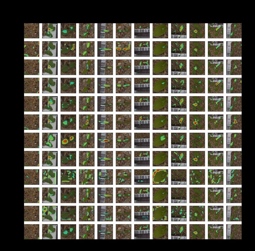
Sensors 2021, 21, 6705                                                                                            2 of 18

                               In physical and chemical methods, weed management is conducted in two steps:
                         capturing images in the field and weed detection/classification [11]. The earlier step can
                         feasibly be carried out through the use of new imaging technologies. In the second step,
                         however, collecting and labeling data is a time-consuming and error-prone procedure,
                         especially in agricultural areas where many different kinds of plants are mixed in [12–14].
                         In artificial neural network (ANN) modeling, it is possible to determine imprecise temporal
                         and spatial parameters [15,16]. Thus, autonomous weed management methods combined
                         with computer vision approaches could help farmers to detect and classify weeds and con-
                         sequently improve weed management and decision-making [17,18]. Thus, the application
                         of an accurate weed classification method plays a critical role in precise farming, helping
                         to determine the weed-combating approach used, maximize crop yields, and improve
                         economical returns [19–22].
                               CNNs have shown promising performance for image classification, including agri-
                         cultural applications. However, one of the main challenges with deep neural networks
                         (DNNs) is the lack of explanation, known as the black-box problem, concerning the human
                         perception of the model’s logic within the classification [23]. Therefore, an interpretable
                         map is an efficient means of explaining the model’s prediction as well as understanding
                         the data better.
                               To mitigate the aforementioned challenges, explainable artificial intelligence (XAI) is
                         proposed to present a better explanation of black-box DNN models [24]. In classification
                         methods based on XAI, the model identifies the class prediction and highlights the critical
                         data content to draw attention to a given decision. Therefore, the models are also called
                         attention models.
                               In agriculture, the model’s explanation map supports a research area called the weed
                         identification key (WIK), which is mainly adopted to discriminate species with a higher
                         accuracy [25]. WIKs assist agronomists in classifying both common and uncommon features
                         between species with an acceptable level of accuracy. Therefore, the model’s transparency
                         helps us to create and understand the WIKs perceived by the model.
                               Positive and negative explanation maps, which explain why a model does or does not
                         classify an image into a corresponding category, introduce both mutual and distinctive per-
                         ceptible features from different classes. The negative explanation is especially informative
                         in classification problems with high similarities between classes, such as in agricultural
                         datasets [26].
                               Conventional WIKs include both positive and negative explanations simultaneously.
                         In computer vision problems, self-attention transformers are utilized to discriminate the
                         locations of objects. According to [27], the slot attention module includes multi-head
                         attention blocks with dynamic weights [28,29]. Slot attention describes the latent features
                         of DNNs by training a set of abstract representations, called slots, for different classes. In a
                         slot attention module, discriminative object regions will be extracted without the need to
                         use humans for supervision. The slot attention, however, will have a low resolution due to
                         the poor resolution of the DNN’s latent features [26].
                               In this paper, two agricultural datasets are employed in the analysis: the Plant
                         Seedlings Dataset (PSD) [30] and the Open Plant Phenotyping Database (OPPD) [31].
                         Both datasets have a weed species-annotated bounding-box for each plant. To improve the
                         resolution of the slot attention with high-level semantics and fine details, a multi-resolution
                         mechanism is adopted here that is based on the slot attention module. Afterwards, to ma-
                         nipulate different feature layers’ impacts on the resulting attention map, a weighted mean
                         approach is used to combine multi-resolution maps regarding their saliency. Three main
                         aspects are used for creating the slot attention in agricultural applications, and the proposed
                         model is evaluated based on them: (1) the resolution of the attention map, (2) the size of
                         the area covering the object, and (3) the features of the weed species that cause the model
                         to not classify the weed as another class (hereafter called negative explanation).
Sensors 2021, 21, 6705 3 of 18
The proposed framework for multi-resolution slot attention and the proposed weighted
average method in this paper are described in Section 2. Then, in Section 3, the results are
elaborated within two different setups. Lastly, the discussion and conclusion are provided
in Sections 4 and 5, respectively.
2. Materials and Methods
2.1. Utilized Datasets
The model was trained and tested with two different datasets to evaluate how well
it could support attention on mutual features. Hence, two plant seedling datasets, PSD
and OPPD, were employed in this paper. Differences in the growing medium were used to
evaluate the proposed model on agricultural datasets with changing settings.
In Table 1, the European and Mediterranean Plant Protection Organization (EPPO)
labels for the species utilized in this paper are shown. Monocot and dicot species are
represented by M and D, respectively, in Table 1.
Table 1. EPPO code and English name of the species utilized in this paper.
EPPO Code English Name Mono/Dicot
ALOMY Black grass M
APESV Loose silky-bent M
BEAVP Sugar beet D
CAPBP Shepherd’s purse D
CHEAL Fat hen D
GALAP Cleavers D
GERMO Small-flowered crane’s bill D
MATIN Scentless mayweed D
SINAR Charlock D
STEME Common chickweed D
TRZAW Common wheat D
ZEAMA Maize M
The PSD contains images of 960 unique plants across 12 plant species in several growth
stages with a ground sampling distance of 10 pixels per mm [30]. The camera (Canon 600D)
was placed at a 110–115 cm distance above the soil surface. Plants in the PSD are grown
indoors with even illumination conditions. The surface of the soil in the PSD is covered
with stones to avoid green indoor moss artifacts and to ease the distinction between plants
and the background. There is no specific plant color variation in the PSD. In the PSD, weed
species are detected and cropped out.
The original OPPD is comprised of 64,292 unique crop plants. These plants include
47 different species in multiple growth stages with a ground sampling distance of 6.6 pixels
per mm [31]. In our work, we only considered growth stages and species that are common
in the PSD. Therefore, 21,653 and 5393 plant images are utilized as training and test
sets here, respectively. Images were illuminated using a ring flash to ensure consistent
light conditions during the image acquisition. The OPPD was able to better capture
the naturally occurring variability in the plant morphology of the species in abnormal
conditions. To meet this goal, plants were grown with different amounts of water and
levels of nutrition stress. As with the PSD, there is only one plant per image for training
and testing the model.
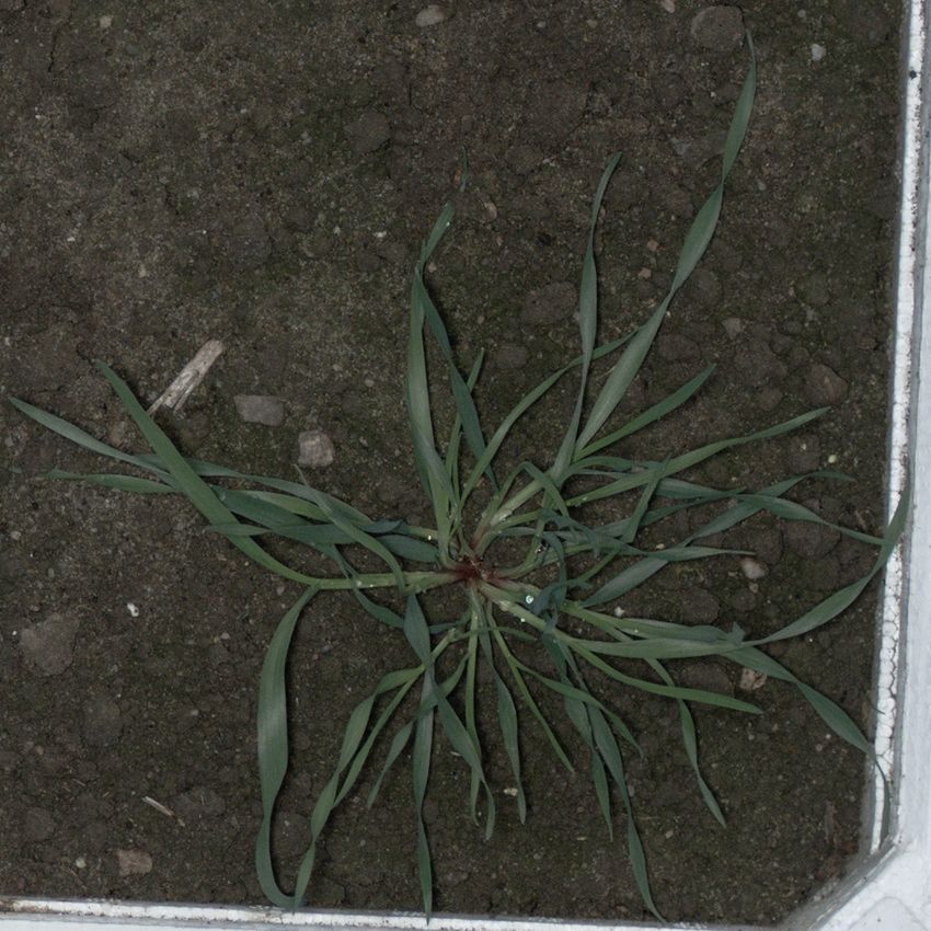
Figure 1 shows different samples from species that are common to both the PSD
and OPPD, respectively. Images are sorted from the left to right according to the growth
stage. Three samples are shown for the OPPD and two for the PSD, since growth stage
diversity is higher in the OPPD. There are multiple images for each plant in the growing
procedure. The images depicted in Figure 1 were resized to a common resolution. Moreover,
the samples in the training and test sets were randomly divided into proportions of 80% and
20%, respectively. The training and test samples were randomly separated for each image.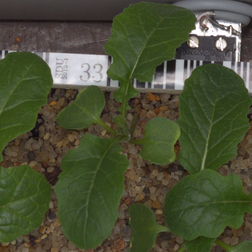
Sensors 2021, 21, 6705                                                                                           4 of 18

                              There are nine mutual species in the PSD and OPPD. Twelve species from the PSD
                         were utilized in experiments when the PSD was employed for both training and testing.
                         Otherwise, only the nine common species of the PSD and OPPD were fed into the network.
                         The two datasets have different illumination conditions. For instance, there is a bright area
                         around the terminal bud in the later growth stages of CHEAL, which is a deterministic
                         feature. However, this feature is more apparent in the OPPD than in the PSD due to
                         the illumination. Therefore, the combination of these two datasets could assist us in
                         finding which features were brought out by the model and whether the absent features
                         were essential.
                              It is necessary to mention that the scale of the images is varied due to the data
                         augmentation technique (explained in Section 2.3) applied to the training set. Therefore,
                         the differences in resolution between the two datasets cause no serious problem. On the
                         other hand, the model’s generalizability was examined under changing light, acquisition,
                         and growth conditions. We recommend that the reader review [30,31] if more details about
                         the data acquisition process used in the PSD and OPPD are required.

                         2.2. Neural Network Architecture
                              The overall framework of the proposed pyramid representation—hereafter called high-
                         resolution attention—was inspired by feature pyramid networks [32,33]. By extracting
                         features from different levels, a high-resolution representation of the attention map was
                         achieved (Figure 2).
                              The RGB input image is passed through a DNN to extract features at multiple depths
                         and spatial resolutions (Figure 2a). The extracted features are then passed through the slot
                         attention module (Figure 2b). The slot attention module mainly consists of a transformer.
                         Ultimately, the extracted attention maps gained for other classes from different resolution
                         levels are merged to obtain the high-resolution attention map as the output.

                         2.2.1. Slot Attention
                              The slot attention is generated based on the feature regions with a great explainability
                         of the class. The impact of different regions is formulated using positional encoding in
                         Figure 2b. In this section, we illustrate not only the attention mechanism utilized [27],
                         but also the method proposed to be used for extracting multi-resolution attention maps.
                              In Figure 2, the features were first extracted from different levels F n of the backbone.
                         n depends on the number of spatial downsampling processes used in the DNN, which
                         was four in the ResNet50 [34] adopted in this study. Then, F n s were individually passed
                         through the slot attention module to extract highlighted regions. Slot attention based on
                         a transformer is an iterative module with K slots, where each slot describes a class in a
                         K-classification problem. Through extracted features and positional encoding, the slots are
                         trained to present maps with a high ability to explain the object. Slots are shown by Sit and
                         randomly initialized using a Gaussian distribution.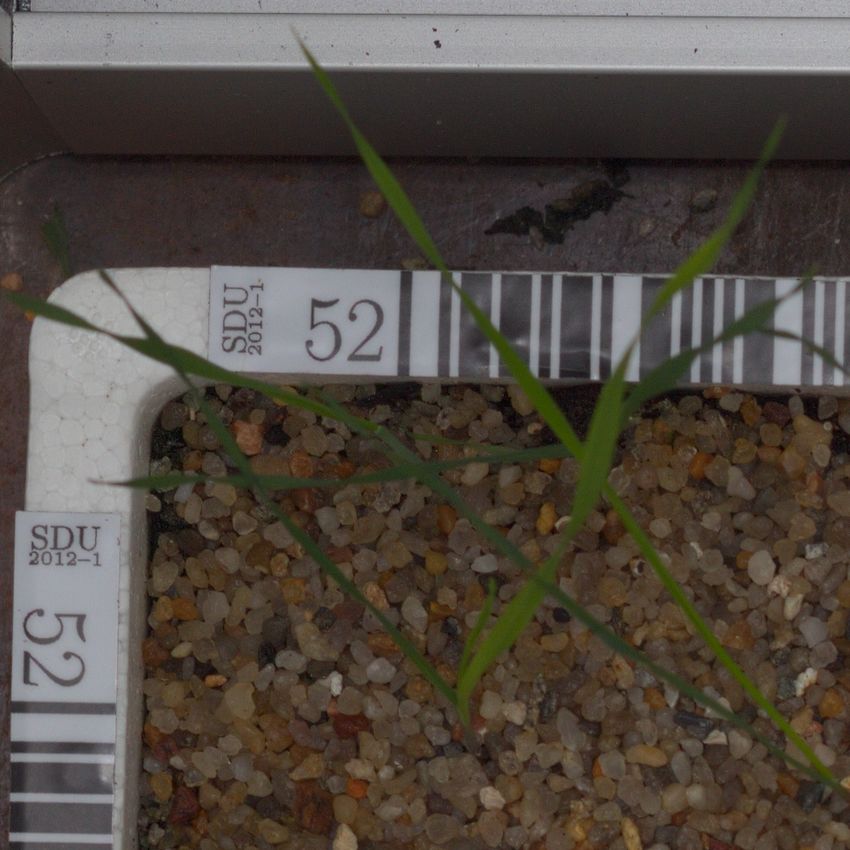
Sensors 2021, 21, 6705                                                                                                     5 of 18

                                     OPPD Dataset                                         PSD Dataset
                   ALOMY
                   SINAR
                   GALAP
                   STEME
                   GERMO
                   CHEAL
                   APESV
                   CAPBP
                   MATIN

      Figure 1. Examples of nine common species from the OPPD and PSD samples during different maturity stages, from left to
      right. OPPD samples were also selected from non-stressed and stressed samples.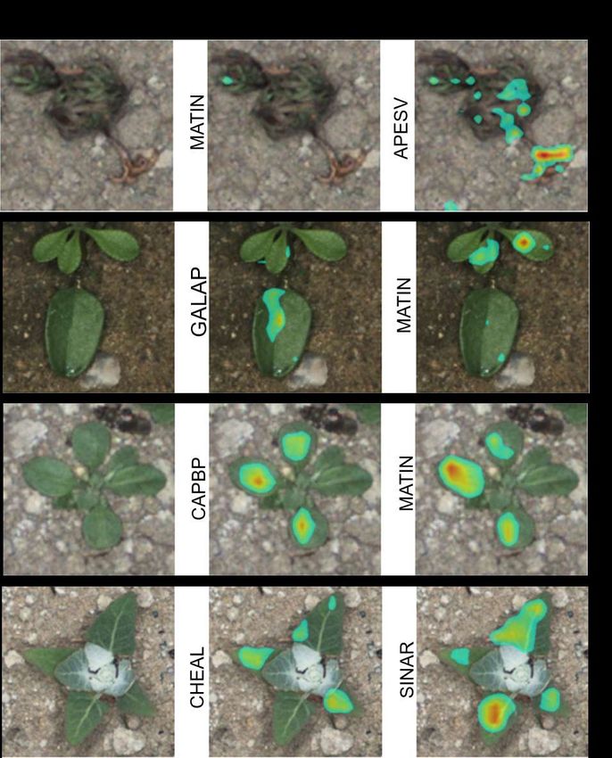
Sensors 21, 6705
2021, 2021,
Sensors 21, 6705 66of
of18
18
(a) (b)
Figure 2. The proposed architecture for plant classification using the slot attention module. (a) The overall architecture for
Figure 2. The proposed architecture for plant classification using the slot attention module. (a) The overall architecture for
extracting features using convolutional blocks (in blue), including obtaining the highlighted attention areas from different
extracting features using convolutional blocks (in blue), including obtaining the highlighted attention areas from different
convolutional blocks and combining multi-resolution slot attention to generate the final attention map (orange blocks).
convolutional blocks and combining multi-resolution slot attention to generate the final attention map (orange blocks).
(b) The slot attention module applied to K-class weed classification using the transformer concept. Slots are depicted as Sit
(b) The slot attention module t
for class i in iteration t. applied to K-class weed classification using the transformer concept. Slots are depicted as Si
for class i in iteration t.
In the multi-head attention block shown in Figure 2, there are three main learnable
In the multi-head
vectors: attention
keys (k), queries block
(q), and shown
values (v)in Figure
[35]. The2,q there
are theare three
slots Sk main
updatedlearnable
within
vectors: keys (k),According
T iterations. queries (q), and the
to [27], values
slots(v) [35].
are The to
trained q are the slots Skprecise
be sufficiently updated within
after three
T iterations.
iterations.According
While q is to [27], the
formed slots
based onare
thetrained to be ksufficiently
labels used, precise
and v are based onafter three
the inputs.
iterations.
The higherWhile is formed
the qsimilarity basedbetween
gained on the qlabels
and kused, and vthe
is, thekbetter aremodel
basedhasonbeen
the inputs.
trained
Thewith
higher the similarity gained between
respect to precision of explanation: q and k is, the better the model has been trained
with respect to precision of explanation:
1
U t+1 =< So f tmax ( √ < k(inputs), q(slots) T >) T , v(inputs) >, (1)
t +1 1 D
U =< So f tmax ( √ < k(inputs), q(slots)T >)T , v(inputs) >, (1)
D
where Equation (1) is the multi-head attention block shown in Figure 2; D is the common
dimension
where Equation space
(1) isbetween three vectors
the multi-head and v shown
q, k, block
attention utilizedinasFigure
a normalization
2; D is the term;
common and
U t+1 is the updated slots obtained in iteration t. The inner product < ., . > of the vectors
dimension space between three vectors q, k, and v utilized as a normalization term; and
U t+is computed
1 is the updated to find the
slots vectors’insimilarities.
obtained iteration t. Softmax
The innerisproduct
then applied to of
< ., . > normalize
the vectorsthe
attention maps and suppress the attention gained for the other
is computed to find the vectors’ similarities. Softmax is then applied to normalize the classes. Then, a gated
recurrent
attention mapsunitand (GRU) is utilized
suppress to updategained
the attention the slotsfor [36]. GRU classes.
the other is a learnable
Then,recurrent
a gated
function that is used for updating slots with the aggregated
recurrent unit (GRU) is utilized to update the slots [36]. GRU is a learnable updates and previous slots.
recurrent
In [27], the investigations show improvements in the model’s performance
function that is used for updating slots with the aggregated updates and previous slots. when a multi-
layerthe
In [27], perceptron (MLP)show
investigations is adopted after the GRU,
improvements in the model’s performance when a multi-
layer perceptron (MLP)t+is 1 adopted after the t GRU,
S = MLP( GRU (S , e · U t+1 )), St = [S1t , S2t , . . . , Skt ], (2)
t +1
where St and StS+1 are MLP
=the ( GRU (and
previous · U t+1 )),slots,
St , eupdated St = respectively.
[S1t , S2t , . . . , STherefore,
t
k ], (2)
all the slots
are updated in each iteration. To easily switch between positive and negative explana-
where St and St+1 are the previous and updated slots, respectively. Therefore, all the slots
tions, the sign parameter e is determined. A comprehensive description of the negative
are updated in each iteration. To easily switch between positive and negative explana-
explanation and Equation (2) is provided in the study of [26].
tions, the sign parameter
Instead e is determined.
of interpolating the last layerAfeatures
comprehensive
to gain andescription
attention map of with
the negative
the same
explanation and Equation
input dimension, (2) is the
we applied provided in the study
slot attention of [26].
after four convolutional blocks in ResNet50.
Instead of interpolating
Afterwards, the lastlayers
slots from different layer with
features to gain
different an attention
resolutions were map with theusing
combined samea
input dimension, we applied the slot attention
fusion rule described in the next section. after four convolutional blocks in ResNet50.
Afterwards, slots from different layers with different resolutions were combined using a
fusion rule
2.2.2. described
Fusion Rule in the next section.
In slot attention, deeper layers have a sparse but high accuracy regarding the object
2.2.2. Fusion Rule
explanation, albeit with a lower spatial resolution. On the other hand, shallower layers
In slot attention, deeper layers have a sparse but high accuracy regarding the object
explanation, albeit with a lower spatial resolution. On the other hand, shallower layers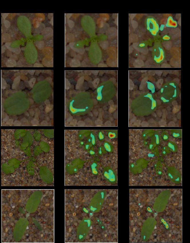
Sensors 2021, 21, 6705                                                                                            7 of 18

                         have a high spatial resolution with a lower accuracy regarding object localization. When
                         combining different layers of slot attention, the degree of certainty should impact the
                         dedicated weight of the fused attention maps. The higher the average values of the slots
                         are, the higher the model’s certainty will be with regard to localization. Therefore, a slot
                         attention map with higher average values should have a higher impact on the fused
                         attention map. The following equation was used for this purpose to combine different
                         layer attention maps:
                                                                   n
                                                                        W
                                                           SF = ∑ n l         · Sl ,                              (3)
                                                                     ∑
                                                                 l =1 j =1
                                                                           Wj

                         where Wl is the summation of elements in the updated slots for the lth layer of the backbone.
                         In other words, the attention map with the highest Wl had the greatest effect on the fused
                         slots S F . In Figure 2, the fusion rule is represented by an orange block. Therefore, the final
                         attention map was formed based on the combination of shallow layers with a high precision
                         and deep layers with a high resolution. The proposed weighted mean approach preserves
                         the highlighted areas through the use of upsampling.

                         2.2.3. Loss
                              Two loss functions were required for this problem: one for the classification and the
                         other for the attention. For the classification, the cross-entropy (LCE ) of the deepest layer
                         of the backbone was computed, ref. [26] presents SCOUTER loss, defining how large the
                         attention area should be through the formula:

                                                            LSCOUTER = LCE + λW,                                     (4)

                         where W is the sum of elements in the slots gained from different backbone layers controlled
                         by the hyperparameter λ. λ is adjusted based on how broad the attention areas are in the
                         specific dataset.

                         2.3. Parameter Setting
                               Input images in both PSD and OPPD have square dimensions. Input images were
                         first resized to 360 × 360 pixels with bilinear interpolation to balance images with different
                         dimensions at different growth stages. Then, ResNet50 [34] was used as the backbone
                         in order to extract the latent features. There are four convolutional blocks in ResNet50.
                         Thus, four slot attention modules were implemented on intermediate features to merge the
                         attention maps created based on their saliency. The model is implemented by PyTorch v1.7.
                         The model was pretrained using ImageNet [37]. The batch size was 32, the initial learning
                         rate was 10−4 , and AdamW [38] was utilized as the optimizer. The attention was shown in
                         positive and negative explanations. In Equation (4), λ was set to 2 in all evaluations based
                         on trial and error. The number of iterations used for the slot attention was set to three.
                         Additionally, the model was trained in 80 epochs. In the training procedure, the model was
                         trained using multiple training processes on four GPUs (48 GB).
                               Translation, rotation, scaling, shear, cut-out, image corruption, Gaussian noise, and
                         color space-changing methods were utilized as data augmentation techniques (color aug-
                         mentation was only employed for generating results in Section 3.3). The translation (along
                         the x and y axes), rotation, scaling, and shear were randomly selected within [−0.1, 0.1]
                         of the input’s dimension, [−10◦ , 10◦ ], [0.8, 1], and [−20◦ , 20◦ ], respectively. Only a few
                         data augmentation methods were randomly applied to the data each time in order to avoid
                         significant variations in the images.

                         3. Results
                              This section is ordered into an exploration of attention maps from different backbone
                         layers, an evaluation of the PSD, and a cross-evaluation of the OPPD and PSD.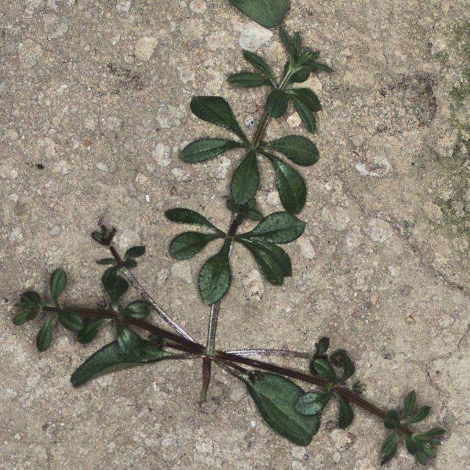
Sensors 2021, 21, 6705                                                                                         8 of 18

                         3.1. Multi-Resolution Attention
                              Figure 3 shows the attention maps gained using three examples from different classes
                         (narrow and broad leaves). The attention map was utilized as the alpha channel, with ar-
                         eas with values close to zero neglected by applying a threshold. The original images
                         are shown to give a better view of where weeds are located. Low-resolution attention
                         was obtained by using only the backbone’s last layer of slot attention. High-resolution
                         attention was obtained by applying the weighted average to the attention maps gained
                         from different levels.

                         Original Image          Low-Resolution Attention High-Resolution Attention

                         Figure 3. Comparison between the low- and high-resolution predicted attention map for three
                         samples from different classes.

                               The attention map gained from only the last layer of the backbone is highly precise in
                         terms of discriminating the salient features of weeds, as shown in the middle column of
                         Figure 3. In the low-resolution attention map, highlighted areas were roughly distributed
                         along the horizontal and vertical axes due to the interpolation (the middle column in
                         Figure 3). Moreover, attention spots in the low-resolution map were not placed precisely
                         on the weed. Contrarily, the high-resolution attention map was distributed smoothly along
                         the plant (the right column in Figure 3).
                               It is worth mentioning that the predicted attention was partly placed on the back-
                         ground in some cases of high-resolution attention (such as the last row in Figure 3). This
                         phenomenon was likely due to the impact of shallower layers on the combined attention
                         map. This result could also be related to noisy backgrounds, blurred features, etc. For ex-
                         ample, in the last row of Figure 3, the high-resolution attention map also points to stones
                         and the box in the background.
                               Additionally, attention maps from different layers on a weed-specific sample are
                         shown in Figure 4. All slots from different layers are scaled up in Figure 4. The two
                         last layers (Figure 4e,f) had an excellent resolution compared with the slot attention from
                         the other layers (Figure 4c,d). Normalized heatmaps from various slots are presented
                         here in order to give a better demonstration of each layer’s attention. The scale bar for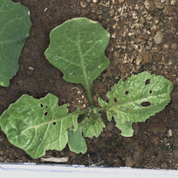
Sensors 2021, 21, 6705 9 of 18
each slot is presented alongside it. It is necessary to mention that the legends are not
directly comparable between figures. The 4th and 3th layers’ weights, referred to as Wl
in Equation (3), were considerably more important than the 2nd and 1st layers. In other
words, while the attention maps extracted from the deeper layers (Figure 4c,d) had a higher
accuracy in identifying plants, the attention maps from shallower layers (Figure 4e,f) had
lower attention weights for the whole image.
(a) (c) (b) (d) (e) (f)
Figure 4. The impact of multi-resolution attention maps. (a) The original image and (b) the weighted averaged attention
map. (c) 4th layer, (d) 3rd layer, (e) 2nd layer, and (f) 1st layer slot attention gained from the backbone layers. The bluish
areas in (b) were filtered to improve the clarity of the visualization.
The weighted average fusion rule provides a balance between accurate, low-resolution
attention from the last layer and inaccurate, high-resolution attention from the first layer.
In Figure 4b, the attention map has a multi-directional explanation from shallower layers
with a high accuracy in detecting weeds from deeper layers simultaneously. Therefore,
the distribution of the attention maps was enhanced and developed to provide precise,
omnidirectional attention maps. The omnidirectional attention map was creating using
high-resolution attention maps from shallower layers.
3.2. Evaluations on the PSD
In this section, all 12 species in the PSD are employed for training and inference.
In Figure 5, the average confusion matrix for the test set is shown for the negative explana-
tion across ten repeats. The negative attention helps us to explicitly understand the data
better. The average is then computed, since the model performance slightly changes for the
random data augmentation and weight initialization. All samples visualized in attention
matrices were selected from correctly classified instances.
$/20<
6,1$5
*$/$3
67(0(
75=$:
7UXHODEHO
$FFXUDF\
&+($/
$3(69
=($0$
0$7,1
&$3%3
*(502
%($93
< 5 3 ( : / 9 $ ,1 3 2 3
$
/$ 6
0 $ 0 $ ( 0 7 % 0 9
,1 ( = ( $ $ 3 $
/2 6 *
$ 7 5 &
+
$
3 ( 0 &
$ (
5
%
(
$ 6 7 = *
3UHGLFWHGODEHO
Figure 5. The average confusion matrix for the negative explanation of the PSD test set with 12 classes. The overall accuracy
gained was 95.42%.
Sensors 2021, 21, 6705                                                                                                        10 of 18

                                       In Figure 5, the average accuracy is 95.42%. The diagonal of the matrix has a more
                                 than 90% accuracy for all samples, except ALOMY. ALOMY and APESV are both monocots
                                 (narrow leaves), and it is hard to discriminate them using an agronomist. Since APESV
                                 comprises more samples than ALOMY, the model presented a clear bias towards misclassi-
                                 fying monocot samples as APESV when the uncertainty is high. Additionally, the model
                                 showed a clear tendency to classify ZEAMA (also monocot) as APESV. However, ZEAMA
                                 has a particular feature in earlier growth stages, making it easier for the model to identify
                                 it than ALOMY. Therefore, the model has a higher certainty for ZEAMA, particularly in the
                                 earlier growth stages.
                                       In Figure 6, the attention confusion for the negative explanation is shown. It is
                                 expected that the highlighted areas will be absent in the diagonal, while the non-diagonal
                                 images will have meaningful distinctive attention areas.

      Figure 6. Negative attention matrix for PSD dataset with 12 classes. Columns are classes and rows are model predictions.
      The attention matrix’s diagonal has remarkably less attention, since the model classifies using the negative loss value in
      Equation (2).
Sensors 2021, 21, 6705 11 of 18
The feature is well represented by the highlighted area, which is used for predicting
APESV for ZEAMA. In Figure 6, the highlighted spots on the background were supposed to
be generated for two reasons: (i) the scale of the stones varied regarding the growth stage
(input images were re-scaled to 360 × 360) and the background had remarkable impacts
in classes with small changes across different growth stages, and (ii) the positive layer’s
weights were on the background while the negative layer’s weights were on the foreground.
The positive confusion matrix is shown in Figure 7, which led to a similar trend as that
for the negative explanation. The non-diagonal predictions for the same class are helpful
for understanding which features were missed in the dataset or which species had higher
similarities that made the model uncertain. Therefore, a high number of doubtful species
were recognized and could be utilized as an alarm in the other field classification.
$/20<
6,1$5
*$/$3
67(0(
75=$:
7UXHODEHO
$FFXUDF\
&+($/
$3(69
=($0$
0$7,1
&$3%3
*(502
%($93
< 5 3 ( : / 9 $ ,1 3 2 3
$
/$ 6
0 $ 0 $ ( 0 7 % 0 9
,1 ( = ( $ $ 3 $
/2 6 *
$ 7 5 &
+
$
3 ( 0 &
$ (
5
%
(
$ 6 7 = *
3UHGLFWHGODEHO
Figure 7. Confusion matrix for the positive explanation of the PSD test set with 12 classes. The average gained accuracy
was 96%. The diagonal with a dark heatmap is desirable.
The same samples in the negative explanation are selected for the positive explanation
in Figure 8. The diagonal attention areas show which part of the plant has a significant
weight in classification during training. In other words, the positive explanation empha-
sizes species patterns that are necessary for the model. In class ZEAMA, for instance,
the highlighted area shows the particular part that is unique in the class and not the whole
leaf. Comparing Figure 7 with Figure 5, it can be seen that the accuracy of the class ZEAMA
improved by approximately 9% from the negative to the positive explanation. The reason
for this was that ZEAMA has similarities to both monocots and dicots (broadleaves). As a
result, it was simpler for the network to reveal the unique feature for ZEAMA (in Figure 8)
in the negative explanation (in Figure 6). This also reveals the accuracy improvement from
the negative to positive explanation.
In Figure 8, the model came with different parts of plants in different classes or growth
stages, depending on the similarities between species. For instance, while the model’s
attention was on the whole leaves for GALAP, as an example of a case that is difficult to
classify during early growth stages, the main attention was on the center of the plant for
CAPBP, as an example of a case that is easier to classify in the later growth stages.Sensors 2021, 21, 6705 12 of 18
Figure 8. The positive attention matrix for the PSD test set with 12 classes. The diagonal images bold out the particular
features that the model uses for the classification.
3.3. Evaluations on PSD and OPPD
In this section, the model was trained on the PSD and inferenced on the OPPD as
a cross-dataset evaluation. In Figure 9, eight misclassified samples are shown through
cross-dataset evaluation. For each sample, correct and predicted positive attention maps
are depicted on the original image. The label for each slot attention is presented on the
left side of the image. Four class species are shown for two cross-dataset evaluations:
(i) in Figure 9a, the model was trained on the OPPD and evaluated on the PSD, while (ii) in
Figure 9b the model was trained on the PSD and tested on the OPPD.
Classes CAPBP and MATIN look similar in their earlier growth stages, which made
prediction harder. Furthermore, samples of stressed species from the OPPD were misclassi-
fied in most cases. For instance, a stressed sample from class MATIN is shown in Figure 9b
from the OPPD which was predicted as class APESV.Sensors 2021, 21, 6705 13 of 18
In Table 2, a comparison between the use of the proposed method and state-of-the-
art methods on the PSD and OPPD is shown. The proposed method in this study was
evaluated with both a positive explanation, Ours+, and a negative explanation, Ours−.
For the PSD, two other state-of-the-art methods are compared in Table 2.
(a) PSD (b) OPPD
Figure 9. Misclassified samples in cross-dataset evaluation. In (a), the model was trained on the OPPD with positive
attention, while the inference was trained on the PSD. Conversely, in (b), the model was trained on the PSD with positive
attention, while the inference was trained on the OPPD.
Table 2. The comparison between the use of multi-resolution attention on the PSD and OPPD test
sets with the state-of-the-art methods.
Dataset Accuracy (%) Parameters (M)
EffNet [39] OPPD 95.44 7.8
ResNet50 [40] OPPD 95.23 25
Ours− OPPD 95.42 23.98
Ours+ OPPD 96.00 23.98
SE-Module [41] PSD 96.32 1.79
Ours− PSD 97.78 23.54
Ours+ PSD 97.83 23.54
In Table 2, the proposed method was found to outperform the previous methods in
both OPPD and PSD evaluations, ref. [39] conducted the training with a five-fold cross-
validation of the PSD using EfficientNet. The number of parameters used was lower in our
methods (the negative and positive attention models) in spite of the use of the multiple
slot attention module, since the fully connected layer is omitted. However, the numberSensors 2021, 21, 6705 14 of 18
of parameters utilized in [41] is considerably lower than that in the attention method
proposed in this paper.
The OPPD was published quite recently and only one applied method is given as
a comparison in Table 2. In the OPPD study conducted by [41], the SE-module is imple-
mented for classification. The SE-module is a multi-scale fusion approach that does not
utilize attention. The proposed method outperformed the method described in the study
by [41] in terms of accuracy.
Instances from different growth stages of the class CHEAL are presented in Table 3 to
emphasize the importance of contrast and color space in classification. The result in Table 3
was gained by a model that had been both trained and tested on the OPPD. In the first
growth stage, attention was also paid to leaves (the last row). However, the attention was
attracted to the center in later growth stages (the first and middle rows).
Table 3. Positive and negative explanation of the class CHEAL by the model trained and tested on the OPPD dataset. Images
are sorted in order of increasing growth stage. The model had different highlighted areas and understandings of CHEAL in
different growth stages.
Original Image Positive Attention Negative Attention
ALOMY SINAR GALAP STEME GERMO APESV CAPBP MATIN
The impact of growth stage on CHEAL is shown in Table 3. In the OPPD, the class
CHEAL was a prominent feature in the later growth stages; there are white hairs on the
leaves that are more obvious in the center of plants. In the PSD, however, the whitish
domain is less visible due to the different brightness and contrast. Therefore, the atten-
tion gained from the training and inference with the PSD and the OPPD, respectively,
highlighted areas over leaves, not over stems.
The model shows the leaves for monocot species in Table 3—i.e., ALOMY and
MATIN—since the broad leaves are distinctive areas in the later growth stages. For dicot
species, the white center area gained the model’s attention.
4. Discussion
The proposed model presented a high-resolution attention map of weed species; the
map enabled us to better perceive the model’s decision [42]. In the previous transformer-
based methods, the resolution of the attention map was low due to the interpolation
applied for resizing the attention map from 12 × 12 to 360 × 360 [43]. This challenge was
mitigated in the approach proposed in this paper by providing a multi-layer attention
mechanism. In general, the model has a lower certainty regarding attention in the first
few layers [44,45], but its precision is higher. Therefore, the proposed algorithm merged
multi-layer attention maps from different layers to generate a precise high-resolution
representation that included principle features for weed discrimination.Sensors 2021, 21, 6705 15 of 18
The positive explanation maps help us to differentiate weed species during the early
growth stages and are frequently utilized in transformers [42,46]. Moreover, the negative
explanation maps support the model’s classification, particularly during the mature growth
stages, where the dissimilarities between species are substantial [26]. Moreover, the model’s
uncertainty should help farmers to decide which species should be reconsidered during
weed management [47].
In terms of statistical comparison, the proposed model outperformed the state-of-the-
art methods using positive attention, as illustrated in Table 2. The performances of the
proposed model showed slight improvements compared with those shown in the study
by [40]. This is likely due to the attention explanation, better data augmentation, tuning
of the hyper-parameters, etc. The attention loss also showed improvements in terms of
classification for the positive and negative explanations of the PSD.
The model’s challenges in cross-dataset evaluation (Section 3.3) showed that a model
applied to one agricultural dataset might not be robust on the other datasets [48]. The pro-
posed model presented interpretable information about the differences between the two
datasets, which made the model unable to classify properly. Moreover, only diversity
was not sufficient to improve the performance, since the model that was trained with the
OPPD and had a wider variety still struggled when applied to the PSD. Nevertheless,
the proposed method should help us determine what areas showed significant differences
between the two datasets. Therefore, there should be a better explanation as to why the
model achieved a lower accuracy during the classification. The cross-dataset evaluation
also highlighted the necessity of understanding the data better during the training and test
phases in DNNs.
In the cross-dataset evaluation, three characteristics that will be considered in future
research were not taken into account:
1. Growth stage;
2. Partial or heavy occlusion;
3. Partial plant appearance.
The model’s performance is expected to be improved when a growth stage label is
also given to the model due to species variation in different growth stages [13,49]. Fur-
thermore, two critical factors observed from Figure 9 were the impact of occlusion and
partial appearance due to the classification. For instance, class GALAP showed a partial
appearance in Figure 9b (where only half of the plant is visualized), while class CAPBP
showed partial occlusion due to the neighboring plant in Figure 9a. A great quantity of
real in-field annotated images would support our knowledge about the model’s perfor-
mance regarding the existence of occlusion, stress, neighboring plants, etc. In conclusion,
the characteristics mentioned above should be investigated in future research.
5. Conclusions
In this paper, a high-resolution attention architecture was proposed in order to improve
the resolution and location of highlighted weed areas in weed management. The resulting
explanation is a foolproof approach for interpreting the similarities and dissimilarities
between different weed species through automated weed control. By understanding the
black-box model better, we were able to gain more transparency regarding the model’s
classification of different weed species through maturation. Therefore, self-attention maps
from different layers of a ResNet model were extracted to improve the attention precision.
The proposed method was able to simultaneously preserve the accuracy from deeper layers
and develop the resolution using shallower layers. In addition, this explanation is useful
when studying the generalizability of a model for cross-dataset evaluations. The proposed
precise and high-resolution attention map was able to explain the datasets better in terms
of their visual aspect. Furthermore, the high-resolution attention map highlighted different
patterns in a species through various growth stages. The influence of growth stage on
attention maps through weed classification is a matter that should be investigated in
future studies.Sensors 2021, 21, 6705 16 of 18
Author Contributions: Conceptualization, R.N.J.; methodology, S.F. and S.K.S.; software, S.F.; formal
analysis, S.F., S.K.S. and R.N.J.; writing—review and editing, S.F., S.K.S., M.D. and H.K.; visualization,
S.F. and S.K.S.; supervision, R.N.J. and H.K.; funding acquisition, R.N.J. All authors have read and
agreed to the published version of the manuscript.
Funding: This research was funded by the Green Development and Demonstration Program (GUDP)
under the Danish Ministry for Food, Agriculture, and Fisheries (project: Square Meter Farming
(SqM-Farm), journal number: 34009-17-1303).
Institutional Review Board Statement: Not applicable.
Informed Consent Statement: Not applicable.
Data Availability Statement: Publicly available datasets were analyzed in this study. The data [30,31]
can be found from: https://vision.eng.au.dk/plant-seedlings-dataset/ and https://gitlab.au.dk/
AUENG-Vision/OPPD, accessed on 17 September 2021, respectively.
Conflicts of Interest: The authors declare no conflict of interest.
Abbreviations
The following abbreviations are used in this paper:
CNN Convolutional neural network
D Dicot
DNN Deep neural network
EPPO European and Mediterranean Plant Protection Organization
GRU Gated recurrent unit
M Monocot
MLP Multi-layer perceptron
OPPD Open Plant Phenotyping Dataset
PSD Plant Seedlings Dataset
ReLU Rectified linear unit
WIK Weed identification key
XAI Explainable artificial intelligence
References
1. Singh, C.B. Grand Challenges in Weed Management. Front. Agron. 2020, 1. [CrossRef]
2. Sharma, A.; Shukla, A.; Attri, K.; Kumar, M.; Kumar, P.; Suttee, A.; Singh, G.; Barnwal, R.P.; Singla, N. Global trends in pesticides:
A looming threat and viable alternatives. Ecotoxicol. Environ. Saf. 2020, 201, 110812. [CrossRef]
3. Abbas, T.; Zahir, Z.A.; Naveed, M. Field application of allelopathic bacteria to control invasion of little seed canary grass in wheat.
Environ. Sci. Pollut. Res. 2021, 28, 9120–9132. [CrossRef]
4. Ren, W.; Banger, K.; Tao, B.; Yang, J.; Huang, Y.; Tian, H. Global pattern and change of cropland soil organic carbon during
1901–2010: Roles of climate, atmospheric chemistry, land use and management. Geogr. Sustain. 2020, 1, 59–69. [CrossRef]
5. Maggipinto, M.; Beghi, A.; McLoone, S.; Susto, G. DeepVM: A Deep Learning-based Approach with Automatic Feature Extraction
for 2D Input Data Virtual Metrology. J. Process. Control 2019, 84, 24–34. [CrossRef]
6. Bručienė, I.; Aleliūnas, D.; Šarauskis, E.; Romaneckas, K. Influence of Mechanical and Intelligent Robotic Weed Control Methods
on Energy Efficiency and Environment in Organic Sugar Beet Production. Agriculture 2021, 11, 449. [CrossRef]
7. Veeranampalayam Sivakumar, A.N.; Li, J.; Scott, S.; Psota, E.; Jhala, A.J.; Luck, J.D.; Shi, Y. Comparison of object detection
and patch-based classification deep learning models on mid-to late-season weed detection in UAV imagery. Remote Sens. 2020,
12, 2136. [CrossRef]
8. Olsen, A. Improving the Accuracy of Weed Species Detection for Robotic Weed Control in Complex Real-Time Environments.
Ph.D. Thesis, James Cook University, Queensland, Australia, 2020.
9. Schwarzländer, M.; Hinz, H.L.; Winston, R.; Day, M. Biological control of weeds: An analysis of introductions, rates of
establishment and estimates of success, worldwide. BioControl 2018, 63, 319–331. [CrossRef]
10. Gonzalez-de Santos, P.; Ribeiro, A.; Fernandez-Quintanilla, C.; Lopez-Granados, F.; Brandstoetter, M.; Tomic, S.; Pedrazzi, S.;
Peruzzi, A.; Pajares, G.; Kaplanis, G.; et al. Fleets of robots for environmentally-safe pest control in agriculture. Precis. Agric.
2017, 18, 574–614. [CrossRef]
11. Awan, A.F. Multi-Sensor Weed Classification Using Deep Feature Learning. Ph.D. Thesis, Australian Defence Force Academy,
Canberra, Australia, 2020.
12. Dyrmann, M.; Mortensen, A.K.; Midtiby, H.S.; Jørgensen, R.N. Pixel-wise classification of weeds and crops in images by using
a Fully Convolutional neural network. In Proceedings of the International Conference on Agricultural Engineering, Aarhus,
Denmark, 26–29 June 2016.Sensors 2021, 21, 6705 17 of 18
13. Skovsen, S.; Dyrmann, M.; Mortensen, A.K.; Laursen, M.S.; Gislum, R.; Eriksen, J.; Farkhani, S.; Karstoft, H.; Jorgensen, R.N.
The GrassClover Image Dataset for Semantic and Hierarchical Species Understanding in Agriculture. In Proceedings of the
IEEE/CVF Conference on Computer Vision and Pattern Recognition (CVPR) Workshops, Seattle, WA, USA, 14–19 June 2019.
14. Lu, Y.; Young, S. A survey of public datasets for computer vision tasks in precision agriculture. Comput. Electron. Agric. 2020,
178, 105760. [CrossRef]
15. Wang, Y.; Fang, Z.; Wang, M.; Peng, L.; Hong, H. Comparative study of landslide susceptibility mapping with different recurrent
neural networks. Comput. Geosci. 2020, 138, 104445. [CrossRef]
16. Rai, A.K.; Mandal, N.; Singh, A.; Singh, K.K. Landsat 8 OLI Satellite Image Classification Using Convolutional Neural Network.
Procedia Comput. Sci. 2020, 167, 987–993. [CrossRef]
17. Castañeda-Miranda, A.; Castaño-Meneses, V.M. Internet of things for smart farming and frost intelligent control in greenhouses.
Comput. Electron. Agric. 2020, 176, 105614. [CrossRef]
18. Büyükşahin, Ü.Ç.; Ertekin, Ş. Improving forecasting accuracy of time series data using a new ARIMA-ANN hybrid method and
empirical mode decomposition. Neurocomputing 2019, 361, 151–163. [CrossRef]
19. Farkhani, S.; Skovsen, S.K.; Mortensen, A.K.; Laursen, M.S.; Jørgensen, R.N.; Karstoft, H. Initial evaluation of enriching satellite
imagery using sparse proximal sensing in precision farming. In Proceedings of the Remote Sensing for Agriculture, Ecosystems,
and Hydrology XXII, London, UK, 20–25 September 2020; SPIE: Bellingham, WA, USA, 2020; Volume 11528, pp. 58–70.
20. Jiang, H.; Zhang, C.; Qiao, Y.; Zhang, Z.; Zhang, W.; Song, C. CNN feature based graph convolutional network for weed and crop
recognition in smart farming. Comput. Electron. Agric. 2020, 174, 105450. [CrossRef]
21. Sharma, A.; Jain, A.; Gupta, P.; Chowdary, V. Machine learning applications for precision agriculture: A comprehensive review.
IEEE Access 2020, 9, 4843–4873. [CrossRef]
22. Hasan, A.M.; Sohel, F.; Diepeveen, D.; Laga, H.; Jones, M.G. A survey of deep learning techniques for weed detection from
images. Comput. Electron. Agric. 2021, 184, 106067. [CrossRef]
23. Chandra, A.L.; Desai, S.V.; Guo, W.; Balasubramanian, V.N. Computer vision with deep learning for plant phenotyping in
agriculture: A survey. arXiv 2020, arXiv:2006.11391.
24. Masuda, K.; Suzuki, M.; Baba, K.; Takeshita, K.; Suzuki, T.; Sugiura, M.; Niikawa, T.; Uchida, S.; Akagi, T. Noninvasive Diagnosis
of Seedless Fruit Using Deep Learning in Persimmon. Hortic. J. 2021, 90, 172–180. [CrossRef]
25. Leggett, R.; Kirchoff, B.K. Image use in field guides and identification keys: Review and recommendations. AoB Plants 2011,
2011, plr004. [CrossRef] [PubMed]
26. Li, L.; Wang, B.; Verma, M.; Nakashima, Y.; Kawasaki, R.; Nagahara, H. SCOUTER: Slot attention-based classifier for explainable
image recognition. arXiv 2020, arXiv:2009.06138.
27. Locatello, F.; Weissenborn, D.; Unterthiner, T.; Mahendran, A.; Heigold, G.; Uszkoreit, J.; Dosovitskiy, A.; Kipf, T. Object-centric
learning with slot attention. arXiv 2020, arXiv:2006.15055.
28. Vaswani, A.; Shazeer, N.; Parmar, N.; Uszkoreit, J.; Jones, L.; Gomez, A.N.; Kaiser, L.; Polosukhin, I. Attention is all you need.
arXiv 2017, arXiv:1706.03762.
29. Han, K.; Wang, Y.; Chen, H.; Chen, X.; Guo, J.; Liu, Z.; Tang, Y.; Xiao, A.; Xu, C.; Xu, Y.; et al. A Survey on Visual Transformer.
arXiv 2020, arXiv:2012.12556.
30. Giselsson, T.M.; Dyrmann, M.; Jørgensen, R.N.; Jensen, P.K.; Midtiby, H.S. A Public Image Database for Benchmark of Plant
Seedling Classification Algorithms. arXiv 2017, arXiv:1711.05458.
31. Madsen, S.L.; Mathiassen, S.K.; Dyrmann, M.; Laursen, M.S.; Paz, L.C.; Jørgensen, R.N. Open Plant Phenotype Database of
Common Weeds in Denmark. Remote Sens. 2020, 12, 1246. [CrossRef]
32. Lin, T.Y.; Dollár, P.; Girshick, R.; He, K.; Hariharan, B.; Belongie, S. Feature pyramid networks for object detection. In Proceedings
of the IEEE Conference on Computer Vision and Pattern Recognition, Honolulu, HI, USA, 21–26 July 2017; pp. 2117–2125.
33. Zhao, Q.; Sheng, T.; Wang, Y.; Tang, Z.; Chen, Y.; Cai, L.; Ling, H. M2det: A single-shot object detector based on multi-level feature
pyramid network. In Proceedings of the AAAI Conference on Artificial Intelligence, Honolulu, HI, USA, 27 January–1 February
2019; Volume 33, pp. 9259–9266.
34. He, K.; Zhang, X.; Ren, S.; Sun, J. Deep residual learning for image recognition. In Proceedings of the IEEE Conference on
Computer Vision and Pattern Recognition, Las Vegas, NV, USA, 27–30 June 2016; pp. 770–778.
35. Vyas, A.; Katharopoulos, A.; Fleuret, F. Fast transformers with clustered attention. arXiv 2020, arXiv:2007.04825.
36. Yu, Y.; Si, X.; Hu, C.; Zhang, J. A review of recurrent neural networks: LSTM cells and network architectures. Neural Comput.
2019, 31, 1235–1270. [CrossRef] [PubMed]
37. Deng, J.; Dong, W.; Socher, R.; Li, L.J.; Li, K.; Fei-Fei, L. ImageNet: A Large-Scale Hierarchical Image Database. In Proceedings of
the 2009 IEEE Conference on Computer Vision and Pattern Recognition, Miami, FL, USA, 20–25 June 2009.
38. Loshchilov, I.; Hutter, F. Decoupled weight decay regularization. arXiv 2017, arXiv:1711.05101.
39. Ofori, M.; El-Gayar, O. An Approach for Weed Detection Using CNNs And Transfer Learning. In Proceedings of the 54th Hawaii
International Conference on System Sciences, Hawaii, HI, USA, 5–8 January 2021; p. 888.
40. Gupta, K.; Rani, R.; Bahia, N.K. Plant-Seedling Classification Using Transfer Learning-Based Deep Convolutional Neural
Networks. Int. J. Agric. Environ. Inf. Syst. 2020, 11, 25–40. [CrossRef]
41. Haoyu, L.; Rui, F. Weed Seeding Recognition Based on Multi-Scale Fusion Convolutional Neutral Network. Comput. Sci. Appl.
2020, 10, 2406.Sensors 2021, 21, 6705 18 of 18
42. Zhang, P.; Dai, X.; Yang, J.; Xiao, B.; Yuan, L.; Zhang, L.; Gao, J. Multi-scale vision longformer: A new vision transformer for
high-resolution image encoding. arXiv 2021, arXiv:2103.15358.
43. Caron, M.; Touvron, H.; Misra, I.; Jégou, H.; Mairal, J.; Bojanowski, P.; Joulin, A. Emerging properties in self-supervised vision
transformers. arXiv 2021, arXiv:2104.14294.
44. Tian, C.; Xu, Y.; Li, Z.; Zuo, W.; Fei, L.; Liu, H. Attention-guided CNN for image denoising. Neural Netw. 2020, 124, 117–129.
[CrossRef]
45. Chen, G.; Li, C.; Wei, W.; Jing, W.; Woźniak, M.; Blažauskas, T.; Damaševičius, R. Fully convolutional neural network with
augmented atrous spatial pyramid pool and fully connected fusion path for high resolution remote sensing image segmentation.
Appl. Sci. 2019, 9, 1816. [CrossRef]
46. Tay, Y.; Dehghani, M.; Aribandi, V.; Gupta, J.; Pham, P.; Qin, Z.; Bahri, D.; Juan, D.C.; Metzler, D. Omninet: Omnidirectional
representations from transformers. arXiv 2021, arXiv:2103.01075.
47. Brdar, M.; Brdar-Szabó, R.; Perak, B. Separating (non-) figurative weeds from wheat. In Figurative Meaning Construction in
Thought and Language; John Benjamins Publishing Company: Amsterdam, The Netherlands, 2020; pp. 46–70. Available online:
https://benjamins.com/catalog/ftl.9.02brd (accessed on 17 September 2021).
48. Saikawa, T.; Cap, Q.H.; Kagiwada, S.; Uga, H.; Iyatomi, H. AOP: An anti-overfitting pretreatment for practical image-based
plant diagnosis. In Proceedings of the 2019 IEEE International Conference on Big Data (Big Data), Los Angeles, CA, USA,
9–12 December 2019; pp. 5177–5182.
49. Takahashi, Y.; Dooliokhuu, M.; Ito, A.; Murata, K. How to Improve the Performance of Agriculture in Mongolia by ICT. Applied
Studies in Agribusiness and Commerce. Ph.D. Thesis, University of Debrecen, Debrecen, Hungary, 2019.You can also read