Contribution of potential evaporation forecasts to 10-day streamflow forecast skill for the Rhine River - HESS
←
→
Page content transcription
If your browser does not render page correctly, please read the page content below
Hydrol. Earth Syst. Sci., 23, 1453–1467, 2019
https://doi.org/10.5194/hess-23-1453-2019
© Author(s) 2019. This work is distributed under
the Creative Commons Attribution 4.0 License.

Contribution of potential evaporation forecasts to
10-day streamflow forecast skill for the Rhine River
Bart van Osnabrugge1,2 , Remko Uijlenhoet2 , and Albrecht Weerts1,2
1 Deltares,   Operational Water Management Department, Delft, the Netherlands
2 Wageningen    University, Hydrology and Quantitative Water Management Group, Wageningen, the Netherlands

Correspondence: Bart van Osnabrugge (bart.vanosnabrugge@deltares.nl)

Received: 26 September 2018 – Discussion started: 24 October 2018
Revised: 8 February 2019 – Accepted: 24 February 2019 – Published: 14 March 2019

Abstract. Medium-term hydrologic forecast uncertainty is          also for most models similar to the HBV concept and for
strongly dependent on the forecast quality of meteorological      moderate climate zones.
variables. Of these variables, the influence of precipitation        As a by-product, this research resulted in gridded datasets
has been studied most widely, while temperature, radiative        for temperature, radiation and potential evaporation based on
forcing and their derived product potential evapotranspira-       the Makkink equation for the Rhine basin. The datasets have
tion (PET) have received little attention from the perspective    a spatial resolution of 1.2×1.2 km and an hourly time step for
of hydrological forecasting. This study aims to fill this gap     the period from July 1996 through 2015. This dataset com-
by assessing the usability of potential evaporation forecasts     plements an earlier precipitation dataset for the same area,
for 10-day-ahead streamflow forecasting in the Rhine basin,       period and resolution.
Europe. In addition, the forecasts of the meteorological vari-
ables are compared with observations.
   Streamflow reforecasts were performed with the daily
wflow_hbv model used in previous studies of the Rhine us-         1   Introduction
ing the ECMWF 20-year meteorological reforecast dataset.
Meteorological forecasts were compared with observed rain-        Hydrologic forecasting has the aim of predicting the future
fall, temperature, global radiation and potential evaporation     state of important hydrologic fluxes, most notably stream-
for 148 subbasins. Secondly, the effect of using PET clima-       flow. Throughout the process of forecasting, from model
tology versus using observation-based estimates of PET was        setup via initial state estimation to forecast run, meteorolog-
assessed for hydrological state and for streamflow forecast       ical forcing is a key component. Precipitation is known to
skill.                                                            be the main driver of hydrological processes, and most of
   We find that (1) there is considerable skill in the ECMWF      the forecast uncertainty is attributed to inaccurate precipita-
reforecasts to predict PET for all seasons, and (2) using dy-     tion forcing (Cuo et al., 2011; Pappenberger et al., 2005). As
namical PET forcing based on observed temperature and             a consequence, most attention has been given to the accu-
satellite global radiation estimates results in lower evapo-      racy of precipitation forecasts. See for example the review of
ration and wetter initial states, but (3) the effect on fore-     Cloke and Pappenberger (2009).
casted 10-day streamflow is limited. Implications of this find-      Evaporation is a result of the interaction between mete-
ing are that it is reasonable to use meteorological forecasts     orological forcing and physical and physiological processes
to forecast potential evaporation and use this is in medium-      at the land surface. Meteorological forcing provides the po-
range streamflow forecasts. However, it can be concluded          tential energy (potential evaporation or PET) for evaporative
that an approach using PET climatology is also sufficient,        processes to take place. There are many formulas to esti-
most probably not only for the application shown here, but        mate the potential energy available for evaporation, which
                                                                  can be divided in three types of formulas based on their

Published by Copernicus Publications on behalf of the European Geosciences Union.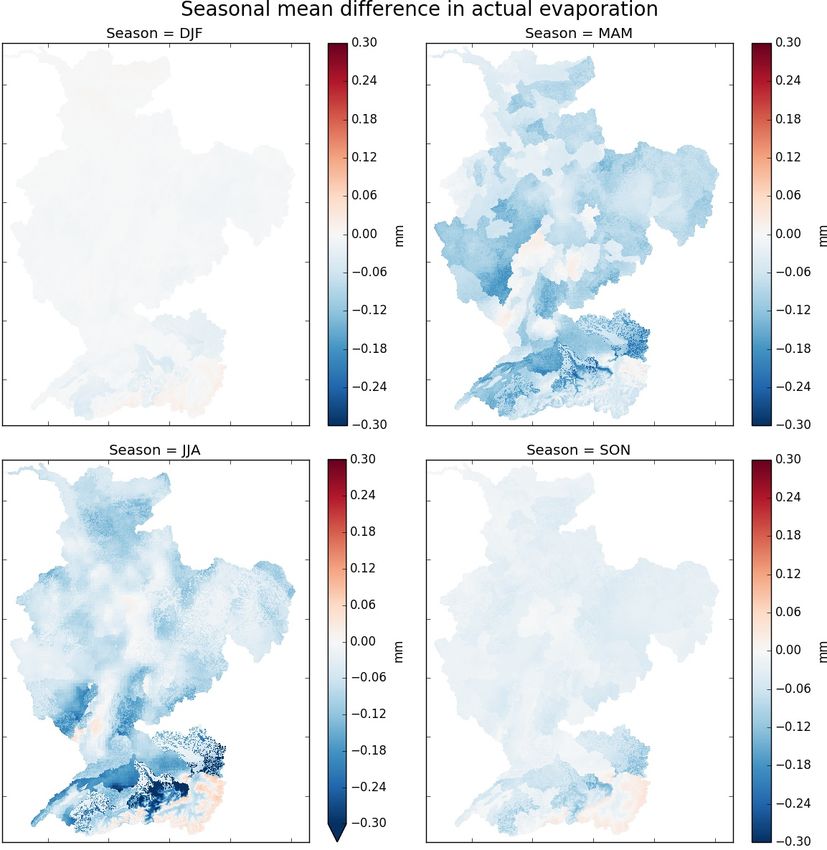
1454                                                 B. van Osnabrugge et al.: Contribution of PET to 10-day forecast skill

data requirements (Xystrakis and Matzarakis, 2011; Xu and         on model results. Recently, van Osnabrugge et al. (2017) de-
Singh, 2002): temperature-based (e.g., Hargreave’s equation,      veloped a high-resolution hourly precipitation dataset for use
Hammon’s equation), radiation-based, and combined meth-           with gridded hydrologic models.
ods (e.g., Hansen’s equation, Turc’s equation, Makkink’s             To answer the research question, model experiments are
equation). From an operational viewpoint the different types      performed, but first the data and hydrological model are
of formulas result in different demands on data availability.     presented (Sect. 2). Second, the model experiments are de-
   Constraints on data availability have led to additional ap-    scribed, which also partitions the main question into three
proximations for potential evaporation. A common approxi-         subquestions (Sect. 3) which are subsequently answered
mation is the calculation of a monthly potential evaporation      (Sect. 4). The paper concludes with a discussion on the re-
climatology or PET demand curves (Bowman et al., 2016).           sults in the wider context of evaporation modeling in hydro-
This climatology is then used as a driver for both historic       logic forecasting and the conclusions (Sect. 5).
potential evaporation and future potential evaporation.
   Hydrological models have proven to be insensitive to
the difference between variable potential evaporation forc-       2     Data and model
ing and climatological monthly potential evaporation forc-
                                                                  Observational data have been preprocessed for use with a
ing with respect to the model’s potential to estimate stream-
                                                                  grid-based hydrological model. The data were processed
flow after calibration (Andréassian et al., 2004; Oudin et al.,
                                                                  with hourly time resolution, on a 1.2×1.2 km grid spatial res-
2005a; Oudin et al., 2005b). However, in forecasting, differ-
                                                                  olution, and for the period mid 1996 through 2015. All source
ent choices in the handling of forcing data can be made be-
                                                                  data to derive the gridded estimates come from sources that
tween the historic update step and the forecast step, while the
                                                                  supply their data in near real time, making the datasets suit-
hydrological model, as a rule, remains the same. It therefore
                                                                  able for operational forecasting. For this study all data were
remains relevant to understand how a single model reacts to
                                                                  aggregated to a daily time step. The hourly datasets are
potential evaporation forcing. Insensitivity to the type of po-
                                                                  downloadable through the 4TU data center (van Osnabrugge,
tential evaporation during the process of calibration does not
                                                                  2017, 2018).
mean that a model is insensitive to the form of potential evap-
oration input.                                                    2.1    Precipitation
   As mentioned above, there has been little attention to the
forecast skill of the secondary forcing variables temperature     For this study the precipitation dataset from van Osnabrugge
and radiation in the hydrological context of potential evapo-     (2017) is used. The precipitation dataset has been derived us-
ration. Furthermore, there is an easy and often used practice     ing the genRE interpolation method based on ground mea-
of avoiding potential evaporation forecasts by using a poten-     surements and the HYRAS (Rauthe et al., 2013) climatolog-
tial evaporation climatology. Therefore, the objective of this    ical precipitation dataset (van Osnabrugge et al., 2017).
study is to assess to what extent potential evaporation fore-
casts can contribute to streamflow forecast skill.                2.2    Temperature
   This question is evaluated for the Rhine basin in Eu-
rope (Fig. 1). The Rhine is one of the basins currently em-       Temperature observations (1996–2016) are interpolated on
ployed as a case study for the IMproving PRedictions of           the same 1.2 × 1.2 km grid as the precipitation data. Temper-
EXtremes (IMPREX) project, which aims to improve pre-             ature is derived from interpolation of ground measurements
dictions and management of hydrological extremes through          with correction for elevation using the SRTM digital eleva-
climate services (van den Hurk et al., 2016).                     tion model (Farr et al., 2007) and standard lapse rate as fol-
   Several studies already directly addressed some aspects        lows.
of operational ensemble flow forecasts in the Rhine. Renner          To calculate temperature Tx at a given grid cell x from a
et al. (2009) showed that at the time meaningful hydrologi-       number of n surrounding stations, determine a set of weights
cal ensemble forecasts could be produced up to a 9-day lead       based on inverse-distance squared weighting between all sta-
time for the Rhine River based on ECMWF ensemble mete-            tions (typically the n closest stations) and the grid cell. This
orological forecasts. Reggiani et al. (2009) used a Bayesian      step can have a threshold for maximum distance. di,x is the
ensemble uncertainty processor to improve the assessment          distance between station i and cell x:
of uncertainty in the ensemble forecast. Terink et al. (2010)                1
                                                                             2
                                                                            di,x
applied downscaling techniques to ERA15 ECMWF reanal-
                                                                  wi,x =   n            .                                      (1)
ysis data to develop a downscaling strategy for regional cli-              P       1
                                                                                  2
mate models (RCMs). Verkade et al. (2013) developed post-                  i=1
                                                                                 di,x
processing techniques to improve the precipitation and tem-
perature ECMWF forecasts for the hydrological model. Pho-            Second, interpolate the measured temperature Tm,i with
tiadou et al. (2011) compared two historical precipitation        the weights as with standard inverse-distance squared inter-
datasets and assessed the influence of precipitation datasets     polation:

Hydrol. Earth Syst. Sci., 23, 1453–1467, 2019                                          www.hydrol-earth-syst-sci.net/23/1453/2019/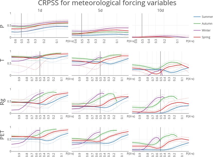
B. van Osnabrugge et al.: Contribution of PET to 10-day forecast skill                                                            1455

Figure 1. Map of the Rhine basin, Europe. Black lines delineate 148 subbasins used in the analysis of the meteorological forecast skill.
Square markers show the locations used for forecast skill analysis.

         n
                                                                                                          !
         X                                                                        n
                                                                                  X
Tm,x =         Tm,i wi,x .                                    (2)     Tγ ,x = γ         (Hi − Hx ) wi,x                             (3)
         i=1                                                                      i=1

Third, calculate the temperature lapse correction term Tγ ,x          Note that Tγ ,x is static for a fixed configuration of the mea-
as the weighted difference between the height of the grid             surement network if γ is taken to be a constant. In this study
cell Hx and the height of the considered stations Hi multi-           the configuration of the measurement network changed based
plied by the lapse rate γ .                                           on the number of reporting stations at each time step. A con-
                                                                      stant lapse rate was assumed: γ = 0.0066 (◦ C m−1 ).

www.hydrol-earth-syst-sci.net/23/1453/2019/                                         Hydrol. Earth Syst. Sci., 23, 1453–1467, 2019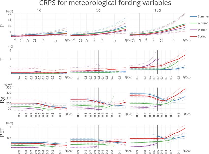
1456                                                 B. van Osnabrugge et al.: Contribution of PET to 10-day forecast skill

  The final temperature estimate for grid cell x is obtained      gridded model had the best overall results (Bowman et al.,
by adding Tγ ,x and Tm,x :                                        2017).
                                                                     A disadvantage of using satellites such as MODIS is their
Tx = Tγ ,x + Tm,x .                                        (4)    temporal coverage which is restricted to a single overpass at
                                                                  a set time each day giving one instantaneous value. This can
2.3    Downward shortwave surface radiation flux
                                                                  be resolved by assuming a sinusoidal development of PET
The availability of solar radiation measurements at the sur-      over the day (Kim and Hogue, 2008), but the limitation is
face has proven to be spatially and temporally inadequate         clear. This disadvantage is resolved by using geostationary
for many applications, with remotely sensed solar radiation       satellites. For example, Jacobs et al. (2009) used solar radia-
products having the largest potential to remedy this (Journée     tion from the NOAA GOES geostationary satellite in combi-
and Bertrand, 2010). Remotely sensed solar radiation esti-        nation with ground observations to calculate daily PET with
mates from the Land Surface Analysis Satellite Application        the Penman–Monteith equation.
Facility (LSA-SAF) were found to be in closer agreement              Here, potential evaporation is calculated from geostation-
with ground observations than reanalysis datasets such as the     ary satellite radiation estimates and ground observations of
Système d’Analyze Fournissant des Renseignements Atmo-            temperature with the method proposed by Makkink (1957),
sphériques à la Neige (SAFRAN) reanalysis (Carrer et al.,         which is applicable with remotely sensed radiation estimates
2012) and ERA-Interim (Jedrzej et al., 2014).                     (de Bruin et al., 2016). PET calculated with Makkink’s equa-
   For this study, downward shortwave radiation is resampled      tion is a reference crop evapotranspiration, which means that
and merged from the EUMETSAT Surface Incoming Solar               crop factors apply determined by the hydrological model. In
Radiation (SIS) (Mueller et al., 2009) and Downward Sur-          the setup of our hydrological model the crop factor was de-
face Shortwave Flux (DSSF) (Trigo et al., 2011) products          termined by land use. A crop factor of 1.15 is applied to the
from the Climate Monitoring Satellite Application Facility        forested areas, and 1.0 to all others.
(CM-SAF) and LSA-SAF, respectively. Gaps in the satellite            The reasons for choosing the Makkink equation are that
data are filled with the ERA5 surface solar radiation down-       (1) it only needs radiation and temperature, for which grid-
wards (ssrd) parameter from the 4d-var reanalysis (Coperni-       ded estimations are available, and that (2) the Makkink equa-
cus Climate Change Service, 2018). ERA5 was found to have         tion is used by the Royal Netherlands Meteorological Insti-
comparable mean bias with satellite-derived products for in-      tute (KNMI), so that the work presented here is compatible
land stations (Urraca et al., 2018).                              with ongoing local research (Hiemstra and Sluiter, 2011).
   In earlier research it has been shown that LSA-SAF                The potential evaporation is calculated based on air tem-
(2005–current) and CM-SAF (1983–2005) can consistently            perature T (◦ C) and downward shortwave radiation Rg
be merged into one time series (Jedrzej et al., 2014). The        (W m−2 ) for accumulation period t (s) (Hiemstra and Sluiter,
products of the different SAFs are comparable in terms of         2011):
bias and standard deviation (Ineichen et al., 2009).                                    1    tRg
                                                                  PET = 1000 · 0.65        ·     (mm),                       (5)
                                                                                      1 + ψ λρw
2.4    Makkink potential evaporation
                                                                  with ψ the psychrometric constant, λ the latent heat of water,
There are different approaches in making use of remotely          1 the slope of the saturation vapor pressure curve and ρw the
sensed data to calculate evapo(transpi)ration. One branch of      density of water calculated by
research aims to calculate actual evapotranspiration directly                             h           i
from satellite imagery (Su, 2002). Applications range from        ψ = 0.646 + 0.0006T hPa ◦ C−1 ,                           (6)
estimating the global evaporation flux (Mu et al., 2011), wa-                                 h       i
                                                                  λ = 1000(2501 − 2.38T ) J kg−1 ,                          (7)
ter resources management (Bastiaanssen et al., 2005) and
constraining model parameters for a gridded model (Im-                 6.107 · 7.5 · 273.3 7.5T     h        i
merzeel and Droogers, 2008).                                      1=                      e 273.3+T hPa ◦ C−1 ,             (8)
                                                                          (273.3 + T )2
   For operational use, PET estimates can be derived from                     h        i
satellite data only, or from a combination of satellite imagery   ρw = 1000 kg m−3 .                                        (9)
and ground measurements. Bowman et al. (2017) explored            The Makkink potential evaporation calculated for each time
the use of MODIS to provide a daily PET, both as dynamic          step is called “near real time” (PETNRT ). The potential evap-
PET (Spies et al., 2015) and PET climatology (Bowman              oration climatology (PETClim ) was calculated by averaging
et al., 2016) for a gridded and lumped version of the Sacra-      over the full time period (20 years) for each day (Fig. 2).
mento Soil Moisture Accounting (SAC-SMA) model. The
model was recalibrated for each PET input. No configuration       2.5   ECMWF reforecast
with MODIS-derived PET showed consistent improvements
across all basins in their case study. Still, it was concluded    The European Center for Medium-Range Weather Fore-
that the combination of dynamic PET in combination with a         casts (ECMWF) issues hindcasts produced with the current

Hydrol. Earth Syst. Sci., 23, 1453–1467, 2019                                  www.hydrol-earth-syst-sci.net/23/1453/2019/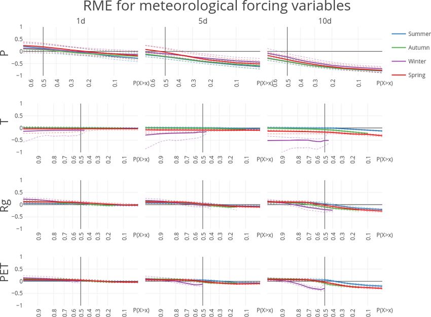
B. van Osnabrugge et al.: Contribution of PET to 10-day forecast skill 1457
Figure 2. Difference between climatology and near-real-time potential evaporation. Shown for the year 2004 for grid cell x : 200, y : 200.
model cycle for certain days for the last 20 years. The re- tion (GLUE) like procedure (Beven and Binley, 1992), us-
forecast obtained for this study was produced with model ing HYRAS precipitation as forcing data (Winsemius et al.,
cycle 43r1 (Buizza et al., 2017). The first forecast is on 2013a, b). The model is taken “as is” and is not recalibrated
10 March 1996 and the last forecast on 29 December 2015, for each PET forcing, the effect of which has been studied ex-
with reforecasts alternating every 3 or 4 days. tensively elsewhere (e.g., Bowman et al., 2017; Oudin et al.,
Forecasted Makkink potential evaporation (PETFcast ) is 2005a).
calculated based on the t2m (T ) and ssrd (Rg ) variables using
Eqs. (5)–(9). Temperature was first downscaled to the model
resolution using the standard lapse rate as used in the inter- 3 Experimental setup
polation of the temperature observations as follows:
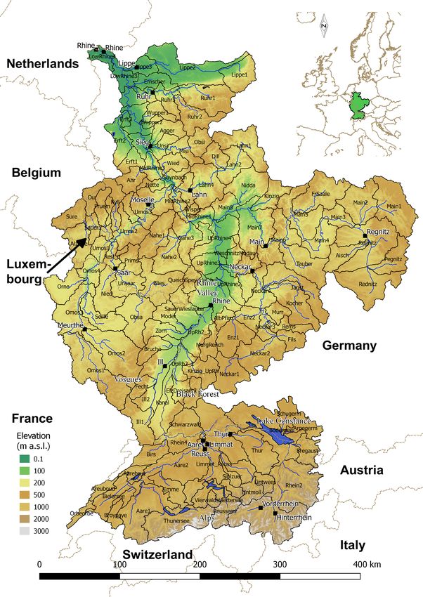
The analysis consists of a meteorological part and a hydro-
Tx = T + h − hx γ , (10) logical part (Fig. 3).
with T the temperature given by the ECMWF forecast on the 3.1 Analysis of meteorological forecast skill
ECMWF resolution, h the average height of the DEM cor-
responding to the footprint of the ECMWF grid cell, hx the In this analysis we aim to answer the following question.
height of cell x in the model, and γ the lapse rate. What is the forecast skill of temperature, radiation and po-
tential evaporation compared to precipitation?
2.6 Hydrological model For this purpose the observations and forecasts are spa-
tially averaged over 148 subbasins (Fig. 1). Time series of ob-
wflow is a modular hydrological modeling framework that al- servations and forecasts are then used to calculate the mean
lows for easy implementation and prototyping of regular grid continuous ranked probability skill score (CRPSS) for each
hydrological model concepts in python-pcraster (Schellekens basin and each season (MAM, JJA, SON, DJF).
et al., 2017). The hydrological model concept used is the The mean continuous ranked probability score (CRPS) is
HBV (Hydrologiska Byråns Vattenbalansavdelning) model an overall measure of forecast quality and is calculated by
concept (Lindström et al., 1997) applied on a grid basis. The
generated runoff is routed through the river network with a n Z∞
1X
kinematic wave approach (Schellekens et al., 2017). In the CRPS = Fy (y) − H(y ≥ x) dy, (11)
following this model is referred to as wflow_hbv. The setup n i=1
−∞
of the hydrological model is the same as used in assess-
ing the validity of the genRE precipitation dataset (van Os- in which Fy (y) is the cumulative distribution function of the
nabrugge et al., 2017). The model was parameterized through forecast variable and H(y ≥ x) the Heaviside step function
calibration with a generalized likelihood uncertainty estima- that assumes probability 1 for values greater than or equal
www.hydrol-earth-syst-sci.net/23/1453/2019/ Hydrol. Earth Syst. Sci., 23, 1453–1467, 2019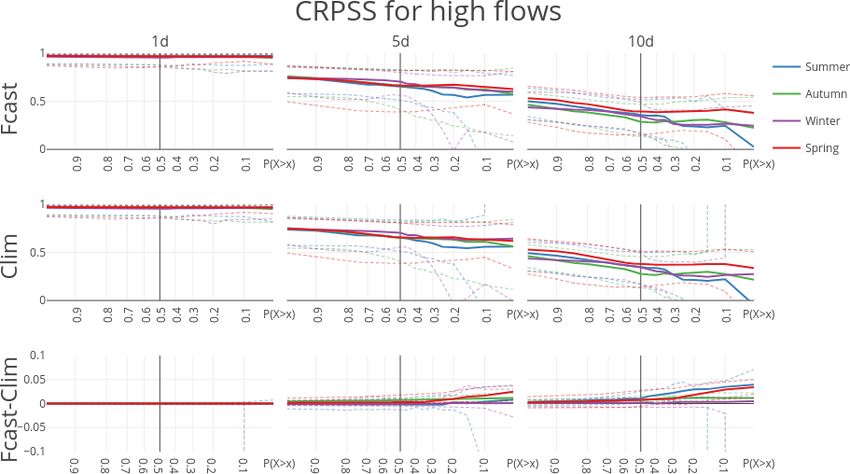
1458                                                        B. van Osnabrugge et al.: Contribution of PET to 10-day forecast skill

Figure 3. Flow chart of the model experiment. Blue boxes represent data products. Green boxes depict modeling activities. Arrows represent
the flow of data for historical runs (blue lines) and forecast runs (black). The red boxes indicate the areas for analysis of the results, each box
targeting a research subquestion.

to the observation and 0 otherwise (Brown et al., 2010). In-                  1. To what extent are initial states affected by the use of
terpretation of the mean CRPS is similar to interpretation of                    climatological versus near-real-time potential evapora-
a root mean square error. Both scores have no fixed upper                        tion?
bound, their magnitude is determined by the variable, and
lower scores are better, with 0 the perfect score.                            2. To what extent can potential evaporation forecasts con-
   The limits of the mean CRPS vary depending on the basin                       tribute to streamflow forecast skill?
and season, and it is therefore difficult to compare between                  To answer the first question, the wflow_hbv model is con-
basins and season. For this reason the CRPS is translated into              secutively forced with PETClim and PETNRT . Four states and
the continuous ranked probability skill score, which mea-                   two fluxes are exported for analysis: (1) upper soil reser-
sures the performance of a forecasting system relative to a                 voir, (2) lower soil reservoir, (3) interception storage, (4) soil
reference forecast. The reference forecast here is seasonal                 moisture store and fluxes, (5) discharge and (6) actual evap-
climatology. As such the CRPSS equals 1 for a perfect fore-                 oration. For the different states and fluxes the mean differ-
cast and 0 when the forecast ensemble does not score a better               ence (MD) is calculated for each grid cell. This is done for
CRPS than the CRPS calculated for the climatological distri-                each season to investigate seasonality of differences. The
bution.                                                                     MD is calculated as
            CRPSREF − CRPS                                                           n
CRPSS =                                                          (12)                P
                                                                                           STATENRT,i − STATECLIM,i
                    CRPSREF                                                          i=1
                                                                            MD =                                               .              (14)
Additionally, the relative mean error (RME) is calculated for                                           n
the mean of the forecasts Yi to detect relative biases in the               To answer the second question, two hindcast runs are per-
mean:                                                                       formed with PETFcast and PETClim as PET forcing, respec-
          n
          P                                                                tively. To avoid effects caused by the initial state, all forecasts
                Yi − xi                                                     start from the initial states derived from the PETNRT simula-
          i=1
RME =           n              ,                                 (13)       tion. Forecast skill scores are calculated as for the meteoro-
                P
                      xi                                                    logical variables for 20 discharge gauges and for each season.
                i=1                                                         Different from the meteorological verification exercise, the
in which Yi is the mean of the ensemble for forecast i and                  metrics are calculated for the forecasts with reference to the
xi the corresponding observation.                                           model output, and are not compared with observations. The
   The above scores are calculated with the Ensemble Veri-                  reason for this was that differences between observation and
fication System (EVS), a software package to calculate en-                  forecast stem from many different sources, including errors
semble verification metrics (Brown et al., 2010).                           in the initial state. Subsequently, a forecast that is “too wet”
                                                                            might compensate in the 10-day forecast for initial states that
3.2    Analysis of the effect of PET forecasts on                           were “too dry”. For this reason the effect of the meteorolog-
       streamflow predictions                                               ical forecast was isolated by calculating the verification met-
                                                                            rics against modeled streamflow. This also avoids issues of
In this second part of the analysis we aim to answer the fol-               perceptive bias due to the model being calibrated on another
lowing questions.                                                           PET forcing; one of the PET types might simply perform

Hydrol. Earth Syst. Sci., 23, 1453–1467, 2019                                               www.hydrol-earth-syst-sci.net/23/1453/2019/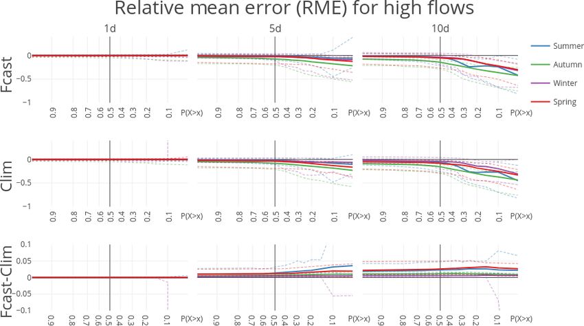
B. van Osnabrugge et al.: Contribution of PET to 10-day forecast skill                                                      1459

better because it is more like the original PET used in cali-      forecast. For temperature the 1-day forecast is close to per-
bration.                                                           fect for autumn and spring. The skill in temperature forecast
  Streamflow gauges for analysis were selected such that           is similar for spring, summer and autumn but worse during
                                                                   winter. The spread, the difference in skill between basins, is
    1. only gauges were chosen for which the model was             also largest during winter and spring. The RME shows that
       deemed behavioral as expressed by a KGE score thresh-       there is a small negative bias in the temperature forecasts.
       old of 0.5;                                                 The RME for winter is largest; however, it should be noted
                                                                   that the RME is the mean difference weighed by the mean of
    2. only one gauge was selected for each stream in the          the observations (Eq. 13). As the mean temperature in winter
       basin, except for the Rhine River itself, for which         is closer to zero, this results in larger RME. Still, also when
       two additional gauges were chosen. If multiple gauges       expressed in absolute values, the error for temperature during
       in the same stream were present, the gauge most down-       winter is larger than for other seasons (Fig. 5).
       stream was chosen. The gauge “most downstream” was             For radiation there is already quite a considerable loss in
       selected by sorting on mean yearly discharge and pick-      skill after 1 day, but then the CRPSS remains quite stable for
       ing the highest; and                                        longer forecasts, notably during spring and autumn. There is
                                                                   a larger decline in skill for summer and for extreme low radi-
    3. from the then remaining list, the largest 20 streams were
                                                                   ation values in winter. In absolute terms, the CRPS is related
       selected for analysis.
                                                                   to the magnitude of the average radiation for each season,
The streamflow locations are shown in Fig. 1 as black squares      with the smallest absolute errors for winter and the largest
including the name of the river.                                   during summer (Fig. 5). In terms of bias, we see that the
                                                                   relative mean error increases with lower P (X ≥ x) (Fig. 6,
                                                                   row 3). This indicates that low values are slightly overesti-
4     Results                                                      mated while high values are slightly underestimated, making
                                                                   the radiation forecasts slightly less extreme than the obser-
4.1    Analysis of meteorological forecast skill                   vations. This is further demonstrated in Fig. S1 in the Sup-
                                                                   plement, which plots the RME for different levels of non-
The forecast skill is assessed for all catchments and for          exceedance (P (X ≤ x)), as opposed to exceedance in Fig. 6.
each season. Seasons are Northern Hemisphere seasons                  The skill of the potential evaporation forecast is closely
spring (MAM), summer (JJA), autumn (SON), and win-                 tied to the skill in radiation forecast, both because Makkink
ter (DJF). Figure 4 shows the mean CRPSS calculated for            potential evaporation is directly proportional to radiation and
subsamples of all forecast–observation pairs for different lev-    because of the larger uncertainty in the radiation forecast.
els of exceedance, P (X ≥ x), for each variable. Simply put,       The forecast skill has the same properties as those found for
the CRPSS value at P (X ≥ x) = 0.1 is calculated for the top       the radiation forecast. A small difference is that part of the
10 % of observations and the CRPSS value at P (X ≥ x) =            forecast skill in temperature is found back in a slightly im-
0.7 is calculated for the highest 70 % of the observations.        proved forecast skill after 10 days for PET compared to radi-
P (X ≥ x) is calculated over all observations from all sea-        ation in summer.
sons. This means that for some seasons, for example tem-              Overall, there is relatively little spread in skill between
perature in winter, there is a lower limit in P (X ≥ x), be-       basins, with the 10th and 90th percentiles close to the mean
cause the highest temperatures do not occur during winter.         and following the same trajectory. The difference in skill be-
On the other hand, the response of the CRPSS curve is flat for     tween the different seasons is larger than the spread between
high P (X ≥ x) for temperature during summer, as all sum-          basins, especially for the variables temperature, radiation and
mer temperatures fall in the highest 60 % of temperatures of       potential evaporation. This difference in skill between sea-
the whole year. The same is shown for the CRPS, Fig. 5, and        sons is partly misleading. For example, the forecast skill for
the RME, Fig. 6.                                                   radiation in winter (Fig. 4, purple line) appears to be an out-
   There is no skill in the ECMWF forecast beyond 10 days          lier. However, the whole range of occurrences of extreme
for daily precipitation. This is consistent with the 9-day lead    high and low radiative forcing is compressed in a limited part
time in streamflow forecasts found by Renner et al. (2009).        of P (X ≥ x). Although the forecast over the whole range of
The skill is best in winter and worst in summer, which is          winter radiative forcing is lower than that for the other sea-
expected based on the dominating meteorological processes          sons, the top 10 % of winter radiative forcings are actually
(frontal systems in winter and convective events in summer).       among the best predicted.
The total amount of precipitation is underestimated after a           Likewise, high temperatures receive higher skill scores
1-day lead time (Fig. 6).                                          than low season temperatures. This is even more distinct in
   There is more skill in the forecast for the variables tem-      the radiation forecasts. This does, however, not mean that the
perature and incoming shortwave radiation. Likewise, there         forecasts of such rare events are more accurate: both RME
is considerable skill remaining in the potential evaporation       (Fig. 6) and CRPS (Fig. 5) are larger for high extremes,

www.hydrol-earth-syst-sci.net/23/1453/2019/                                     Hydrol. Earth Syst. Sci., 23, 1453–1467, 2019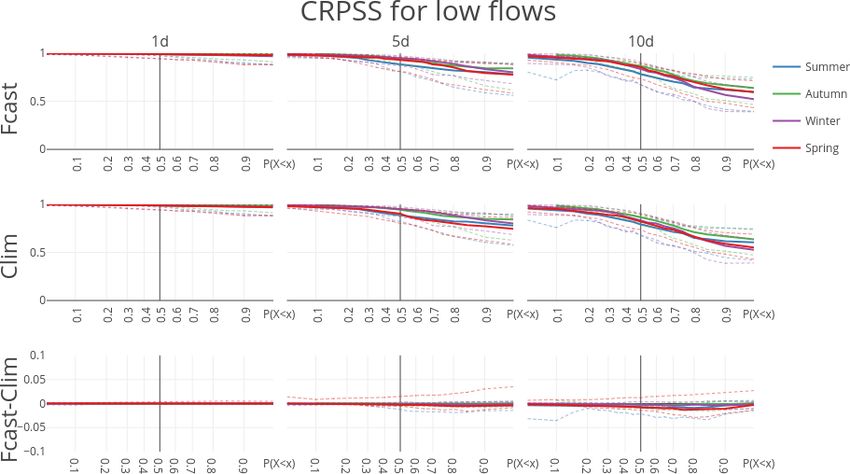
1460                                                   B. van Osnabrugge et al.: Contribution of PET to 10-day forecast skill

Figure 4. Continuous ranked probability skill score (CRPSS) for the four forcing variables benchmarked against sample climatology for the
148 HBV subbasins. CRPSSs are aggregated into mean (solid), 10th and 90th percentiles (dashed). Note that the CRPSS at P (X ≥ x) = 0.1
or 0.7 is calculated over, respectively, the 10 % and 70 % highest observation–forecast pairs, conditioned on the observations.

meaning larger errors for those forecasts. Still, taking into ac-      from the interception store. The latter is sometimes taken into
count the rarity of the event by calculating the CRPSS, which          account in hydrological models by adding a potential evapo-
is the skill of the forecast relative to the skill of a random         ration reduction function dependent on the intensity of pre-
draw from the climatology, temperature, radiation and poten-           cipitation to correct the PET climatology. For example, the
tial evaporation forecasts are found to add most information           HBV model has this option (Schellekens et al., 2017).
for extreme high values, even though the error of those fore-             The lower evaporation with dynamic PET forcing cas-
casts is larger than for more “average” values (values with a          cades through the different model storages, accumulating in
higher probability of occurrence).                                     a mostly wetter lower zone (LZ) storage under dynamic forc-
                                                                       ing. Finally, the lower evaporation results in higher discharge
4.2    Influence of dynamic PET on initial states                      throughout the Rhine basin (see Figs. S2–S7). Exceptions are
                                                                       the high Rhine during spring and to a lesser extent during au-
                                                                       tumn, and several areas during winter when there is very lit-
Dynamic potential evaporation leads to lower actual evapora-
                                                                       tle effect overall. The wetter conditions also result in higher
tion (AET). The difference is largest for summer and spring
                                                                       peak discharges. As these higher discharges are a result of
(Fig. 7). Part of this lower evaporation is from a reduction
                                                                       the temporal dynamics of the potential evaporation input, we
in interception as the interception storage is more filled on
                                                                       expect to find a similar effect on forecasted discharges. As
average under dynamical forcing. This can be explained by
                                                                       will be shown later (Fig. 9), this is indeed the case, albeit
the correlation between precipitation events and low poten-
                                                                       very limited.
tial evaporation. On rainy days the dynamic potential evapo-
ration is generally lower, which decreases the amount of in-
terception evaporation. Under climatological forcing the en-
ergy available is not reduced, and thus more water evaporates

Hydrol. Earth Syst. Sci., 23, 1453–1467, 2019                                        www.hydrol-earth-syst-sci.net/23/1453/2019/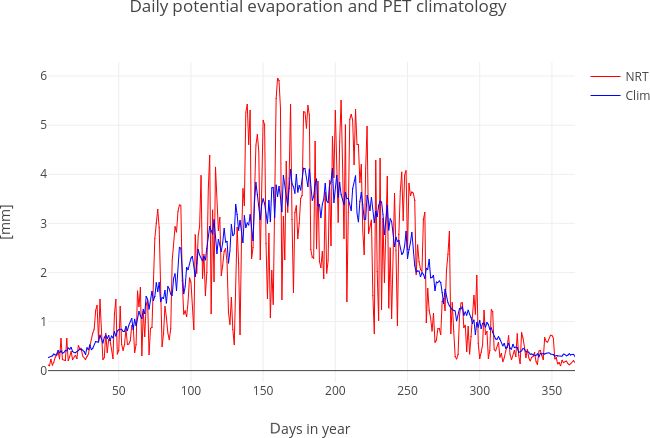
B. van Osnabrugge et al.: Contribution of PET to 10-day forecast skill                                                                    1461

Figure 5. Continuous ranked probability score (CRPS) for the four forcing variables for the 148 HBV subbasins for the whole year. CRPS is
aggregated into mean (solid), 10th and 90th percentiles (dashed). Note that the CRPS at P (X ≥ x) = 0.1 or 0.7 is calculated over, respectively,
the 10 % and 70 % highest observation–forecast pairs, conditioned on the observations.

4.3   Influence of PET forecast on streamflow forecast                    mer, as shown by the largest decrease in CRPSS for the 10-
                                                                          day forecast in summer compared to the other seasons. The
                                                                          CRPSS especially “dips” for the most extreme discharges,
The CRPSS for streamflow forecast is hardly influenced by
                                                                          which is not as strong for spring and autumn, and especially
potential evaporation forcing type. At first sight, the skill
                                                                          compared to the flat response of the CRPSS for the highest
scores obtained with dynamic or climatological PET are
                                                                          30 % of discharges in winter.
identical. Small differences only become visible when tak-
                                                                             In terms of the effect of potential evaporation climatol-
ing a close-up of the differences by subtracting one from the
                                                                          ogy versus forecasted potential evaporation, the influence is
other (Fig. 8). However, the small difference in skill grows
                                                                          largest (but still quite small) for summer and spring. This is
with lead time. The influence of PET forcing type becomes
                                                                          tied to the potential evaporation being of larger magnitude;
more intuitive when looking at the RME. An increasing drift
                                                                          there is hardly a response for winter, where there is the low-
with lead time between PET forcing types is visible (Fig. 9).
                                                                          est potential evaporation.
Interestingly, this drift in RME is almost uniform over all
                                                                             The influence of PET forecasts on low flow prediction is
subsets of predicted discharge. The drift is positive, which
                                                                          further examined by calculating the scores for different levels
means that forecasted PET leads to slightly higher forecasted
                                                                          of non-exceedance P (X ≤ x), instead of exceedance, so that
discharges, as expected based on the results of the influence
                                                                          the score value at P (X ≤ x) = 0.1 is calculated for the 10 %
of variable PET on the initial states.
                                                                          smallest observations and the score value at P (X ≤ x) = 0.7
   Analyzed for each season separately, there is a little more
                                                                          is calculated for the lowest 70 % of the observations. Not
to discover about the role of potential evaporation forecasts
                                                                          only has the choice of PET forcing for the forecast hardly
and the sensitivity of forecast skill to the meteorological fore-
                                                                          any effect on the forecasted streamflow (Fig. 10, bottom
cast in general. The contribution of the meteorological fore-
                                                                          row), but the forecast skill of low discharge is also affected
cast to streamflow forecast uncertainty is largest for sum-

www.hydrol-earth-syst-sci.net/23/1453/2019/                                              Hydrol. Earth Syst. Sci., 23, 1453–1467, 2019
1462 B. van Osnabrugge et al.: Contribution of PET to 10-day forecast skill
Figure 6. Relative mean error (RME) for the four forcing variables for the 148 HBV subbasins for the whole year. RME is aggregated into
mean (solid), 10th and 90th percentiles (dashed). Note that the CRPSS at P (X ≥ x) = 0.1 or 0.7 is calculated over, respectively, the 10 %
and 70 % highest observation–forecast pairs, conditioned on the observations.
only slightly by the skill of the meteorological forecast in days. Variable PET forcing resulted in lower evaporation and
general. The meteorological forecast skill declines with lead in wetter initial states and higher modeled discharges.
time (e.g., Fig. 4), but the forecast skill of low percentile dis- The main result of this study is that potential evapora-
charge remains almost perfect (very close to 1) compared to tion forecasts improved streamflow forecasts only slightly.
the model under perfect forcing. This confirms earlier results that the influence of random er-
rors on estimated streamflow was generally not measurable
when comparing model runs directly, needing a 20% system-
5 Conclusions atic bias in PET to influence model outcomes significantly
(Parmele, 1972). Likewise, Fowler (2002) concluded that cli-
This paper presented a simple and straightforward inves-
matological PET estimates produced a soil water regime very
tigation with an operational forecasting practice perspec-
similar to that derived with actual daily PET values, includ-
tive. First, observation data were preprocessed for use in the
ing extreme periods, for a site in Auckland, New Zealand.
gridded wflow_hbv model. Second, the wflow_hbv model
There is a wider discussion on evaporation modeling in
was subjected to dynamical and climatological PET forcing.
hydrological models (Andréassian et al., 2004; Oudin et al.,
Three aspects were analyzed: (1) the skill in meteorological
2005a; Oudin et al., 2005b) to which the results here might
forecast, (2) the effect of PET forcing on initial states and
add a new perspective: that of evaporation as a process rele-
(3) the effect of PET forcing on forecast skill.
vant for medium-term forecasts. This is directly also a limi-
Nine to 10 days is the upper limit on forecast lead time
tation of this research; only the influence on forecasts up to
for daily precipitation for the ECMWF forecast in the Rhine
10 days was investigated. The influence on seasonal forecast-
basin, with only very little skill remaining compared to cli-
ing might be more substantial, considering that the modeling
matology. There is considerable skill in daily temperature,
of evaporation strongly influences the partitioning between
radiation and potential evaporation forecasts, also after 10
Hydrol. Earth Syst. Sci., 23, 1453–1467, 2019 www.hydrol-earth-syst-sci.net/23/1453/2019/B. van Osnabrugge et al.: Contribution of PET to 10-day forecast skill 1463 Figure 7. Seasonal mean difference in calculated actual evaporation (AET) for each season. Actual evaporation includes evaporation from interception. runoff and evaporation in the longer-term water balance (Bai Indeed, it is a recurring hypothesis that potential evaporation et al., 2016). forecasts should aid especially in making low flow predic- Further limitations are that only one model was tions. The uniform response of several skill scores for differ- tested (wflow_hbv) and for one climate zone (moderate tem- ent subsets of observed discharge does not support this idea; perate). The model was calibrated originally on a different there is no special gain for low flows. PET climatology than studied here and was not recalibrated. Instead, from our model results it follows that the cor- The latter is not seen as a limitation. Deliberately not re- rect prediction of a drought is firstly dependent on a correct calibrating the model enabled us to focus on the changes in forecast of no rain. Low flow recession is subsequently de- modeled processes instead of comparably vague assessments termined, in the absence of further feedback mechanisms, based on model performance expressed in efficiencies, with solely by the storage–discharge relationship of, in this case, the effects brought forward by the PET forcing hidden some- the lower zone representing the saturated zone as well as the where in the parameter space. routing of surface water. In the analysis, forecasting metrics were calculated over The follow-up question then is the following. Is this true in subsets of observation–forecast pairs conditioned on the ob- reality, or is this a model deficiency? Should we rethink hy- servations. Alternatively, the subsets could have been condi- drological modeling to incorporate more feedbacks on evap- tioned on the mean of the forecasts. This would present more oration? Certainly there are models with more complex rep- intuitive information for a forecaster at the time of a forecast resentation of evaporative processes. These are valid and im- when the observation is by definition not yet known (Lerch portant questions, especially in the light of hydrologic re- et al., 2015). sponse to change in climate drivers. However, from the re- The idea to look at potential evaporation forecast was insti- sults presented here, it should not be expected that a better gated as part of a program to improve forecasts of low flows. understanding of evaporative processes and feedbacks will www.hydrol-earth-syst-sci.net/23/1453/2019/ Hydrol. Earth Syst. Sci., 23, 1453–1467, 2019
1464                                                     B. van Osnabrugge et al.: Contribution of PET to 10-day forecast skill

Figure 8. CRPSS for forecast runs (forecasted PET, climatological PET) and their difference benchmarked against model output for the
20 largest sub-catchments in the Rhine basin. CRPSSs are aggregated into mean (solid), 10th and 90th percentiles (dashed). Note that the
CRPSS at P (X ≥ x) = 0.1 or 0.7 is calculated over, respectively, the 10 % and 70 % highest observation–forecast pairs, conditioned on the
observations.

Figure 9. RME for forecast runs (forecasted PET, climatological PET) and their difference for the 20 largest streams in the Rhine basin. RME
scores are aggregated into mean (solid), 10th and 90th percentiles (dashed). Note that the CRPSS at P (X ≥ x) = 0.1 or 0.7 is calculated
over, respectively, the 10 % and 70 % highest observation–forecast pairs, conditioned on the observations.

Hydrol. Earth Syst. Sci., 23, 1453–1467, 2019                                          www.hydrol-earth-syst-sci.net/23/1453/2019/
B. van Osnabrugge et al.: Contribution of PET to 10-day forecast skill                                                                  1465

Figure 10. CRPSS for forecast runs (forecasted PET, climatological PET) and their difference benchmarked against model output for the
20 largest streams in the Rhine basin. CRPSSs are aggregated into mean (solid), 10th and 90th percentiles (dashed). Note that the CRPSS at
P (X ≤ x) = 0.1 or 0.7 is calculated over, respectively, the 10 % and 70 % lowest observation–forecast pairs, conditioned on the observations.

result directly in a significant increase in 10-day predictive           the Dutch Ministry of Infrastructure and the Environment. Part of
skill for streamflow.                                                    the work was conducted as an in-kind contribution to Netherlands
                                                                         Organisation for Scientific Reasearch project “SWM-EVAP: Smart
                                                                         Water Management in a complex environment: improving the moni-
Data availability. Gridded precipitation, temperature, radiation         toring and forecasting of surface evaporation” (ALWTW.2016.049).
and potential evaporation used in this study are available through the   Meteorological data for this research have been gratefully received
4TU data center; see van Osnabrugge (2017) and van Osnabrugge            from the Deutscher Wetterdienst Climate Data Center; KNMI
(2018).                                                                  Data Centrum; Météo France; Federal Office of Meteorology
                                                                         and Climatology MeteoSwiss; Administration de la gestion de
                                                                         l’eau du Grand-Duché de Luxembourg; and Service Publique
                                                                         de Wallonie Département des Etudes et de l’Appui à la Gestion.
Supplement. The supplement related to this article is available
                                                                         Discharge data have been gratefully received from SCHAPI
online at: https://doi.org/10.5194/hess-23-1453-2019-supplement.
                                                                         (Service Central d’Hydrométéorologie et d’Appui àla Prévision
                                                                         des Inondations) through Banque HYDRO; Bundesamt für Umwelt
                                                                         BAFU; Bundesanstalt für Gewässerkunde (BfG); Administration
Author contributions. BvO prepared the data, performed the anal-         de la gestion de l’eau du Grand-Duché de Luxembourg; Bavar-
yses and wrote the article. RU contributed to improving the article      ian Environment Agency, https://www.lfu.bayern.de/index.htm;
and experimental setup. AW supplied part of the scripts used in the      Landesanstalt für Umwelt, Messungen und Naturschutz Baden-
analysis and contributed in preprocessing steps of the forecasts as      Württemberg, LUBW; Landesamtes für Umwelt, Wasserwirtschaft
well as contributing to the design of the model experiments and final    und Gewerbeaufsicht Rheinland-Pfalz; Landesamt für Umwelt-
article text.                                                            und Arbeitsschutz Saarland; and Landesamt für Natur, Umwelt und
                                                                         Verbraucherschutz Nordrhein-Westfalen. We thank David Lavers
                                                                         from ECMWF for providing access to the reforecast dataset.
Competing interests. The authors declare that they have no conflict
of interest.                                                             Edited by: Alexander Gelfan
                                                                         Reviewed by: two anonymous referees

Acknowledgements. This work is partly supported by the IM-
PREX project funded by the European Commission under the
Horizon 2020 framework program (grant 641811) and partly by

www.hydrol-earth-syst-sci.net/23/1453/2019/                                             Hydrol. Earth Syst. Sci., 23, 1453–1467, 2019
1466 B. van Osnabrugge et al.: Contribution of PET to 10-day forecast skill
References Remote Sensing Application, J. Hydrometeorol., 17, 1373–1382,
https://doi.org/10.1175/JHM-D-15-0006.1, 2016.
Farr, T. G., Rosen, P. A., Caro, E., Crippen, R., Duren, R.,
Andréassian, V., Perrin, C., and Michel, C.: Impact of imper- Hensley, S., Kobrick, M., Paller, M., Rodriguez, E., Roth,
fect potential evapotranspiration knowledge on the efficiency L., Seal, D., Shaffer, S., Shimada, J., Umland, J., Werner,
and parameters of watershed models, J. Hydrol., 286, 19–35, M., Oskin, M., Burbank, D., and Alsdorf, D. E.: The shut-
https://doi.org/10.1016/j.jhydrol.2003.09.030, 2004. tle radar topography mission, Rev. Geophys., 45, RG2004,
Bai, P., Liu, X., Yang, T., Li, F., Liang, K., Hu, S., Liu, C., Bai, P., https://doi.org/10.1029/2005RG000183, 2007.
Liu, X., Yang, T., Li, F., Liang, K., Hu, S., and Liu, C.: Assess- Fowler, A.: Assessment of the validity of using mean potential
ment of the Influences of Different Potential Evapotranspiration evaporation in computations of the long-term soil water bal-
Inputs on the Performance of Monthly Hydrological Models un- ance, J. Hydrol., 256, 248–263, https://doi.org/10.1016/S0022-
der Different Climatic Conditions, J. Hydrometeorol., 17, 2259– 1694(01)00542-X, 2002.
2274, https://doi.org/10.1175/JHM-D-15-0202.1, 2016. Hiemstra, P. and Sluiter, R.: Interpolation of Makkink evapo-
Bastiaanssen, W. G. M., Noordman, E. J. M., Pelgrum, H., Davids, ration in the Netherlands, Tech. rep., KNMI, De Bilt, avail-
G., Thoreson, B. P., and Allen, R. G.: SEBAL Model with Re- able at: http://bibliotheek.knmi.nl/knmipubTR/TR327.pdf (last
motely Sensed Data to Improve Water-Resources Management access: 5 March 2018), 2011.
under Actual Field Conditions, J. Irrig. Drain. Eng., 131, 85– Immerzeel, W. W. and Droogers, P.: Calibration of
93, https://doi.org/10.1061/(ASCE)0733-9437(2005)131:1(85), a distributed hydrological model based on satel-
2005. lite evapotranspiration, J. Hydrol., 349, 411–424,
Beven, K. and Binley, A.: The future of distributed models: Model https://doi.org/10.1016/j.jhydrol.2007.11.017, 2008.
calibration and uncertainty prediction, Hydrol. Process., 6, 279– Ineichen, P., Barroso, C. S., Geiger, B., Hollmann, R., Mar-
298, https://doi.org/10.1002/hyp.3360060305, 1992. souin, A., and Mueller, R.: Satellite Application Facilities ir-
Bowman, A. L., Franz, K. J., Hogue, T. S., and Kinoshita, A. M.: radiance products: Hourly time step comparison and vali-
MODIS-Based Potential Evapotranspiration Demand Curves for dation over Europe, Int. J. Remote Sens., 30, 5549–5571,
the Sacramento Soil Moisture Accounting Model, J. Hydrol. https://doi.org/10.1080/01431160802680560, 2009.
Eng., 21, 04015055, https://doi.org/10.1061/(ASCE)HE.1943- Jacobs, J. M., Lowry, B., Choi, M., and Bolster, C. H.:
5584.0001261, 2016. GOES Solar Radiation for Evapotranspiration Estimation
Bowman, A. L., Franz, K. J., and Hogue, T. S.: Case Studies of a and Streamflow Prediction, J. Hydrol. Eng., 14, 293–300,
MODIS-Based Potential Evapotranspiration Input to the Sacra- https://doi.org/10.1061/(ASCE)1084-0699(2009)14:3(293),
mento Soil Moisture Accounting Model, J. Hydrometeorol., 18, 2009.
151–158, https://doi.org/10.1175/JHM-D-16-0214.1, 2017. Jedrzej, J., Bojanowski, S., Vrieling, A., and Skidmore, A. K.: A
Brown, J. D., Demargne, J., Seo, D. J., and Liu, Y.: The Ensem- comparison of data sources for creating a long-term time series of
ble Verification System (EVS): A software tool for verifying daily gridded solar radiation for Europe, Solar Energy, 99, 152–
ensemble forecasts of hydrometeorological and hydrologic vari- 171, https://doi.org/10.1016/j.solener.2013.11.007, 2014.
ables at discrete locations, Environ. Model. Softw., 25, 854–872, Journée, M. and Bertrand, C.: Improving the spatio-temporal dis-
https://doi.org/10.1016/j.envsoft.2010.01.009, 2010. tribution of surface solar radiation data by merging ground and
Buizza, R., Bidlot, J.-R., Janousek, M., Keeley, S., Mogensen, K., satellite measurements, Remote Sens. Environ., 114, 2692–2704,
and Richardson, D.: New IFS cycle brings sea-ice coupling and https://doi.org/10.1016/j.rse.2010.06.010, 2010.
higher ocean resolution, ECMWF Newsletter No. 150, 14–17, Kim, J. and Hogue, T. S.: Evaluation of a MODIS-Based Potential
https://doi.org/10.21957/xbov3ybily, 2017. Evapotranspiration Product at the Point Scale, J. Hydrometeorol.,
Carrer, D., Lafont, S., Roujean, J.-L., Calvet, J.-C., Meurey, C., 9, 444–460, https://doi.org/10.1175/2007JHM902.1, 2008.
Le Moigne, P., and Trigo, I. F.: Incoming Solar and Infrared Ra- Lerch, S., Thorarinsdottir, T. L., Ravazzolo, F., and Gneiting, T.:
diation Derived from METEOSAT: Impact on the Modeled Land Forecaster’s Dilemma: Extreme Events and Forecast Evaluation,
Water and Energy Budget over France, J. Hydrometeorol., 13, Statist. Sci., 32, 106–127, https://doi.org/10.1214/16-STS588,
504–520, https://doi.org/10.1175/JHM-D-11-059.1, 2012. 2015.
Cloke, H. and Pappenberger, F.: Ensemble flood Lindström, G., Johansson, B., Persson, M., Gardelin, M., and
forecasting: A review, J. Hydrol., 375, 613–626, Bergström, S.: Development and test of the distributed
https://doi.org/10.1016/j.jhydrol.2009.06.005, 2009. HBV-96 hydrological model, J. Hydrol., 201, 272–288,
Copernicus Climate Change Service (C3S): ERA5: Fifth generation https://doi.org/10.1016/S0022-1694(97)00041-3, 1997.
of ECMWF atmospheric reanalyses of the global climate, Coper- Makkink, G. F.: Ekzameno de la formulo de Penman, Neth. J. Agri.
nicus Climate Change Service Climate Data Store (CDS), avail- Sci., 5, 290–305, 1957.
able at: https://cds.climate.copernicus.eu/cdsapp#!/home, last ac- Mu, Q., Zhao, M., and Running, S. W.: Improvements
cess: 1 July 2018. to a MODIS global terrestrial evapotranspiration al-
Cuo, L., Pagano, T. C., and Wang, Q. J.: A Review of Quantita- gorithm, Remote Sens. Environ., 115, 1781–1800,
tive Precipitation Forecasts and Their Use in Short- to Medium- https://doi.org/10.1016/j.rse.2011.02.019, 2011.
Range Streamflow Forecasting, J. Hydrometeorol., 12, 713–728, Mueller, R., Matsoukas, C., Gratzki, A., Behr, H., and Hollmann,
https://doi.org/10.1175/2011JHM1347.1, 2011. R.: The CM-SAF operational scheme for the satellite based re-
de Bruin, H. A. R., Trigo, I. F., Bosveld, F. C., and Meirink, J. F.: A trieval of solar surface irradiance – A LUT based eigenvec-
Thermodynamically Based Model for Actual Evapotranspiration
of an Extensive Grass Field Close to FAO Reference, Suitable for
Hydrol. Earth Syst. Sci., 23, 1453–1467, 2019 www.hydrol-earth-syst-sci.net/23/1453/2019/B. van Osnabrugge et al.: Contribution of PET to 10-day forecast skill 1467 tor hybrid approach, Remote Sens. Environ., 113, 1012–1024, Trigo, I. F., Dacamara, C. C., Viterbo, P., Roujean, J.-L., Ole- https://doi.org/10.1016/J.RSE.2009.01.012, 2009. sen, F., Barroso, C., Camacho-de Coca, F., Carrer, D., Fre- Oudin, L., Hervieu, F., Michel, C., Perrin, C., Andréassian, V., itas, S. C., García-Haro, J., Geiger, B., Gellens-Meulenberghs, Anctil, F., and Loumagne, C.: Which potential evapotranspi- F., Ghilain, N., Meliá, J., Pessanha, L., Siljamo, N., and ration input for a lumped rainfall-runoff model? Part 2 – Arboleda, A.: The Satellite Application Facility for Land Towards a simple and efficient potential evapotranspiration Surface Analysis, Int. J. Remote Sens., 32, 2725–2744, model for rainfall-runoff modelling, J. Hydrol., 303, 290–306, https://doi.org/10.1080/01431161003743199, 2011. https://doi.org/10.1016/j.jhydrol.2004.08.026, 2005a. Urraca, R., Huld, T., Gracia-Amillo, A., Martinez-de Pison, F. J., Oudin, L., Michel, C., and Anctil, F.: Which potential evapo- Kaspar, F., and Sanz-Garcia, A.: Evaluation of global horizontal transpiration input for a lumped rainfall-runoff model? Part 1 irradiance estimates from ERA5 and COSMO-REA6 reanalyses – Can rainfall-runoff models effectively handle detailed po- using ground and satellite-based data, Solar Energy, 164, 339– tential evapotranspiration inputs?, J. Hydrol., 303, 275–289, 354, https://doi.org/10.1016/j.solener.2018.02.059, 2018. https://doi.org/10.1016/j.jhydrol.2004.08.025, 2005b. van den Hurk, B. J., Bouwer, L. M., Buontempo, C., Döscher, R., Pappenberger, F., Beven, K. J., Hunter, N. M., Bates, P. D., Ercin, E., Hananel, C., Hunink, J. E., Kjellström, E., Klein, B., Gouweleeuw, B. T., Thielen, J., and de Roo, A. P. J.: Cas- Manez, M., Pappenberger, F., Pouget, L., Ramos, M.-H., Ward, cading model uncertainty from medium range weather fore- P. J., Weerts, A. H., and Wijngaard, J. B.: Improving predic- casts (10 days) through a rainfall-runoff model to flood in- tions and management of hydrological extremes through cli- undation predictions within the European Flood Forecast- mate services: http://www.imprex.eu/, Climate Services, 1, 6–11, ing System (EFFS), Hydrol. Earth Syst. Sci., 9, 381–393, https://doi.org/10.1016/j.cliser.2016.01.001, 2016. https://doi.org/10.5194/hess-9-381-2005, 2005. van Osnabrugge, B.: Gridded precipitation dataset for the Rhine Parmele, L. H.: Errors in output of hydrologic models due to errors basin made with the genRE interpolation method, 4TU. Centre in input potential evapotranspiration, Water Resour. Res., 8, 348– for Research Data, https://doi.org/10.4121/uuid:c875b385-ef6d- 359, https://doi.org/10.1029/WR008i002p00348, 1972. 45a5-a6d3-d5fe5e3f525d, 2017. Photiadou, C. S., Weerts, A. H., and van den Hurk, B. J. J. M.: Eval- van Osnabrugge, B.: Gridded Hourly Temperature, Radiation uation of two precipitation data sets for the Rhine River using and Makkink Potential Evaporation forcing for hydrolog- streamflow simulations, Hydrol. Earth Syst. Sci., 15, 3355–3366, ical modelling in the Rhine basin, Wageningen Univer- https://doi.org/10.5194/hess-15-3355-2011, 2011. sity & Research, Dataset, https://doi.org/10.4121/uuid:e036030f- Rauthe, M., Steiner, H., Riediger, U., Mazurkiewicz, A., and c73b-4e7b-9bd4-eebc899b5a13, 2018. Gratzki, A.: A Central European precipitation climatology – van Osnabrugge, B., Weerts, A. H., and Uijlenhoet, R.: Part I: Generation and validation of a high-resolution grid- genRE: A Method to Extend Gridded Precipitation Cli- ded daily data set (HYRAS), Meteorol. Z., 22, 235–256, matology Data Sets in Near Real-Time for Hydrological https://doi.org/10.1127/0941-2948/2013/0436, 2013. Forecasting Purposes, Water Resour. Res., 53, 9284–9303, Reggiani, P., Renner, M., Weerts, A. H., and van Gelder, P. https://doi.org/10.1002/2017WR021201, 2017. A. H. J. M.: Uncertainty assessment via Bayesian revision Verkade, J., Brown, J., Reggiani, P., and Weerts, A.: Post- of ensemble streamflow predictions in the operational river processing ECMWF precipitation and temperature en- Rhine forecasting system, Water Resour. Res., 45, W02428, semble reforecasts for operational hydrologic forecast- https://doi.org/10.1029/2007WR006758, 2009. ing at various spatial scales, J. Hydrol., 501, 73–91, Renner, M., Werner, M. G. F., Rademacher, S., and https://doi.org/10.1016/j.jhydrol.2013.07.039, 2013. Sprokkereef, E.: Verification of ensemble flow fore- Winsemius, H. M., van Verseveld, W., Weerts, A. H., and Hegnauer, casts for the River Rhine, J. Hydrol., 376, 463–475, M.: Generalised Likelihood Uncertainty Estimation for the daily https://doi.org/10.1016/j.jhydrol.2009.07.059, 2009. HBV model in the Rhine Basin, Part B: Switzerland, Tech. rep., Schellekens, J., van Verseveld, W., de Boer-Euser, T., Win- Deltares, Delft, 2013a. semius, H., Thiange, C., Bouaziz, L., Tollenaar, D., de Vries, Winsemius, H. M., van Verseveld, W., Weerts, A. H., and Hegnauer, S., and Weerts, A.: Openstreams wflow documentation, avail- M.: Generalised Likelihood Uncertainty Estimation for the daily able at: http://wflow.readthedocs.io/en/2017.01/ (last access: HBV model in the Rhine Basin, Part A: Germany, Tech. rep., 1 March 2018), 2017. Deltares, Delft, 2013b. Spies, R. R., Franz, K. J., Hogue, T. S., and Bowman, A. Xu, C.-Y. and Singh, V. P.: Cross Comparison of Empirical L.: Distributed Hydrologic Modeling Using Satellite-Derived Equations for Calculating Potential Evapotranspiration with Potential Evapotranspiration, J. Hydrometeorol., 16, 129–146, Data from Switzerland, Water Resour. Manage., 16, 197–219, https://doi.org/10.1175/JHM-D-14-0047.1, 2015. https://doi.org/10.1023/A:1020282515975, 2002. Su, Z.: The Surface Energy Balance System (SEBS) for estima- Xystrakis, F. and Matzarakis, A.: Evaluation of 13 Empirical Ref- tion of turbulent heat fluxes, Hydrol. Earth Syst. Sci., 6, 85–100, erence Potential Evapotranspiration Equations on the Island of https://doi.org/10.5194/hess-6-85-2002, 2002. Crete in Southern Greece, J. Irrig. Drain. Eng., 137, 211–222, Terink, W., Hurkmans, R. T. W. L., Torfs, P. J. J. F., and Ui- https://doi.org/10.1061/(ASCE)IR.1943-4774.0000283, 2011. jlenhoet, R.: Evaluation of a bias correction method applied to downscaled precipitation and temperature reanalysis data for the Rhine basin, Hydrol. Earth Syst. Sci., 14, 687–703, https://doi.org/10.5194/hess-14-687-2010, 2010. www.hydrol-earth-syst-sci.net/23/1453/2019/ Hydrol. Earth Syst. Sci., 23, 1453–1467, 2019
You can also read