New methods to improve the vertical extrapolation of near-surface offshore wind speeds
←
→
Page content transcription
If your browser does not render page correctly, please read the page content below
Wind Energ. Sci., 6, 935–948, 2021
https://doi.org/10.5194/wes-6-935-2021
© Author(s) 2021. This work is distributed under
the Creative Commons Attribution 4.0 License.

              New methods to improve the vertical extrapolation
                   of near-surface offshore wind speeds
                               Mike Optis, Nicola Bodini, Mithu Debnath, and Paula Doubrawa
                                  National Renewable Energy Laboratory, Golden, Colorado, USA
                                       Correspondence: Mike Optis (mike.optis@nrel.gov)

                                    Received: 22 January 2021 – Discussion started: 27 January 2021
                              Revised: 23 March 2021 – Accepted: 15 April 2021 – Published: 16 June 2021

        Abstract. Accurate characterization of the offshore wind resource has been hindered by a sparsity of wind speed
        observations that span offshore wind turbine rotor-swept heights. Although public availability of floating lidar
        data is increasing, most offshore wind speed observations continue to come from buoy-based and satellite-based
        near-surface measurements. The aim of this study is to develop and validate novel vertical extrapolation methods
        that can accurately estimate wind speed time series across rotor-swept heights using these near-surface measure-
        ments. We contrast the conventional logarithmic profile against three novel approaches: a logarithmic profile
        with a long-term stability correction, a single-column model, and a machine-learning model. These models are
        developed and validated using 1 year of observations from two floating lidars deployed in US Atlantic offshore
        wind energy areas. We find that the machine-learning model significantly outperforms all other models across all
        stability regimes, seasons, and times of day. Machine-learning model performance is considerably improved by
        including the air–sea temperature difference, which provides some accounting for offshore atmospheric stability.
        Finally, we find no degradation in machine-learning model performance when tested 83 km from its training
        location, suggesting promising future applications in extrapolating 10 m wind speeds from spatially resolved
        satellite-based wind atlases.

Copyright statement. This work was authored by the National            nical and economic analyses, ranging from grid integration
Renewable Energy Laboratory, operated by Alliance for Sustain-         (Mahoney et al., 2012), life-cycle cost analyses (Jong et al.,
able Energy, LLC, for the US Department of Energy (DOE) un-            2017), and capacity expansion studies (Hasager et al., 2015).
der contract no. DE-AC36-08GO28308. The views expressed in the            Accurate characterization of rotor-swept offshore wind
article do not necessarily represent the views of the DOE or the       speeds has been hindered by the sparsity of observations at
US Government. The US Government retains and the publisher, by
                                                                       rotor-swept heights, especially in the US offshore wind ar-
accepting the article for publication, acknowledges that the US Gov-
                                                                       eas. Offshore meteorological towers are generally too ex-
ernment retains a nonexclusive, paid-up, irrevocable, worldwide li-
cense to publish or reproduce the published form of this work, or      pensive to install, especially up to 250–300 m, i.e., the ex-
allow others to do so, for US Government purposes.                     pected upper rotor-swept heights of US offshore wind tur-
                                                                       bines. Buoy-mounted floating lidar, however, are emerging as
                                                                       a game-changing technology, especially in the United States,
1   Introduction                                                       providing accurate wind speed and direction measurements
                                                                       up to approximately 250 m (Carbon Trust, 2018); however,
The accurate characterization of the offshore wind resource            these units are also expensive, mostly owned by wind plant
is crucial for a range of analyses needed to support the grow-         developers, and their data are kept highly proprietary. In the
ing offshore wind industry. Specifically, accurate time series         United States, for example, as of December 2020, there are
estimates of wind speed across the rotor-swept heights of an           only six publicly available data sources for floating lidar in
offshore wind turbine are used for estimates of turbine and            US offshore waters (Table 1).
wind plant power production, which feed into various tech-

Published by Copernicus Publications on behalf of the European Academy of Wind Energy e.V.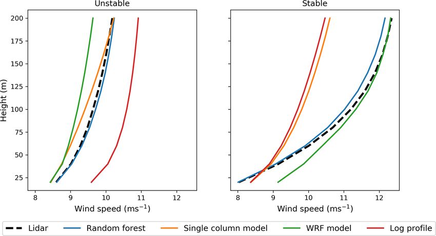
936                                                                 M. Optis et al.: Novel methods for offshore wind extrapolation

Table 1. Active floating lidar deployments in US offshore wind energy areas with publicly available data (as of December 2020).

   Location                                Time         Start date for    Maximum        Data
                                           resolution   public data      measurement     access
                                                                           height
   Hudson South Call Area, New Jersey      1 min        4 Sep 2019           200 m       DNV-GL (2020)
   Hudson North Call Area, New Jersey      10 min       12 Aug 2019          200 m       DNV-GL (2020)
   Atlantic Shores, New Jersey             10 min       26 Feb 2020          250 m       Atlantic Shores Offshore Wind (2020)
   Mayflower, Massachusetts                Daily        13 Apr 2020          250 m       Mayflower Offshore Wind (2020)
   Humboldt, California                    1s           1 Oct 2020           250 m       Pacific Northwest National Laboratory (2020)
   Morro Bay, California                   1s           1 Oct 2020           250 m       Pacific Northwest National Laboratory (2020)

   In place of rotor-swept height measurements, near-surface             occur, which idealized models, such as the logarithmic wind
observations can be used as substitutes for characterizing the           profile, are unable to account for.
offshore wind resource (Mohandes and Rehman, 2018). The                     Despite these shortcomings, the logarithmic profile still
main data source is the network of buoy-based wind speed                 forms the backbone of the only novel extrapolation method
measurements from the National Data Buoy Center, main-                   that has been developed and validated for offshore applica-
tained by the National Oceanic and Atmospheric Adminis-                  tions. This novel method, developed by researchers at the
tration (National Data Buoy Center, 1971). These data have               Technical University of Denmark (DTU) in 2010, derives a
been used to characterize the wind resource in offshore Cali-            stability-dependent long-term correction to the logarithmic
fornia (Wang et al., 2019; Optis et al., 2020c), the US off-             wind profile (Kelly and Gryning, 2010), where stability data
shore Atlantic (Optis et al., 2020b), and the Great Lakes                (e.g., Obukhov length) are provided by numerical weather
(Doubrawa et al., 2015). These buoys generally provide years             prediction simulations. This model (described in more de-
worth of wind speed measurements at heights of less than 5 m             tail in Sect. 3 and herein referred to as the DTU method)
and are of high quality. In addition to these buoys, satellite-          has been used in subsequent studies to extrapolate 10 m di-
based scatterometer and synthetic-aperture radar measure-                agnosed winds from satellite products with good agreement
ments of the near-surface wind vector are increasingly being             with offshore observations in Europe (Badger et al., 2015;
used to characterize the offshore wind resource (Doubrawa                Hasager et al., 2020). The DTU method, however, can pro-
et al., 2015; Ahsbahs et al., 2017; Hasager et al., 2020; Ahs-           vide only a long-term mean wind profile extrapolation and is
bahs et al., 2020). These data are more spatially resolved than          not useful when time-series-based wind speeds across rotor-
buoy-based wind speed data, but they are limited in their tem-           swept heights are needed (i.e., for most energy and economic
poral coverage. Further, there is some error and uncertainty             offshore wind analyses).
in how geophysical transfer functions are used to extrapolate               For such applications, two novel approaches with proven
the satellite measurements to the diagnosed 10 m wind speed              success on land but not thoroughly validated offshore could
that is disseminated (Kelly and Gryning, 2010; Badger et al.,            be suitable. The first is a single-column model (SCM)
2015).                                                                   approach, in which a typical three-dimensional numerical
   This abundance of near-surface wind speed measurements                weather prediction model is reduced to a single vertical di-
is valuable for offshore wind resource characterization pro-             mension by assuming horizontal homogeneity (Baas et al.,
vided the measurements can be accurately extrapolated to                 2010). Further assumptions (described in Sect. 3) reduce the
rotor-swept heights. The conventional wind industry ap-                  model to a simple set of differential equations that can be run
proach – the power-law profile – is not useful in this context           efficiently on a personal computer. The key advantage of the
because the method requires measurements at two heights                  SCM is its ability to be forced at the lower boundary by wind
to calculate the shear coefficient. The logarithmic wind pro-            and temperature observations. The SCM was used in Optis
file (Monin and Obukhov, 1954), by contrast, is applicable               and Monahan (2016) and Optis and Monahan (2017) to ex-
and has a long history of accurately predicting wind speeds              trapolate 10 m wind speeds up to 200 m at the Cabauw mete-
in the atmospheric surface layer (Holtslag, 1984; Troen and              orological tower in the Netherlands. Results showed that the
Petersen, 1989; Emeis, 2013); however, the logarithmic as-               SCM performed about the same as the Weather Research and
sumption has been shown to break down at rotor-swept                     Forecasting (WRF) model (Skamarock et al., 2019) during a
heights under conditions of stable stratification as turbulent           10-year period, highlighting the benefit of local observations
fluxes decrease in magnitude and near-surface winds begin                driving a highly simplified model.
to decouple from the winds aloft (Optis et al., 2014, 2016).                The second novel method is based on machine learning,
Under such conditions, phenomena such as low-level jets can              which has emerged as a promising approach for the vertical
                                                                         extrapolation of wind speeds. Bodini and Optis (2020a) and

Wind Energ. Sci., 6, 935–948, 2021                                                          https://doi.org/10.5194/wes-6-935-2021
M. Optis et al.: Novel methods for offshore wind extrapolation                                                             937

Bodini and Optis (2020b) explored this concept using four li-
dars and surface flux stations dispersed around the Southern
Great Plains site, operated by Argonne National Laboratory.
They found that a relatively simple random forest algorithm,
trained on near-surface atmospheric variables, considerably
outperformed the conventional power-law and logarithmic
wind profiles. This performance held even when a model was
trained at one measurement site and tested at others up to
100 km away, i.e., through a round-robin approach. In the off-
shore environment, Vassallo et al. (2020) used a deep neural
network to extrapolate near-surface winds in offshore Cali-
fornia during a 1-month period, and they also found improve-
ment relative to conventional techniques; however, the time
period was short, and a round-robin approach was not ap-
plied.                                                           Figure 1. WRF simulation domain map considered in this study.
   The goal of this study is to assess the viability of these    The NYSERDA lidars are shown as blue and orange diamonds.
conventional and more novel extrapolation models for use in      White areas denote Bureau of Ocean Energy Management wind en-
US offshore areas. We provide comparisons among the dif-         ergy lease areas; gray areas denote Bureau of Ocean Energy Man-
                                                                 agement call areas.
ferent extrapolation models, and we benchmark against es-
timated wind profiles from the WRF model. We focus this
study on the US North Atlantic and mid-Atlantic offshore ar-
                                                                 dating the extrapolation models alongside WRF will provide
eas, where the US offshore wind industry is most developed
                                                                 key insights into the usefulness of novel extrapolation models
(Musial et al., 2020). In Sect. 2, we describe the domain,
                                                                 for offshore wind energy and whether further development of
the observations, and the WRF model setup used. Next, in
                                                                 these models is justified.
Sect. 3, we describe the various extrapolation models. Inter-
                                                                    A summary of the WRF model setup is provided in Ta-
comparisons of model performance are provided in Sect. 4,
                                                                 ble 3, and the domain is shown in Fig. 1. The WRF model
with concluding remarks provided in Sect. 5.
                                                                 is run from 1 September 2019 through 31 August 2020, in
                                                                 separate monthly runs. For each month, the simulation is ini-
2     Data                                                       tialized 2 d earlier (e.g., 30 March for April simulations) and
                                                                 run 1 d after the end of the month (e.g., 1 May). The first
2.1    Observations                                              day of the simulation is used to spin up the model from ini-
                                                                 tial conditions, whereas the second and final days are used to
To develop and validate the various extrapolation models,
                                                                 stitch together the monthly runs into a single time series.
we leverage measurement data from two recently deployed
floating lidars in offshore New Jersey and located within two
current wind energy call areas (Fig. 1). These lidars were de-   3     Extrapolation models
ployed by the New York State Energy Research and Devel-
opment Authority (NYSERDA), which has made data pub-             In this section we describe the different wind speed extrapo-
licly available in real time through a web-based access portal   lation models considered in this study. We first describe the
(DNV-GL, 2020). The portal also includes detailed techni-        conventional logarithmic wind profile and then discuss the
cal information regarding the lidars. An overview of these       DTU method, which is adopted for this study. We then dis-
floating lidars and the data available are provided in Ta-       cuss the most novel approaches that we have developed ex-
ble 2. Lidar-measured wind speeds from 20 to 200 m are used      plicitly for this study, namely the single-column-model and
for the validation of the proposed extrapolation models (see     machine-learning methods.
Sect. 4), whereas the near-surface measurements at 2 m are
used to develop and apply the extrapolation models (Sect. 3).    3.1    Logarithmic profile
Lidar-measured wind speeds are reported to have an uncer-        The logarithmic wind profile is given as
tainty of 3.3 % (NYSERDA, 2021).
                                                                                          z z
                                                                         u∗      z                 0
                                                                 U (z) =     ln      − ψm       ,      ,                    (1)
2.2    WRF model                                                         κ       z0           L L

The WRF model is used in this study for two reasons. First,      where U is the wind speed, κ is the von Kármán constant
the DTU method (one of the extrapolation approaches con-         (typically taken to be 0.4), z is the height above the sur-
sidered in our analysis) requires surface atmospheric vari-      face, u∗ is the friction velocity, z0 is the roughness length,
ables not available from the NYSERDA buoys. Second, vali-        ψm is the stability function for momentum that adjusts

https://doi.org/10.5194/wes-6-935-2021                                                  Wind Energ. Sci., 6, 935–948, 2021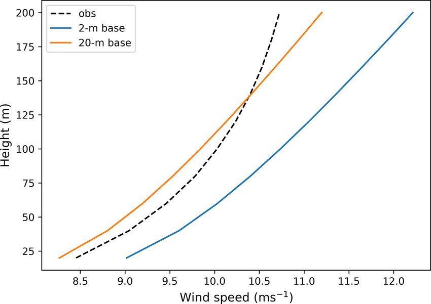
938                                                                          M. Optis et al.: Novel methods for offshore wind extrapolation

Table 2. Summary of observational data set being analyzed.

                                                    Buoy E06                           Buoy E05
            Location                                39.55◦ N, 73.43◦ W           39.97◦ N, 72.72◦ W
            Period analyzed                         4 Sep 2019–16 Aug 2020 12 Aug 2019–16 Aug 2020
            Distance from coast                     69 km                        114 km
            Lidar measurement heights                                         20–200 m in 20 m increments
            Lidar variables                                                    Wind speed, wind direction
            Surface variables                       2 m air temperature, sea surface temperature, 2 m wind speed, 2 m wind direction
            Measured wind speed uncertainty         3.3 %                        3.3 %

Table 3. Key attributes of the WRF model used in this study.

  Feature                           Specification
  WRF version                       4.2.1
  Grid spacing for nested domains   6 km, 2 km
  Output time resolution            5 min
  Vertical levels                   61
  Near-surface-level heights (m)    12, 34, 52, 69, 86, 107, 134, 165, 200
  Atmospheric forcing               ERA5 reanalysis
  Atmospheric nudging               Spectral nudging on 6 km domain, applied every 6 h
  Planetary boundary layer scheme   Mellor–Yamada–Nakanishi–Niino Level 2.5
  Microphysics                      Ferrier
  Longwave radiation                Rapid radiative transfer model
  Shortwave radiation               Rapid radiative transfer model
  Topographic database              Global multiresolution terrain elevation data from the US Geological Survey and National Geospatial-Intelligence Agency
  Land-use data                     Moderate Resolution Imaging Spectroradiometer 30 s
  Cumulus parameterization          Kain–Fritsch

the wind profile depending on atmospheric stability, and                         ture at 2 m, θsurf is the potential temperature at the surface,
L is the Monin–Obukhov length that characterizes surface                         and U2 m is the 2 m wind speed. Combining Eqs. (2) and (3)
layer atmospheric stability. The friction velocity, u∗ , requires                yields the following relationship between L and RiB :
high-frequency sonic anemometer measurements that are not
                                                                                                   z         z z0

available at the NYSERDA buoys. To avoid specifying u∗ ,                                 z    ln  z0 − ψh L , L
we reformulate Eq. (1) to use the 2 m buoy wind speeds as a                      RiB = h                        i 2 ,                     (4)
                                                                                         L
reference measurement, allowing the wind profile to be cal-                                  ln zz0 − ψm Lz , zL0
culated according to
                                                                               where ψh is the stability function for temperature, also taken
                   ln (z/z0 ) − ψm (z/L, z0 /L)                                  from Jiménez et al. (2012).
U (z) = U2 m                                           .      (2)
                ln (zref /z0 ) − ψm (z2 m /L, z0 /L)                                Using Eq. (4), we iteratively solve for L given RiB , which
                                                                                 combined with Eq. (2) allows for the calculation of the verti-
Here, we set z0 = 0.0001 (which is the WRF output z0 for                         cal wind profile.
offshore) and implement the ψm formulations from Jiménez
et al. (2012), which have become standard correction func-
                                                                                 3.2    DTU model
tions and are currently used in the WRF mesoscale model
surface layer parameterization.                                                  Noting the breakdown of the logarithmic wind profile in very
   The calculation of L typically requires measurements of                       stable conditions, the DTU method aims to preserve its ap-
the momentum and turbulent temperature fluxes, which are                         plicability by applying it only in the context of a mean long-
not available from buoy measurements but require high-                           term wind profile, which is generally well estimated as log-
frequency three-dimensional wind speed components and                            arithmic. The overall approach is to account for the distri-
temperature measurements. Instead, we can calculate a                            bution of L value output from WRF throughout the year. As
“bulk” L based on the bulk Richardson number, RiB :                              such, the DTU method is suitable only for long-term wind re-
         g z (θz − θsurf )                                                       source assessment because it requires at least 1 year of data
RiB =                      ,                                           (3)       and ideally many years (Kelly and Gryning, 2010).
        θavg     Uz2
                                                                                    The stability correction applied to the log extrapolation
where z is the height 2 m above the surface, g is the accel-                     is height-dependent and computed based on empirical con-
eration as a result of gravity, θz2 m is the potential tempera-                  stants and atmospheric conditions at the site: the percentage

Wind Energ. Sci., 6, 935–948, 2021                                                                       https://doi.org/10.5194/wes-6-935-2021
M. Optis et al.: Novel methods for offshore wind extrapolation 939
Figure 2. Schematic of quantities and calculations involved in the DTU model considered herein.
of stable vs. unstable conditions; the quadratic mean of the
kinematic heat flux; the mean, near-surface air temperature;
and the time-averaged friction velocity. These input parame-
ters are taken from the WRF simulations and are combined
with stability functions, ψm , based on similarity theory to
compute a vertical profile of the correction function (Fig. 2).
This correction is then added to the log extrapolation to yield
a wind speed profile, as in Eq. (1), where u∗ is taken from the
WRF simulation, and z0 is computed using the Charnock re-
lationship, z0 = αu2∗ /g, with g being the acceleration caused
by gravity, and α = 0.0144 (Charnock, 1955).
Before implementing this model, we verify that the prob-
ability distribution functions for atmospheric stability are a
good fit to the empirical distributions. This comparison is
given in Fig. 3. The functions shown in this figure take into
account the percentage of stable vs. unstable conditions at
the NYSERDA buoy sites (nstable and nunstable ), scales of Figure 3. Empirical vs. theoretical distribution of atmospheric sta-
variation for L−1 (σstable and σunstable ), and empirical con- bility for the two buoy sites.
stants (Cstable = 5 and Cunstable = 12). Note that previous
work focusing on other data sets used different values for
the C± constants (e.g., both were set to 3.0 in Badger et al., and air temperature; the sea surface temperature and air–sea
2015, to extrapolate satellite-derived wind speed measure- temperature difference; and the time of day and month of
ments). year. Wind direction, time of day, and month of year are all
decomposed into their sine and cosine components to pre-
serve circularity (i.e., 0 and 360◦ directions are equivalent,
3.3 Random forest machine-learning model
as are 00:00 and 24:00 LT)1 . A summary of these variables is
The third model considered is based on machine learning. listed in Table 4.
Here, we consider a relatively simple ensemble-based re- To ensure that the observation sets over which the random
gression tree method, known as a random forest model, forest is trained and tested cover as much of the seasonal vari-
which has shown strong predictive power in previous land- ability as possible, we build the testing set using a consecu-
based wind speed extrapolation work (Bodini and Optis, tive 20 % of the observations from each month in the period
2020a, b) and in relating wind plant energy production to on- of record. We evaluate 20 randomly selected combinations
site atmospheric variables (Optis and Perr-Sauer, 2019). We of the hyperparameters with a fivefold cross-validation. The
use the RandomForestRegressor module in Python’s hyperparameters considered in the cross-validation and their
Scikit-learn (Pedregosa et al., 2011). We consider a range
of 10 min averaged input variables available from the NY- 1 Both are needed because each value of sine only (or cosine
SERDA buoys: 2 m wind speed, wind direction, pressure, only) is linked to two different values of the cyclical feature.
https://doi.org/10.5194/wes-6-935-2021 Wind Energ. Sci., 6, 935–948, 2021940 M. Optis et al.: Novel methods for offshore wind extrapolation
Table 4. Input features used for the random forest model. ods and that no model has prior knowledge of lidar-measured
wind profiles at the site where it is evaluated.
Input feature Acronym Measurement
height 3.4 Single-column model
(m a.g.l.)
The fourth model considered is an SCM. Essentially, it is a
2 m wind speed WS 2 m 2
stripped-down version of a three-dimensional model, such as
Sine of 2 m wind direction WRF, in which only vertical exchanges are considered and
WD 2
Cosine of 2 m wind direction horizontal homogeneity is assumed. This greatly simplifies
2 m air temperature T 2 the governing equations of a three-dimensional model and
reduces the SCM to a one-dimensional model in the verti-
Sea surface temperature SST 0 cal direction. By assuming no moisture or cloud radiation,
Air–sea temperature difference T –SST – the equations of motion simplify further and depend only on
the horizontal pressure gradients, the Coriolis force, and the
2 m air pressure p 2
vertical turbulent flux of momentum and temperature:
Sine of time of the day
Time – ∂u ∂(u0 w 0 )
Cosine of time of the day = f (v − vG ) − ,
∂t ∂z
Sine of month
Month – ∂v ∂(v 0 w0 )
Cosine of month = f (u − uG ) − ,
∂t ∂z
∂θ ∂(θ 0 w0 )
Table 5. Algorithm hyperparameters sampled in the random forest = , (5)
∂t ∂z
cross-validation.
where u, v, and w are the three vector wind components; t is
Hyperparameter Possible time; z is the height above the surface; θ is potential tem-
values perature; and uG and vG are the u and v components of the
Number of estimators 10–800 geostrophic wind. The u0 w0 , v 0 w 0 terms represent the u and
Maximum depth 4–40 v components of the vertical turbulent momentum flux, and
Maximum number of features 1–11 θ 0 w0 represents the vertical turbulent temperature flux.
Minimum number of samples to split 2–11 The momentum and temperature fluxes are not solved di-
Minimum number of samples for a leaf 1–15 rectly but rather parameterized based on well-established
eddy–diffusivity relationships:
∂u
u0 w 0 = −Km ,
sampled ranges are shown in Table 5. We evaluate the per- ∂z
formance of the learning algorithm based on the root-mean- ∂v
square error (RMSE) between the measured and predicted v 0 w 0 = −Km ,
∂z
wind speed at extrapolation height: the set of hyperparame- ∂θ
ters that leads to the lowest RMSE is selected and used to θ 0 w0 = −Kh , (6)
∂z
assess the final performance of the learning algorithm.
As described in detail in Bodini and Optis (2020b), it is where Km and Kh are the eddy diffusivities for momentum
both impractical and unfair to evaluate a machine-learning and temperature, respectively. These terms are themselves
model at the same site where it is trained. Critically, the parameterized with a range of possible options in the litera-
model requires observations of the lidar-measured wind ture (Optis and Monahan, 2016, 2017). We adopt a relatively
speeds up to 200 m to be trained. Evaluating model perfor- simple first-order closure model that includes eddy diffusivi-
mance at the training site is impractical because the wind ties that are related to the wind speed gradient and a stability
profiles are already known and unfair because the other ex- function that depends on the Richardson number:
trapolation methods do not have such knowledge of lidar- 2 ∂U
measured wind profiles. Instead, model performance must be Km = lm fm (Ri ) ,
∂z
assessed through a round-robin approach, in which the model
is evaluated at a site not used to train the model. Specifically,
∂U
in this study, the random forest model is trained on data at Kh = lm lh fh (Ri ) , (7)
NYSERDA buoy E05 and then evaluated against other ex- ∂z
trapolation models at NYSERDA buoy E06, located 83 km where lm and lh are the mixing lengths for momentum and
away, and then vice versa. This round-robin approach en- temperature, respectively, and fm and fh are the stabil-
sures a fair comparison of the different extrapolation meth- ity functions for momentum and temperature, respectively.
Wind Energ. Sci., 6, 935–948, 2021 https://doi.org/10.5194/wes-6-935-2021M. Optis et al.: Novel methods for offshore wind extrapolation 941
There are a range of proposed formulations for the mixing Table 6. The 10 MW offshore reference wind turbine specifications
lengths and stability functions. Here, we use the one devel- from Beiter et al. (2020) used to calculate REWS.
oped by Smith (1990), which showed strong results when
used in an SCM in previous studies (Optis and Monahan, Characteristic Value
2016, 2017). A detailed explanation and the equations of the Rated power 10 MW
stability functions and mixing lengths can be found in Smith Rotor diameter 196 m
(1990), Cuxart et al. (2006), and Optis and Monahan (2017). Hub height 128 m
The SCM equations are solved on a logarithmically Rotor-swept heights 30–226 m
stretched grid from a height of 2–2000 m with 200 grid
levels that provide higher resolution near the surface. The
lower boundary conditions at 2 m are the measured wind
speed components and temperature from the NYSERDA rotor-equivalent wind speed (REWS) rather than an assumed
buoys. The upper boundary conditions are the 800 hPa hub-height wind speed. Details for calculating REWS are
pressure-level data provided by the ERA5 reanalysis. A zero- provided in Wagner et al. (2014). To calculate REWS, we
temperature gradient boundary condition is also applied at assume a 10 MW offshore reference turbine as described in
the top of the domain. Beiter et al. (2020) and summarized in Table 6.
Recognizing that the geostrophic wind can change with We also assess model performance using the four recom-
height in conditions of horizontal temperature gradients, we mended performance metrics from Optis et al. (2020a), sum-
calculate a geostrophic wind profile at each time step to marized in Table 7. We note that the DTU method is ca-
force the simulations. This is done by first assuming that the pable of modeling only the mean wind profile; therefore,
800 hPa winds from ERA5 are geostrophic, which is a rea- time-series-based performance analysis throughout this sec-
sonable assumption at 2000 m, where surface friction effects tion excludes the DTU method.
should be negligible. Next, we calculate the geostrophic wind We begin with a comparison of the mean wind profile
at the surface using surface pressure and air temperature data in Fig. 4, showing results at both NYSERDA buoys E05
from the ERA5 reanalysis product: and E06. The observed wind profile shows moderate shear,
increasing from approximately 8.5 to 10.5 m s−1 at E05
1 ∂P and 8.0 to 10.3 m s−1 at E06. As shown, the random forest
uG = − ,
fρ ∂y machine-learning model provides excellent agreement with
1 ∂P the mean profile, whereas the other models are deficient in
vG = , (8)
fρ ∂x some respects. The SCM underestimates wind speeds at E05
but is very close to the observed profile at E06. The loga-
where ρ is air density, and P is pressure. The horizontal pres- rithmic profile captures the upper winds relatively well with
sure gradient terms are calculated by taking a planar best fit a slight positive bias, but it has increasingly higher bias at
of the closest nine ERA5 grid points that surround the buoy lower heights. The DTU method significantly overestimates
locations. Equation (8) is used to calculate the geostrophic wind speeds, especially at the upper heights, with nearly a
wind components at 2 m, and finally the geostrophic wind 1.5 m s−1 bias at 200 m. Finally, we see that the WRF model
profile is found by linearly interpolating the 2 m and 800 hPa tends to underestimate the wind profile.
values to the different SCM heights. REWS-based performance metrics for the different mod-
To initialize the simulation, we start by solving for the neu- els are shown in Fig. 5. Again, the strong performance of
tral vertical wind profile by imposing an equilibrium condi- the machine-learning model is apparent, with considerably
tion (i.e., ∂u/∂t = 0; ∂v/∂t = 0; ∂(θ 0 w0 )/∂z = 0). The simu- lower error metrics and higher correlation to observations
lation then moves forward from the neutral profile as a time- relative to the other models. The bias is notably negligible at
marching algorithm using the complete set of equations pro- buoy E05 and slightly negative at E06. In contrast, the SCM
vided in this section. A continuous simulation is launched for has the weakest performance across all metrics at E05 and all
the whole year of measurements without interruption. but the bias at E06. The logarithmic profile performance falls
in between the machine-learning model and the SCM and is
4 Results the only model with a positive bias at both buoys. Finally,
the WRF model tends to perform similarly to the logarith-
The four vertical extrapolation models presented in the pre- mic model, with slightly lower unbiased RMSE and higher
vious section are all validated against lidar data from NY- correlation but higher magnitude of bias and earth mover’s
SERDA buoys E05 and E06 during the full period of record. distance (EMD).
For each lidar, we consider only the time periods where wind Next, we consider the role of atmospheric stability in rela-
speeds are reported at every height from 20–200 m. Based tive model performance. Here, we distinguish between un-
on recent best-practice recommendations for validating off- stable and stable conditions using the WRF-modeled bulk
shore wind models (Optis et al., 2020a), we validate the Richardson number, RiB , between 200 m and the surface
https://doi.org/10.5194/wes-6-935-2021 Wind Energ. Sci., 6, 935–948, 2021942 M. Optis et al.: Novel methods for offshore wind extrapolation
Table 7. Performance metrics used to assess extrapolation model performance.
Name Abbreviation Description
Bias Bias Difference between the mean modeled and observed
result
Unbiased RMSE cRMSE The random error component after bias is removed,
describing the differences in model variations around
the mean
Square of correlation R2 The correspondence or pattern between the modeled
coefficient and observed variable
Earth mover’s distance EMD Difference between the probability distributions
between the modeled and observed variable
Figure 4. Mean modeled and observed wind profiles at NYSERDA buoys E05 and E06. The dotted line denotes the observed profile, and
solid colors denote the different extrapolation models.
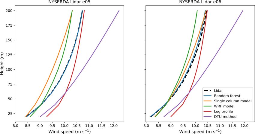
(RiB < 0 for unstable conditions; RiB > 0 for stable condi- relative performance between models at buoy E06. We also
tions). Mean wind profiles by stability regime are shown in see the random forest with the strongest performance met-
Fig. 6. Here, we focus only on buoy E05 and note that relative rics, apart from slightly higher magnitude bias and higher
performance is similar at both buoys. The machine-learning EMD in stable conditions relative to the WRF model. The
model shows similar performance in unstable and stable con- SCM shows lower magnitude bias and EMD in unstable rel-
ditions, accurately capturing the unstable profile and slightly ative to stable conditions but high unbiased RMSE and cor-
underestimating the stable profile. The SCM performs rea- relation across both regimes. The log profile performs better
sonably well in unstable conditions but is unable to capture in unstable conditions than stable conditions for all perfor-
the high shear in the stable regime and significantly underes- mance metrics, whereas the WRF model cRMSE and R 2 are
timates wind speeds. The log profile similarly underestimates lower in unstable conditions, but bias and EMD are higher
wind speeds in stable conditions but overestimates in unsta- relative to stable conditions.
ble conditions. Finally, the WRF model underestimates the Next, we present 12-by-24 heat maps to show the com-
wind profile in unstable conditions while accurately captur- bined diurnal and monthly trends of model performance. We
ing winds greater than 100 m in stable conditions but overes- show only the bias heat maps in Fig. 8. We see that the
timating them when less than 100 m. Overall, we see that all machine-learning model has consistently low magnitude bias
models apart from the random forest struggle with consistent throughout the diurnal and monthly cycles, with no clear di-
accuracy across stability regimes. urnal trends but a tendency to overestimate wind speeds in
This relative consistency is further illustrated in Fig. 7, the fall. The SCM shows considerable negative bias through-
which shows the REWS performance metrics by stability out the year, with a tendency to overestimate wind speeds
regime. Again, we focus on buoy E05 and note the similar in November. Interestingly, the bias in December is pos-
Wind Energ. Sci., 6, 935–948, 2021 https://doi.org/10.5194/wes-6-935-2021M. Optis et al.: Novel methods for offshore wind extrapolation 943
Figure 5. REWS performance metrics for the different vertical extrapolation models.
Figure 6. Mean modeled and observed wind profiles at NYSERDA buoy E05 in unstable (left panels) and stable (right panels) atmospheric
conditions.
itive from 01:00 to 12:00 LT and negative form 13:00 to 4.1 Explaining DTU model performance
00:00 LT. The WRF model shows some trends, with positive
bias in spring in the early hours and negative bias in the mid-
Figure 4 showed that the DTU method significantly over-
dle hours. Finally, the logarithmic profile shows substantial
estimated wind speeds. This is a surprising result given its
trends, with strong overestimation of winds through most of
strong performance in Badger et al. (2015), in which 10 m
the year and underestimation in spring, with the largest mag-
satellite-measured winds were extrapolated. To explore this,
nitude of the underestimates in the early hours.
we compare DTU model performance using both 2 and 20 m
https://doi.org/10.5194/wes-6-935-2021 Wind Energ. Sci., 6, 935–948, 2021944 M. Optis et al.: Novel methods for offshore wind extrapolation
Figure 7. REWS performance metrics for the different vertical extrapolation models at NYSERDA buoy E05 for unstable and stable condi-
tions.
measurements as the basis for extrapolation. The results are air–sea temperature difference at nearly 20 %. This is an im-
shown in Fig. 9. The extrapolation from the 2 m measure- portant result and highlights the influence of atmospheric sta-
ments does not match the measured wind speed profile. This bility on offshore wind profiles.
is likely because the measurement height is too low and lo- In fact, Debnath et al. (2020) found that a positive air–sea
cated within the viscous sublayer, where log-law approxima- temperature difference was the key driver in the observed
tions are not valid. When the same method is used to extrapo- frequent occurrences of extreme wind shear and low-level
late from the 20 m lidar measurements, we see a good match jet events at the E05 and E06 buoys. Table 8 shows that in-
between the extrapolated and measured values. This analysis cluding the air–sea temperature difference results in consid-
reveals that the DTU method is not suitable for extrapolation erable improvements in random forest model performance,
based on buoy wind speed measurements, which are often especially during the extreme high-shear cases identified in
made with propeller or cup anemometers between 2 and 5 m Debnath et al. (2020). Notably, the bias and EMD are both
above the sea surface. Instead, this method should be applied halved for the high-shear cases when using the air–sea tem-
to short offshore meteorological masts and satellite-derived perature difference as an input feature.
wind speed estimates. Finally, we examine how random forest model perfor-
mance using the default round-robin approach (i.e., model
trained and tested at different buoys) compares to that when
4.2 Feature importance in the random forest
trained and tested at the same site. In general, the model
Finally, we examine the random forest model in more detail should perform best when tested at the training site, as was
given its strong performance in this study. Figure 10 shows found in Bodini and Optis (2020b). The degree of model de-
the relative feature importance for each variable used to train terioration with distance can provide insight into how well
the random forest model. Feature importance for the random the model can generalize across space to perform extrapola-
forest model is calculated based on how many times the al- tion. The results of this comparison are shown in Table 9.
gorithm uses the variable to split the data, weighted by the Interestingly, at each site and for each metric, the round-
improvement in model performance because of the split. Not robin performance is slightly better than the same-site perfor-
surprisingly, the 2 m wind speed is the most important fea- mance. Accounting for the fact that the limited 1-year analy-
ture (nearly 80 %). The second most important feature is the sis contributes to some uncertainty in these metrics, it is clear
Wind Energ. Sci., 6, 935–948, 2021 https://doi.org/10.5194/wes-6-935-2021M. Optis et al.: Novel methods for offshore wind extrapolation 945
Figure 8. Heat maps (12 by 24) of REWS bias at NYSERDA buoy E05 for the different extrapolation models.
Figure 10. Relative feature importance for the random forest model
Figure 9. Mean observed and modeled wind profiles at NYSERDA in predicting 120 m wind speeds at NYSERDA buoy E05.
buoy E05 when using the DTU method based on 2 and 20 m mea-
surements.
which can be attributed to the horizontal homogeneity of the
offshore environment – has important implications for the ap-
that there is at best negligible model degradation through- plicability of machine-learning extrapolation techniques for
out an offshore distance of 83 km. In contrast, Bodini and all US offshore waters using only a handful of lidar training
Optis (2020b) found that, on land, model performance de- sites.
creased with distance from the training site, ranging from
11 %–14 % reductions throughout distances ranging between
40–100 km. The negligible performance reduction offshore –
https://doi.org/10.5194/wes-6-935-2021 Wind Energ. Sci., 6, 935–948, 2021946 M. Optis et al.: Novel methods for offshore wind extrapolation
Table 8. Performance metrics at buoy E05 for the random sults. Improving the SCM design to account for atmospheric
forest model with and without the air–sea temperature differ- stability (e.g., by substituting the temperature lower bound-
ence (1Tair–sea ) as an input feature. ary condition with a flux-based measurement) should be an
area of future work.
Metric All data High-shear cases Results from this study clearly show the promise of a
Without With Without With machine-learning-based approach to offshore wind extrapo-
1Tair–sea 1Tair–sea 1Tair–sea 1Tair–sea lation. It seems likely that models trained on only a handful
Bias (m s−1 ) 0.03 0.04 −1.05 −0.58 of lidars dispersed in offshore waters could be sufficient to
cRMSE (m s−1 ) 1.07 0.84 1.46 1.29 accurately extrapolate wind speeds at all offshore locations
EMD (m s−1 ) 0.19 0.12 1.05 0.58 in the surrounding area where surface measurements exist.
R2 0.95 0.97 0.89 0.91 This hypothesis should be tested more thoroughly using the
additional floating lidars recently deployed in US waters (Ta-
Table 9. Comparison of random forest model performance when ble 1). The ability for a machine-learning model to generalize
trained and tested under a round-robin vs. a same-site approach. across different oceans in particular (e.g., training a model in
the Atlantic and testing it in the Pacific) would be an impor-
Metric Buoy E05 Buoy E06 tant area of future work as the US offshore wind industry
looks to Hawaii, the Pacific Northwest, and the Great Lakes
Round Same Round Same
for future expansion (Musial et al., 2020).
robin site robin site
Applying the machine-learning approach to satellite-based
Bias (m s−1 ) 0.07 −0.09 −0.05 −0.02 wind speed observations would be the next future area of
cRMSE (m s−1 ) 0.86 0.94 0.89 0.94 study. A collaboration between the National Renewable En-
EMD (m s−1 ) 0.13 0.16 0.09 0.13 ergy Laboratory and DTU resulted in a US Atlantic wind
R2 0.97 0.96 0.96 0.96 atlas at 10 m a.s.l. (above sea level) (Ahsbahs et al., 2020).
Training and evaluating a machine-learning model at floating
lidar sites using only data available across all the US Atlantic
5 Conclusions area (i.e., satellite-measured winds and sea surface tempera-
ture) would provide key insights into whether the Ahsbahs
In this study, we developed novel methods for the vertical ex- et al. (2020) wind atlas could be accurately extrapolated
trapolation of near-surface offshore wind speeds. We evalu- across offshore wind turbine rotor-swept heights.
ated these methods against conventional extrapolation meth- This proposed scope of future research will be aided by
ods and WRF-modeled wind speeds using two floating li- continued efforts to make floating lidar data public. Most de-
dars deployed in US Atlantic wind energy call areas during ployed lidars are currently owned by wind energy develop-
a 1-year period. Of the four wind speed vertical extrapola- ers and not publicly available. Public access to these data
tion models considered, the random forest machine-learning would greatly improve our understanding of the US offshore
model significantly outperformed the other models and ac- wind resource and help produce more accurate hub-height
curately represented winds across the vertical profile in dif- observation-based offshore wind atlases.
ferent seasons and times of day and in different stability
regimes. Further, the random forest model substantially out-
performed the WRF model, highlighting the benefit of local Code and data availability. Observational data from the floating
observations in generating wind profiles. Moreover, the ran- lidars are publicly available at DNV-GL (2020). The open-source
dom forest model showed negligible to no performance de- WRF model was used for the numerical weather prediction simula-
crease throughout the 83 km distance between the two float- tions.
ing lidars.
The SCM performance offshore could be improved con-
Author contributions. MO wrote the manuscript, conducted the
siderably through better accounting of near-surface stabil-
WRF simulations, and performed the inter-model comparison.
ity. The model was forced at its lower boundary only by
NB built the random forest model and wrote Sect. 3.3, MD built
the 2 m wind speed and temperature and critically did not the SCM model and wrote Sect. 3.4, and PD built the DTU model
consider the role of sea surface temperature and related heat and wrote Sect. 3.2.
flux; therefore, the SCM really had no way to account for
or to characterize the role of atmospheric stability, which
was demonstrated in this study to be an important driver of Competing interests. The authors declare that they have no con-
the wind profile. In contrast, the WRF model can capture flicts of interest.
these effects, and the machine-learning model used the air–
sea temperature difference, a proxy for atmospheric stability,
as an input variable, which considerably improved model re-
Wind Energ. Sci., 6, 935–948, 2021 https://doi.org/10.5194/wes-6-935-2021M. Optis et al.: Novel methods for offshore wind extrapolation 947
Acknowledgements. This work was supported and funded by the Cuxart, J., Holtslag, A. A. M., Beare, R. J., Bazile, E., Beljaars,
Bureau of Ocean Energy Management. We would like to thank An- A., Cheng, A., Conangla, L., Ek, M., Freedman, F., Hamdi, R.,
gel McCoy specifically for her support and guidance throughout Kerstein, A., Kitagawa, H., Lenderink, G., Lewellen, D., Mail-
this work. We also thank NYSERDA and DNV-GL for making the hot, J., Mauritsen, T., Perov, V., Schayes, G., Steeneveld, G.-J.,
two floating lidar data publicly available, without which this study Svensson, G., Taylor, P., Weng, W., Wunsch, S., and Xu, K.-
would not have been possible. M.: Single-Column Model Intercomparison for a Stably Strati-
fied Atmospheric Boundary Layer, Bound.-Lay. Meteorol., 118,
273–303, https://doi.org/10.1007/s10546-005-3780-1, 2006.
Financial support. This research has been supported by the Bu- Debnath, M., Doubrawa, P., Optis, M., Hawbecker, P., and Bodini,
reau of Ocean Energy Management (grant no. IAG-19-2122). N.: Extreme Wind Shear Events in US Offshore Wind Energy
Areas and the Role of Induced Stratification, Wind Energ. Sci.
Discuss. [preprint], https://doi.org/10.5194/wes-2020-103, in re-
Review statement. This paper was edited by Joachim Peinke and view, 2020.
reviewed by two anonymous referees. DNV-GL: NYSERDA Floating LiDAR Buoy Data, available at:
https://oswbuoysny.resourcepanorama.dnvgl.com/ (last access:
28 February 2021), 2020.
Doubrawa, P., Barthelmie, R. J., Pryor, S. C., Hasager, C.
References B., Badger, M., and Karagali, I.: Satellite winds as a
tool for offshore wind resource assessment: The Great
Ahsbahs, T., Badger, M., Karagali, I., and Larsén, X. G.: Lakes Wind Atlas, Remote Sens. Environ. 168, 349–359,
Validation of Sentinel-1A SAR Coastal Wind Speeds https://doi.org/10.1016/j.rse.2015.07.008, 2015.
Against Scanning LiDAR, Remote Sens., 9, 552–569, Emeis, S.: Wind Energy Meteorology, Springer, Dordrecht, 2013.
https://doi.org/10.3390/rs9060552, 2017. Hasager, C. B., Madsen, P. H., Giebel, G., Réthoré, P.-E., Hansen,
Ahsbahs, T., Maclaurin, G., Draxl, C., Jackson, C. R., Monaldo, K. S., Badger, J., Pena Diaz, A., Volker, P., Badger, M., Karagali,
F., and Badger, M.: US East Coast synthetic aperture radar wind I., Cutululis, N. A., Maule, P., Schepers, G., Wiggelinkhuizen,
atlas for offshore wind energy, Wind Energ. Sci., 5, 1191–1210, J., Cantero, E., Waldl, I., Anaya-Lara, O., Attya, A. B., Svend-
https://doi.org/10.5194/wes-5-1191-2020, 2020. sen, H., Palomares, A., Palma, J., Gomes, V. C., Gottschall, J.,
Atlantic Shores Offshore Wind: Atlantic Shores Floating Li- Wolken-Möhlmann, G., Bastigkeit, I., Beck, H., Trujillo, J.-J.,
DAR Buoy Data, available at: https://erddap.maracoos.org/ Barthelmie, R., Sieros, G., Chaviaropoulos, T., Vincent, P., Hus-
erddap/tabledap/AtlanticShores_ASOW-4_wind.html (last ac- son, R., and Prospathopoulos, J.: Design tool for offshore wind
cess: 11 June 2021), 2020. farm cluster planning, in: Proceedings of the EWEA Annual
Baas, P., Bosveld, F., Lenderink, G., van Meijgaard, E., and Holt- Event and Exhibition 2015, EWEA – European Wind Energy As-
slag, A. A. M.: How to design single-column model experiments sociation, Paris, France, 2015.
for comparison with observed nocturnal low-level jets, Q. J. Roy. Hasager, C. B., Hahmann, A. N., Ahsbahs, T., Karagali, I., Sile, T.,
Meteorol. Soc., 136, 671–684, https://doi.org/10.1002/qj.592, Badger, M., and Mann, J.: Europe’s offshore winds assessed with
2010. synthetic aperture radar, ASCAT and WRF, Wind Energ. Sci., 5,
Badger, M., Peña, A., Hahmann, A. N., Mouche, A. A., and 375–390, https://doi.org/10.5194/wes-5-375-2020, 2020.
Hasager, C. B.: Extrapolating Satellite Winds to Turbine Holtslag, A. A. M.: Estimates of diabatic wind speed profiles from
Operating Heights, J. Appl. Meteorol. Clim., 55, 975–991, near-surface weather observations, Bound.-Lay. Meteorol., 29,
https://doi.org/10.1175/JAMC-D-15-0197.1, 2015. 225–250, https://doi.org/10.1007/BF00119790, 1984.
Beiter, P., Musial, W., Duffy, P., Cooperman, A., Shields, M., Jiménez, P. A., Dudhia, J., González-Rouco, J. F., Navarro, J., Mon-
Heimiller, D., and Optis, M.: The Cost of Floating Offshore Wind távez, J. P., and García-Bustamante, E.: A Revised Scheme for
Energy in California Between 2019 and 2032, NREL, Golden, the WRF Surface Layer Formulation, Mon. Weather Rev., 140,
Colorado, USA, https://doi.org/10.2172/1710181, 2020. 898–918, https://doi.org/10.1175/MWR-D-11-00056.1, 2012.
Bodini, N. and Optis, M.: How accurate is a machine learning- Jong, P., Dargaville, R., Silver, J., Utembe, S., Kiperstok, A., and
based wind speed extrapolation under a round-robin approach?, Torres, E. A.: Forecasting high proportions of wind energy sup-
J. Phys.: Conf. Ser., 1618, 062037, https://doi.org/10.1088/1742- plying the Brazilian Northeast electricity grid, Appl. Energy,
6596/1618/6/062037, 2020a. 195, 538–555, https://doi.org/10.1016/j.apenergy.2017.03.058,
Bodini, N. and Optis, M.: The importance of round-robin val- 2017.
idation when assessing machine-learning-based vertical ex- Kelly, M. and Gryning, S.-E.: Long-Term Mean Wind Profiles
trapolation of wind speeds, Wind Energ. Sci., 5, 489–501, Based on Similarity Theory, Bound.-Lay. Meteorol., 136, 377–
https://doi.org/10.5194/wes-5-489-2020, 2020b. 390, https://doi.org/10.1007/s10546-010-9509-9, 2010.
Carbon Trust: Carbon Trust Offshore Wind Accelerator Mahoney, W. P., Parks, K., Wiener, G., Liu, Y., Myers, W. L.,
Roadmap, Tech. rep., available at: https://prod-drupal-files. Sun, J., Delle Monache, L., Hopson, T., Johnson, D., and
storage.googleapis.com/documents/resource/public/ Haupt, S. E.: A Wind Power Forecasting System to Opti-
owa-w-uflr-updated-fl-roadmap_18102018.pdf (last access: mize Grid Integration, IEEE T. Sustain. Energ., 3, 670–682,
10 March 2021), 2018. https://doi.org/10.1109/TSTE.2012.2201758, 2012.
Charnock, H.: Wind stress on a water surface, Q. J. Roy. Meteo- Mayflower Offshore Wind: Mayflower Floating LiDAR Buoy Data,
rol. Soc., 81, 639–640, https://doi.org/10.1002/qj.49708135027, available at: http://www.neracoos.org/erddap/tabledap/SHELL_
1955.
https://doi.org/10.5194/wes-6-935-2021 Wind Energ. Sci., 6, 935–948, 2021948 M. Optis et al.: Novel methods for offshore wind extrapolation MAYFLOWER_winds_csv_all.html (last access: 15 Febru- Optis, M., Kumler, A., Scott, G., Debnath, M., and Moriarty, P.: Val- ary 2021), 2020. idation of RU-WRF, the Custom Atmospheric Mesoscale Model Mohandes, M. A. and Rehman, S.: Wind speed ex- of the Rutgers Center for Ocean Observing Leadership, re- trapolation using machine learning methods and Li- port no. NREL/TP-5000-75209, NREL, Golden, Colorado, USA, DAR measurements, IEEE Access, 6, 77634–77642, p. 61, https://doi.org/10.2172/1599576, 2020b. https://doi.org/10.1109/ACCESS.2018.2883677, 2018. Optis, M., Rybchuk, O., Bodini, N., Rossol, M., and Musial, W.: Monin, A. and Obukhov, A.: Basic Laws of Turbulent Mixing in the 2020 Offshore Wind Resource Assessment for the California Pa- Surface Layer of the Atmosphere, Contrib. Geophys. Inst. Acad. cific Outer Continental Shelf, Tech. Rep. NREL/TP-5000-77642, Sci., 24, 163–187, 1954. NREL – National Renewable Energy Laboratory, Golden, CO, Musial, W., Beiter, P., Nunemaker, J., Gevorgian, V., Cooper- USA, https://doi.org/10.2172/1677466, 2020c. man, A., Hammond, R., Shields, M., and Spitsen, P.: 2019 Off- Pacific Northwest National Laboratory: Buoy Lidar Data, Cal- shore Wind Technology Data Update, Tech. Rep. NREL/TP- ifornia, available at: https://a2e.energy.gov/data?ProjectFilter= 5000-77411, 1677477, MainId:26357, NREL, Golden, Col- ["buoy"5D] (last access: 10 May 2021), 2020. orado, USA, https://doi.org/10.2172/1677477, 2020. Pedregosa, F., Varoquaux, G., Gramfort, A., Michel, V., Thirion, National Data Buoy Center: Meteorological and oceanographic data B., Grisel, O., Blondel, M., Prettenhofer, P., Weiss, R., Dubourg, collected from the National Data Buoy Center Coastal-Marine V., Vanderplas, J., Passos, A., Cournapeau, D., Brucher, M., Per- Automated Network (C-MAN) and moored (weather) buoys, rot, M., and Duchesnay, E.: Scikit-learn: Machine Learning in available at: https://www.ndbc.noaa.gov/ (last access: 10 Febru- Python, J. Mach. Learn. Res., 12, 2825–2830, 2011. ary 2021), 1971. Skamarock, C., Klemp, B., Dudhia, J., Gill, O., Liu, Z., Berner, J., NYSERDA: Hudson North and Hudson South Call Areas Off- Wang, W., Powers, G., Duda, G., Barker, D., and Huang, X.-Y.: shore Wind Farm Energy Assessment Report, Tech. rep., avail- A Description of the Advanced Research WRF Model Version 4, able at: https://oswbuoysny.resourcepanorama.dnvgl.com/, last NCAR, Boulder, Colorado, USA, https://doi.org/10.5065/1dfh- access: 15 March 2021. 6p97, 2019. Optis, M. and Monahan, A.: The Extrapolation of Near-Surface Smith, R. N. B.: A scheme for predicting layer clouds and their wa- Wind Speeds under Stable Stratification Using an Equilibrium- ter content in a general circulation model, Q. J. Royal Meteorol. Based Single-Column Model Approach, J. Appl. Meteorol. Clim. Soc., 116, 435–460, https://doi.org/10.1002/qj.49711649210, 55, 923–943, https://doi.org/10.1175/JAMC-D-15-0075.1, 2016. 1990. Optis, M. and Monahan, A.: A Comparison of Equilibrium and Troen, I. and Petersen, E.: European Wind Atlas, Riso National Lab- Time-Evolving Approaches to Modeling the Wind Profile under oratory, Roskilde, 1989. Stable Stratification, J. of Appl. Meteorol. Clim., 56, 1365–1382, Vassallo, D., Krishnamurthy, R., and Fernando, H. J. S.: Decreas- https://doi.org/10.1175/JAMC-D-16-0324.1, 2017. ing wind speed extrapolation error via domain-specific fea- Optis, M. and Perr-Sauer, J.: The importance of atmospheric tur- ture extraction and selection, Wind Energ. Sci., 5, 959–975, bulence and stability in machine-learning models of wind farm https://doi.org/10.5194/wes-5-959-2020, 2020. power production, Renew. Sustain. Energ. Rev., 112, 27–41, Wagner, R., Cañadillas, B., Clifton, A., Feeney, S., Nygaard, N., https://doi.org/10.1016/j.rser.2019.05.031, 2019. Poodt, M., Martin, C. S., Tüxen, E., and Wagenaar, J. W.: Rotor Optis, M., Monahan, A., and Bosveld, F. C.: Moving Beyond equivalent wind speed for power curve measurement – compar- Monin–Obukhov Similarity Theory in Modelling Wind-Speed ative exercise for IEA Wind Annex 32, J. Phys.: Conf. Ser., 524, Profiles in the Lower Atmospheric Boundary Layer under 012108, https://doi.org/10.1088/1742-6596/524/1/012108, 2014. Stable Stratification, Bound.-Lay. Meteorol., 153, 497–514, Wang, Y.-H., Walter, R. K., White, C., Farr, H., and Ruttenberg, B. https://doi.org/10.1007/s10546-014-9953-z, 2014. I.: Assessment of surface wind datasets for estimating offshore Optis, M., Monahan, A., and Bosveld, F. C.: Limitations and break- wind energy along the Central California Coast, Renew. Energy, down of Monin–Obukhov similarity theory for wind profile ex- 133, 343–353, https://doi.org/10.1016/j.renene.2018.10.008, trapolation under stable stratification, Wind Energy, 19, 1053– 2019. 1072, https://doi.org/10.1002/we.1883, 2016. Optis, M., Bodini, N., Debnath, M., and Doubrawa, P.: Best Prac- tices for the Validation of U.S. Offshore Wind Resource Models, Tech. Rep. NREL/TP-5000-XXXXX, NREL – National Renew- able Energy Laboratory, Golden, CO, USA, 2020a. Wind Energ. Sci., 6, 935–948, 2021 https://doi.org/10.5194/wes-6-935-2021
You can also read