Application of a physically based model to forecast shallow landslides at a regional scale - NHESS
←
→
Page content transcription
If your browser does not render page correctly, please read the page content below
Nat. Hazards Earth Syst. Sci., 18, 1919–1935, 2018
https://doi.org/10.5194/nhess-18-1919-2018
© Author(s) 2018. This work is distributed under
the Creative Commons Attribution 4.0 License.

Application of a physically based model to forecast shallow
landslides at a regional scale
Teresa Salvatici1 , Veronica Tofani1 , Guglielmo Rossi1 , Michele D’Ambrosio1 , Carlo Tacconi Stefanelli1 ,
Elena Benedetta Masi1 , Ascanio Rosi1 , Veronica Pazzi1 , Pietro Vannocci1 , Miriana Petrolo1 , Filippo Catani1 ,
Sara Ratto2 , Hervè Stevenin2 , and Nicola Casagli1
1 Department    of Earth Sciences, University of Florence, Florence, 50121, Italy
2 Centro   funzionale, Regione Autonoma Valle d’Aosta, Aosta, 11100, Italy

Correspondence: Veronica Tofani (veronica.tofani@unifi.it)

Received: 29 November 2017 – Discussion started: 2 January 2018
Revised: 15 June 2018 – Accepted: 19 June 2018 – Published: 10 July 2018

Abstract. In this work, we apply a physically based model,          was applied using back analysis for two past events that af-
namely the HIRESSS (HIgh REsolution Slope Stability Sim-            fected the Aosta Valley region between 2008 and 2009, trig-
ulator) model, to forecast the occurrence of shallow land-          gering several fast shallow landslides. The validation of the
slides at the regional scale. HIRESSS is a physically based         results, carried out using a database of past landslides, pro-
distributed slope stability simulator for analyzing shallow         vided good results and a good prediction accuracy for the
landslide triggering conditions during a rainfall event. The        HIRESSS model from both a temporal and spatial point of
modeling software is made up of two parts: hydrological and         view.
geotechnical. The hydrological model is based on an ana-
lytical solution from an approximated form of the Richards
equation, while the geotechnical stability model is based on
an infinite slope model that takes the unsaturated soil con-        1   Introduction
dition into account. The test area is a portion of the Aosta
Valley region, located in the northwest of the Alpine moun-         Landslide prediction at a regional scale can be performed fol-
tain chain. The geomorphology of the region is characterized        lowing two approaches: (a) using rainfall thresholds based on
by steep slopes with elevations ranging from 400 m a.s.l. on        the statistical analysis of rainfall and landslides, and (b) us-
the Dora Baltea River’s floodplain to 4810 m a.s.l. at Mont         ing physically based deterministic models. While the first ap-
Blanc. In the study area, the mean annual precipitation is          proach is currently extensively used at regional scales (Ale-
about 800–900 mm. These features make the territory very            otti, 2004; Cannon et al., 2011; Martelloni et al., 2012; Rosi
prone to landslides, mainly shallow rapid landslides and            et al., 2012; Lagomarsino et al., 2013), the latter is more fre-
rockfalls. In order to apply the model and to increase its relia-   quently applied at slope or catchment scales (Dietrich and
bility, an in-depth study of the geotechnical and hydrological      Montgomery, 1998; Pack et al., 2001; Baum et al., 2002,
properties of hillslopes controlling shallow landslide forma-       2010; Lu and Godt, 2008; Simoni et al., 2008; Ren et al.,
tion was conducted. In particular, two campaigns of on site         2010; Arnone et al., 2011; Salciarini et al., 2012, 2017; Park
measurements and laboratory experiments were performed              et al., 2013; Rossi et al., 2013). The poor knowledge of hy-
using 12 survey points. The data collected contributed to the       drological and geotechnical parameters’ spatial distributions,
generation of an input map of parameters for the HIRESSS            caused by the extreme heterogeneity and inherent variabil-
model. In order to consider the effect of vegetation on slope       ity of soil at large scales (Mercogliano et al., 2013; Tofani
stability, the soil reinforcement due to the presence of roots      et al., 2017), means that the application of physically based
was also taken into account; this was done based on vegeta-         models is generally avoided at regional scales. Conversely,
tion maps and literature values of root cohesion. The model         physically based models allow for the spatial and temporal
                                                                    prediction of the occurrence of landslides with high accu-

Published by Copernicus Publications on behalf of the European Geosciences Union.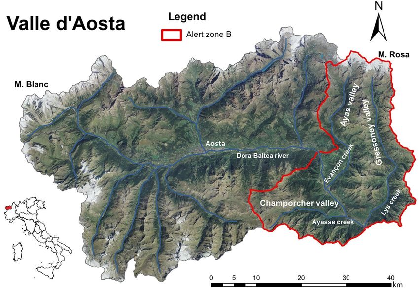
1920          T. Salvatici et al.: Application of a physically based model to forecast shallow landslides at a regional scale

racy, producing accurate hazard maps that can be of help for       and the erosive depositional forms found in the Ayas Valley.
landslide risk assessment and management.                          The three valleys’ watercourses, the Lys Creek, the Evançon
   In this work, we apply the physically based HIRESSS             Creek, and the Dora Baltea River, contributed to the glacial
(HIgh REsolution Slope Stability Simulator) model (Rossi           deposits modeling with the formation of alluvial fans. The
et al., 2013) in the eastern section of the Aosta Valley region    climate of the region is characterized by high variability that
(Italy), in the northwest Alpine mountain chain, in order to       is strongly influenced by altitude (ranging from 400 m a.s.l.
test the capacity of the model to forecast the occurrence of       of Dora Baltea River’s floodplain to 4810 m a.s.l. of Mont
shallow landslides at the regional scale. In particular, the ob-   Blanc), with a continental climate in the valley floors and an
jectives of this study are as follows: (i) to properly charac-     Alpine climate at high altitudes.
terize the geotechnical and hydrological parameters of the            The slope steepness and the mean annual precipitation of
soil to feed the HIRESSS model, and to spatialize this punc-       800–900 mm are the main landslide triggering factors. These
tual information in order to have spatially continuous maps        features lead the study area to be prone to landsliding, in
of the model input data; and (ii) to test the HIRESSS code for     particular rockfalls, deep seated gravitational slope defor-
two selected rainfall events, which triggered several shallow      mations (DSGSD), rocks avalanches, debris avalanches, de-
landslides, and to validate the model results. HIRESSS is a        bris flows, and debris slides (Catasto dei Dissesti Regionale
physically based distributed slope stability simulator for an-     – form Val d’Aosta Regional Authorities). In this work we
alyzing shallow landslide triggering conditions in real time       model the triggering conditions of shallow landslides, i.e.,
and over large areas using parallel computational techniques.      soil slips and translational slides, and we do not take other
In the area selected, an in-depth study of the geotechnical        types of movement into account.
and hydrological properties of hillslopes controlling shallow         The HIRESSS model simulated two past events, one in
landslides formation was conducted; this involved perform-         2008 and one in 2009, and a validation of the model perfor-
ing two campaigns (using 12 survey points) of in situ mea-         mance was then carried out comparing the results with the
surements and laboratory tests. Furthermore, the HIRESSS           landslide regional database.
model was modified to take the effect of the root reinforce-          The two simulated events are as follows:
ment to the stability of slopes based on plant species distri-
bution and literature values of root cohesion into account.            – 24–31 May 2008: on 28 and 29 May 2008 intense and
                                                                         persistent rainfall was recorded across the Aosta Val-
                                                                         ley region with a total precipitation in the study area of
2   Study area and rainfall events                                       about 250 mm causing flooding, debris flows, and rock-
                                                                         falls.
The study area, called “alert zone B” by the regional civil
protection authorities, is located in the eastern part of the          – 25–28 April 2009: from 26 to 28 April 2009 heavy rain-
Aosta Valley region, in the northwest Alpine mountain chain              fall affected the southeastern part of the Aosta Valley
(Fig. 1). The area is characterized by three main valleys:               region, with the highest precipitation of about 268 mm
Champorcher Valley, Gressoney or Lys Valley, and Ayas Val-               recorded at the Lillianes Granges station. This precipi-
ley. The first is located on the right side of the Dora Bal-             tation triggered several landslides.
tea catchment, and represents the southern part of the study
area. The second and third valleys show a north–south orien-       3     Methodology
tation, and are delimited to the north by Monte Rosa Massif
(4527 m a.s.l.) and to south by the Dora Baltea River.             3.1    HIRESSS description
   From a geological point of view, the Aosta Valley is lo-
cated northwest of the Insubric Line; in particular, there are     The physically based distributed slope stability simulator
three systems of Europa chain: the Austroalpine, the Pen-          HIRESSS (Rossi et al., 2013) is a model developed to an-
ninic and the Helvetic systems (De Giusti, 2004). Figure 2         alyze shallow landslide triggering conditions on a large scale
shows the lithological map of the study area obtained by           at high spatial and temporal resolutions using a parallel cal-
reclassifying the geological units according to 11 litholog-       culation method. The model is composed of a hydrological
ical groups: landslides, calcareous schist, alluvial deposits,     and a geotechnical component (Rossi et al., 2013). The hy-
glacial deposits, colluvial deposits, glacier, granites, mica      drological component is based on dynamic input of the rain-
schists, green stone, black schists, and serpentinites. The        fall data, which are used to calculate the pressure head and
main lithologies outcropping in the study area are metamor-        provide it to the geotechnical stability model. The hydrolog-
phic and intrusive rocks, in particular granites, metagranites,    ical model is initiated as a modeled form of hydraulic dif-
schists, and serpentinite.                                         fusivity using an analytical solution, which is an approxi-
   The geomorphology of the region is characterized by steep       mated form of the Richards equation under the wet condition
slopes and valleys shaped by glaciers. The glacial model-          (Richards, 1931). The equation solution allows us to calcu-
ing is shown in the U-shape of the Lys and Ayas valleys,           late the pressure head variation (h), depending on time (t)

Nat. Hazards Earth Syst. Sci., 18, 1919–1935, 2018                          www.nat-hazards-earth-syst-sci.net/18/1919/2018/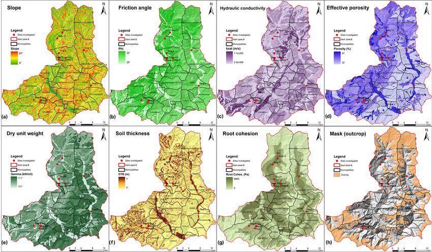
T. Salvatici et al.: Application of a physically based model to forecast shallow landslides at a regional scale                       1921

Figure 1. The Aosta Valley region in northwest Italy. The study area, alert zone B, is delineated in red.

and the depth of the soil (Z). The solutions are obtained by              area ratio (proportion of area occupied by roots per unit area
imposing some boundary conditions as described by Rossi et                of soil), k is a coefficient dependent on the effective soil fric-
al. (2013).                                                               tion angle and the orientation of roots. The measure of cr
   The geotechnical stability model is based on an infinite               varies with vegetal species; within a single species the mea-
slope stability model. The model considers the effect of                  sure depends on how plants respond to environmental char-
matric suction in unsaturated soils, taking the increase in               acteristics and fluctuations.
strength and cohesion into account. The stability of the slope               Therefore, the new equation for FS at unsaturated condi-
at different depths (Z values) is computed, as the hydrolog-              tions is as follows:
ical model calculates the pressure head at different depths.                     tan ϕ      ctot
The variation of soil mass caused by water infiltration on par-           FS =          +
                                                                                 tan α γd y sin α
tially saturated soil is also modeled. The original FS (factor                             (                  λ )−1
of safety) equations (Rossi et al., 2013) were modified tak-
                                                                                                   −1
                                                                                                       λ+1  λ+1
ing the effect of root reinforcement (cr ) as an increase of soil                γw h tan ϕ 1 + hb |h|
cohesion (c0 ) into account as follows:                                      +                                             ,            (3)
                                                                                                  γd y sin α
ctot = c0 + cr .                                                 (1)      where φ is the friction angle, α is the slope angle, γd is the dry
                                                                          soil unit weight, y is the depth, γw is the water unit weight,
   Regarding the geotechnical influence of roots on the soil              h is the pressure head, hb is the bubbling pressure, and λ
strength, roots seem to affect the cohesion parameter only,               is the pore size index distribution. In saturated condition the
while the friction angle is poorly or not at all impacted                 equation for FS (Rossi et al., 2013) becomes
by reinforcement (Waldron and Dakessian, 1981; Gray and
Ohashi, 1983; Operstein and Frydaman, 2000; Giadrossich                        tan ϕ                ctot
                                                                          FS =       +
et al., 2010). Therefore, it is necessary to consider the root                 tan α (γd (y − h) + γsat h) sin α
cohesion when calculating the FS and consequently when ap-                             γw h tan ϕ
plying the HIRESSS model.                                                    −                             ,                            (4)
                                                                               (γd (y − h) + γsat h) tan α
   The root reinforcement (or root cohesion) can be consid-
ered equal to (Eq. 2):                                                    where γsat is the saturated soil unit weight.
                                                                             One of the major problems, associated with the determin-
cr = kTr (Ar A) ,                                                (2)      istic approach employed on a large scale, is the uncertainty
                                                                          of the static input parameters or geotechnical parameters of
where Tr is the root failure strength (tensile, frictional, or            the soil. The method used for the estimation of parameters’
compressive) of roots per unit area of soil, Ar /A is the root            spatial variability is the Monte Carlo simulation. The Monte

www.nat-hazards-earth-syst-sci.net/18/1919/2018/                                  Nat. Hazards Earth Syst. Sci., 18, 1919–1935, 2018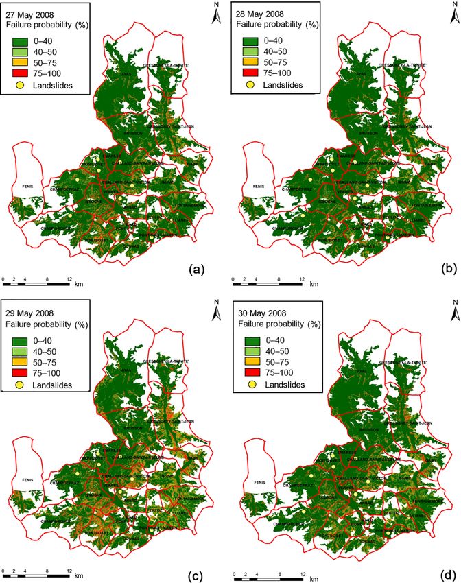
1922           T. Salvatici et al.: Application of a physically based model to forecast shallow landslides at a regional scale

Figure 2. Spatial distribution of survey points compared to the geolithology.

Carlo simulation achieves a probability distribution of input            3.2    HIRESSS input data preparation
parameters, providing results in terms of slope failure prob-
ability (Rossi et al., 2013). The developed software uses the            The input parameters can be divided in two classes: the static
computational power offered by multicore and multiproces-                data and the dynamical data. Static data are geotechnical and
sor hardware, from modern workstations to supercomput-                   morphological parameters while dynamical data are repre-
ing facilities (HPC), to achieve the simulation in a reason-             sented by the hourly rainfall intensity. Static data are read
able runtime and is compatible with civil protection real-               only once at the beginning of the simulation while dynami-
time monitoring (Rossi et al., 2013). The HIRESSS model                  cal inputs are continuously updated.
loads spatially distributed data arranged as 12 input raster                The HIRESSS input is in raster, which means that point
maps and the maps of rainfall intensity. These input raster              data and parameters have to be adequately spatially dis-
maps are slope gradient, effective cohesion (c0 ), root cohe-            tributed. In this application the spatial resolution was 10 m.
sion (cr ), friction angle (φ 0 ), dry unit weight (γd ), soil thick-
ness, hydraulic conductivity (ks ), initial soil saturation (S),         Static data
pore size index (λ), bubbling pressure (hb ), effective poros-
ity (n), residual water content (qr ), and rainfall intensity.           The slope gradient was calculated from the DEM (digital
                                                                         elevation model). The DEM has a resolution of 10 m and
                                                                         is dated 2006. Effective cohesion, friction angle, hydraulic
                                                                         conductivity, effective porosity, and dry unit weight were ob-
                                                                         tained and spatialized according to lithology. The soil punc-

Nat. Hazards Earth Syst. Sci., 18, 1919–1935, 2018                               www.nat-hazards-earth-syst-sci.net/18/1919/2018/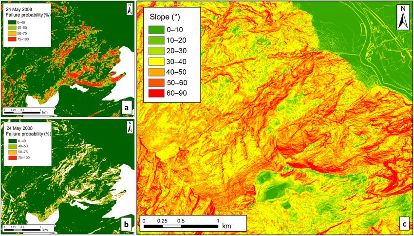
T. Salvatici et al.: Application of a physically based model to forecast shallow landslides at a regional scale              1923

tual parameters were derived from the in situ and laboratory         – direct shear test on selected samples.
geotechnical tests and analysis.
   In particular, the properties of slope deposits were deter-
mined by in situ and laboratory measurements (Bicocchi et             Soil thickness was calculated by the GIST model (Catani
al., 2016; Tofani et al., 2017) at 12 survey points. To carry      et al., 2010; Del Soldato et al., 2016). Soil characteristic
out the in situ tests the survey points were selected using the    curves parameters (pore size index, bubbling pressure, and
following characteristics: (i) physiography, (ii) landslides oc-   residual water content) were derived from literature values
currence, and (iii) geolithology (Fig. 2). Regarding the first     (Rawls et al., 1982).
point, a high-resolution DEM (from Val d’Aosta Regional               Root cohesion variations in the area (at the soil depth cho-
Authorities) and careful first surveys were used to identify       sen for the physical modeling with HIRESSS) were first ob-
the most suitable slopes. The surveys took place in two ses-       tained, identifying the plant species and determining their
sions, the first in August 2016, and the second in Septem-         distribution from in situ observations and vegetational maps
ber 2016. The following analyses were conducted:                   (Carta delle serie di vegetazione d’Italia, Italian Ministry of
                                                                   the Environment and Protection of Land and Sea). Then,
  – Registration of the geographical position was under-           the measure of cohesion due to the presence of roots was
    taken using a GPS and photographic documentation of            assigned to each subarea according to the dominant plant
    the site characteristics (morphology and vegetation).          species and literature root cohesion value for that species
  – The in situ measurement of the saturated hydraulic con-        (Bischetti, 2009; Burylo et al., 2010; Vergani et al., 2013,
    ductivity (ks ) was carried out by means of the constant       2017), which were calculated considering the fiber bundle
    head well permeameter method using an Amoozemeter.             model (Pollen et al., 2004). The measure of cr varies with
                                                                   vegetal species; within a single species the value depends
  – Sampling of an aliquot (∼ 2 kg each) of the material was       on how plants respond to environmental characteristics and
    conducted for laboratory tests, including grain size dis-      fluctuations. Therefore, a map of root cohesion variations,
    tributions, index properties, Atterberg limits, and direct     obtained as previously mentioned, is a simplification of real-
    shear tests.                                                   ity. This is a necessary simplification as the known methods
                                                                   to evaluate root cohesion variations are not suitable for wide
   The permeability in situ measurements and the soil sam-
                                                                   areas and acceptable measurement times.
plings were made at depths ranging from 0.4 to 0.6 m below
                                                                      The last static input data, in this study, are the exposure
the ground level. The evaluation of the ks (saturated hydraulic
                                                                   rock mask. These data were defined considering the litholog-
conductivity or permeability) was made with an Amoozeme-
                                                                   ical and land use maps, so that the HIRESSS model avoided
ter permeameter (Amoozegar, 1989). The measurement was
                                                                   simulation on steep slopes made of bare rocks.
obtained by observing the amount of water required to main-
                                                                      The geotechnical properties and root cohesion of the soils
tain a constant volume of water in the hole. In situ measure-
                                                                   have been spatialized with respect to a lithological classifica-
ments were then entered into the Glover solution (Amooze-
                                                                   tion.
gar, 1989), which calculated the saturated permeability of the
                                                                      For each lithological class and plant species the mean
soils. The ks is a very useful parameter not only for slope sta-
                                                                   value has been selected in order to obtain the HIRESSS input
bility modeling but also for many other hydrological prob-
                                                                   raster parameters.
lems (groundwater, surface water and sub-surface runoff, and
flow calculation of water courses).
   In addition, the samples collected in situ were examined in     Dynamic data
the laboratory to define a wide range of parameters to more
extensively characterize the deposits. In particular, the fol-     In the study area, the rainfall hourly data from 27 pluviome-
lowing tests were performed in order to classify the analyzed      ters were available; therefore, it was necessary to spatially
soils:                                                             distribute them to generate a 10 × 10 m cell size input raster
                                                                   to ensure correct program operation. The rainfall data were
  – grain size distribution (determination of granulometric        elaborated by applying the Thiessen polygon methodology
    curve for sieving and settling following ASTM recom-           (Rhynsburger, 1973), modified to take the elevation into ac-
    mendations), and classification of soils (according to         count. Thiessen polygon methodology allows us to divide a
    AGI and USCS classification, Wagner, 1957);                    planar space into regions, and to assign the regions to the
                                                                   nearest point feature. This approach defines an area around
  – determination of the main index properties (porosity, re-
                                                                   a point, where every location is nearer to this point than to
    lationships of phases, natural water content (wn ), the re-
                                                                   all the others. Thiessen polygon methodology does not con-
    spective natural and dry unit weight (γ ) and (γd )) fol-
                                                                   sider the morphology of the area; therefore, alert zone B was
    lowing the ASTM recommendations;
                                                                   divided in three catchment areas and the polygons were cal-
  – determination of Atterberg limits (liquid limit (LL),          culated for each of the rain gauges considering the reference
    plastic limit (PL), and plasticity index (PI));                catchment basin (Fig. 3).

www.nat-hazards-earth-syst-sci.net/18/1919/2018/                          Nat. Hazards Earth Syst. Sci., 18, 1919–1935, 2018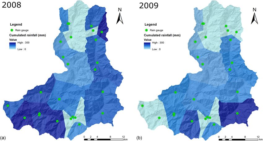
1924            T. Salvatici et al.: Application of a physically based model to forecast shallow landslides at a regional scale

Figure 3. Comparison of Thiessen polygons methodology; (a) simple and (b) modified according to the catchment basins boundaries.

4     Results                                                        10−6 m s−1 . The minimum and maximum values were found
                                                                     between 1.36 · 10−7 and 1.54 · 10−5 m s−1 . Considering the
4.1    HIRESSS input data                                            poor variability of samples, the permeability values were rel-
                                                                     atively homogeneous and in accordance with the values re-
The results of the geotechnical and hydrological characteri-         ported in the literature (Table 1).
zation of the soils of the 12 survey points are shown in Ta-            The additional cohesion induced by roots assumes differ-
ble 1 for all survey sites.                                          ent values not only depending on plant species and envi-
   The results of granulometric tests show that the analyzed         ronmental characteristics but also on depth of soil, as roots’
soils are predominantly sands with silty gravel (Fig. 4 and          diameter and density vary with latter. Because of such ev-
Table 1). Regarding the index properties, the natural soil wa-       idence, studies on root cohesion in different species report
ter content values were predominantly about 20 % by weight,          values as a function of soil depth. In this study region, soils
with maximum and minimum values of 5.1 and 26.2 %, re-               were thinner than in areas where previous studies have been
spectively. These values reflect their different ability to hold     carried out. In such thin soils, root systems organize their
water in their voids. The measured natural unit weight (γ )          growth depending on available space and do not reach the
varied between 15.3 and 21.7 kN m−3 , depending not only             same depth as roots in thick soils. Consequently, in this con-
on the different grain size distribution but also on the dif-        text root cohesion of species at different depths was dissim-
ferent thickening and consolidation states. In addition, the         ilar to the literature values. Considering this, the map re-
measured values for the saturated unit weight (γsat ) ranged         garding the variation of root cohesion was processed taking
between 18.2 and 21.5 kN m−3 (Table 1).                              the minimum cohesion value for each species (among those
   The Atterberg limits (LL and PL) were measured on sam-            specified for each species at the different depth) reported in
ples with a sufficient passing fraction (> 30 % by weight)           literature. By doing this, the contribution of vegetation to the
through a 40 ASTM (0.425 mm) sieve. For prevalently sandy            stability of slopes is considered in the FS calculation, whilst
samples, LL values were mostly around 40 % of water con-             an overestimate of root cohesion is avoided.
tent (% by weight), while the PL was around 30 % (Table 1).             In the study area, root cohesion, defined as mentioned
   The effective friction angle varied between a minimum of          above, ranged from a minimum of 0.0 kPa (mainly in the
25.6 and a maximum of 34.3◦ , while the effective cohesion           outcrop area) to a maximum of 8.9 kPa (in areas occupied
ranged from a minimum of 0.0 to a maximum of 9.3 kPa.                by mountain maple on the left bank of Dora Baltea River).
Consistent with the presence of sandy soils, the saturated              In Table 2, the mean values of each of the input parameters
permeability values were around a medium-high value of               are reported with respect to lithological class.

Nat. Hazards Earth Syst. Sci., 18, 1919–1935, 2018                           www.nat-hazards-earth-syst-sci.net/18/1919/2018/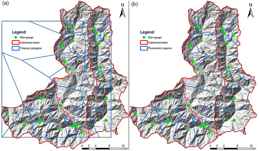
Table 1. Geotechnical properties of survey points (grain size distribution, Atterberg limits, index properties, permeability, and shear strength parameters).

                                                      Site      Soil type          G       S      M       C     LL      PL       PI     USCS       γ          γd          γsat      n       w          ks            ksc       φ 0 lab     c’
                                                                                   %       %      %       %     (%)     (%)     (%)            (kN m−3 )   (kN m−3 )   (kN m−3 )   (%)     (%)       (m s−1 )      (m s−1 )      (◦ )    (kPa)
                                                      Site 1    Sand with         27.8    45.2    23.4   3.6     36      25      11     SM       16.7        13.7        18.3      47.3    11.3         /        2.52 × 10⁻⁶   25.6       1.0
                                                                silty gravel
                                                      Site 2    Sand with         19.4    50.5    29.0   1.1     38      25      14      SC      19.1        14.5        18.8      44.3    11.4    2.71 × 10⁻⁶   1.48 × 10⁻⁶   34.3       1.5
                                                                gravelly silt
                                                      Site 3    Sand with         26.9    45.2    26.8   1.1      /       /       /      /         /           /           /         /       /          /        8.89 × 10⁻⁷      /        /
                                                                gravel and silt
                                                      Site 4    Sand with         18.8    40.4    39.2   1.6     38      27      11     SM       19.5        14.8        19.0      43.2    10.7    1.36 × 10⁻⁷   4.51 × 10⁻⁷   34.3       0.0
                                                                gravelly silt
                                                      Site 5    Sand with         31.0    43.1    25.7   0.2     47      36      11     SM       18.4        14.0        18.5      46.3    11.0         /        2.44 × 10⁻⁶   25.7       9.3

www.nat-hazards-earth-syst-sci.net/18/1919/2018/
                                                                gravel and silt
                                                      Site 6    Sand with         28.5    57.5    13.9   0.1     52      38      13     SM       18.7        13.5        18.2      47.9    20.0         /        8.27 × 10⁻⁶   30.2       4.4
                                                                poorly
                                                                silty gravel
                                                      Site 7    Sand with         37.0    42.6    17.9   2.5     40      32      8      SM       20.3        15.5        19.5      40.4    26.2    5.18 × 10⁻⁶   2.97 × 10⁻⁶   28.2       3.4
                                                                silty gravel
                                                      Site 8    Sandy silty       58.1    24.6    16.0   1.3     43      28      16     GM       17.2        15.7        19.6      39.6     9.4         /        3.76 × 10⁻⁶   30.1       8.1
                                                                gravel
                                                      Site 9    Gravelly          18.7    55.1    24.4   1.8     46      36      10     SM       20.1        18.7        21.5      27.9     8.1    2.41 × 10⁻⁶   1.73 × 10⁻⁶   33.9       0.6
                                                                silty sand
                                                      Site 10   Sand with         21.9    52.0    25.1    1      46      37      8      SM       18.4        16.0        19.8      38.6    15.5         /        2.10 × 10⁻⁶   30.3       1.5
                                                                gravelly silt
                                                      Site 11   Gravelly          24.3    51.4    21.2   3.1     31      25      7      SM       21.7        18.0        21.2      31.9    20.5    4.03 × 10⁻⁶   3.05 × 10⁻⁶   29.8       2.0
                                                                silty sand
                                                      Site 12   Gravel with       55.2    32.2    12.2   0.4     55      45      10     SM       15.3        14.6        18.9      43.9     5.1    1.54 × 10⁻⁵   8.25 × 10⁻⁶   30.2       1.6
                                                                poorly
                                                                silty sand
                                                                Mean              30.63   44.98   22.9   1.48   42.91   32.18   10.82           18.67       15.36       19.39      41.03   13.56   4.98 × 10⁻⁶   3.16 × 10⁻⁶   30.24     3.04
                                                                Median            27.35    45.2   23.9    1.2    43      32      11              18.7        14.8        19.0       43.2    11.3   3.37 × 10⁻⁶   2.48 × 10⁻⁶    30.2      1.6
                                                                SD                13.31   9.48    7.41   1.11   7.15    6.71    2.71            1.80        1.68        1.10       6.34    6.30    5.38 × 10⁻⁶   2.56 × 10⁻⁶    3.05     3.07
                                                                Max                58.1   57.5    39.2   3.6     55      45      16              21.7        18.7        21.5      47.9     26.2   1.54 × 10⁻⁵   8.27 × 10⁻⁶    34.3      9.3
                                                                Min               18.7    24.6    12.2   0.1     31      25       7             15.3        13.5        18.2       27.9     5.1    1.36 × 10⁻⁷   4.51 × 10⁻⁷    25.6       0
                                                                                                                                                                                                                                                 T. Salvatici et al.: Application of a physically based model to forecast shallow landslides at a regional scale

Nat. Hazards Earth Syst. Sci., 18, 1919–1935, 2018
                                                                                                                                                                                                                                                 1925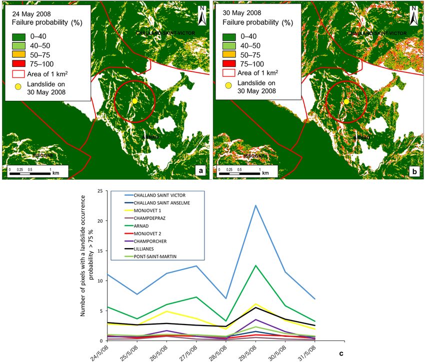
1926           T. Salvatici et al.: Application of a physically based model to forecast shallow landslides at a regional scale

Figure 4. Grain size distributions of soil samples (F is fine, M is medium and C is coarse).

Table 2. Spatialized geotechnical parameters of each lithological class as input for the HIRESSS model.

               Lithological    Soil type       φ’ lab     c’         γd          n        ks          hb       qr      λ
               classes                          (◦ )     (Pa)     (kN m−3 )     (%)     (m s−1 )
               Calcareous      Sand with         31      1000       16.5        39    1.1 × 10⁻⁵    0.1466   0.041   0.322
               schist          gravelly silt
               Alluvial        Sand with         26      1000       14.0        46    3.0 × 10⁻⁶    0.1466   0.041   0.322
               deposits        gravel and
                               silt
               Glacial         Sand with         31      1000       15.3        41    2.7 × 10⁻⁶    0.1466   0.041   0.322
               deposits        silty gravel
               Colluvial       Sand with         25      1000       13.7        47    2.5 × 10⁻⁶    0.1466   0.041   0.322
               deposits        silty gravel
               Granites        Sandy gravel      30      1000       17.6        32    4.0 × 10⁻⁶    0.1466   0.041   0.322
               Mica            Sandy             30      1000       17.7        32    6.0 × 10⁻⁶    0.1466   0.041   0.322
               schists         silty gravel
               Green           Gravel with       32      1000       16.3        37    4.6 × 10⁻⁶    0.1466   0.041   0.322
               stones          silty sand

   The pore size index, bubbling pressure, and residual water              probability. The main characteristics of the simulation are
content were constant in the study area, measuring 0.322 (−),              shown in Table 3.
0.1466 m, and 0.041 (−), respectively.                                        The results of the simulations for both events on the first
   The distributed soil parameter maps are shown in Fig. 5.                day of the simulation showed pixels with a high landslide
The results of rainfall data, elaborated using Thiessen poly-              probability occurrence in absence of rainfall. These pixels
gon methodology, are 192 and 96 rainfall hourly maps for the               were false positives (i.e., pixels identified unstable by the
2008 and 2009 events, respectively. In Fig. 6 the cumulative               model but were not really unstable) and occurred due to mor-
maps of each event are shown.                                              phometric reasons, predominantly high slope angles. To re-
                                                                           move these false positives, a numeric mask was applied. Us-
4.2    HIRESSS simulation                                                  ing GIS software commands, it was possible to calculate the
                                                                           number of pixels on the first simulation day with a trigger
The HIRESSS model was used to simulate two past events;                    probability value greater than 80 % and delete them (Fig. 7).
one in 2008 (24–31 May) and one in 2009 (25–28 April),                     The mask was then applied to the rest of landslide occur-
both of which triggered several landslides in the study area.              rence probability maps. The resulting maps for each days of
  The HIRESSS input data were entered into the HIRESSS                     the simulated events are shown in the Figs. 8 and 9.
model to obtain day-by-day maps of the landslide occurrence

Nat. Hazards Earth Syst. Sci., 18, 1919–1935, 2018                                www.nat-hazards-earth-syst-sci.net/18/1919/2018/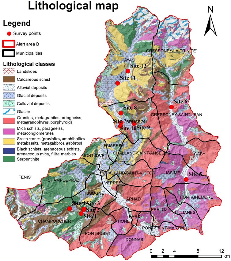
T. Salvatici et al.: Application of a physically based model to forecast shallow landslides at a regional scale                           1927

Figure 5. Static input parameters for HIRESSS model: (a) slope gradient, (b) friction angle, (c) hydraulic conductivity, (d) effective porosity,
(e) dry unit weight, (f) soil thickness, (g) root cohesion, and (h) exposure rock mask.

Figure 6. Cumulated rainfall maps for the two events.

www.nat-hazards-earth-syst-sci.net/18/1919/2018/                                  Nat. Hazards Earth Syst. Sci., 18, 1919–1935, 2018
1928 T. Salvatici et al.: Application of a physically based model to forecast shallow landslides at a regional scale
Figure 7. Example of the numerical mask used to remove the false positives for the first event simulated (24–31 May 2008). (a) The HIRESSS
result for the first day of simulation with false positive pixels. (b) The probability map after the numerical mask implementation. (c) The
slope map, which shows that the pixels with high probability of landslide occurrence are located where the slope is higher than 60 %.
Table 3. Main characteristics of the simulation. of the region where the cumulated rainfall average was about
151 mm. The probability maps show high values during these
2008 2009 days (Fig. 9c, d). This event led to many landslides being
event event triggered (as reported in the database).
Spatial resolution 10 m 10 m In order to validate the HIRESSS simulations the database
Time step 1h 1h of landslides triggered during the two events were compared
Rainfall ( h) 192 96 with the models results.
In general, for both events temporal validation showed
that the daily highest probability of occurrence, computed by
HIRESSS, correspond with days with landslide occurrences
The results of the first simulated event (24–31 May 2008) and the most intense precipitation.
are shown in Fig. 8. The failure probability in the whole For the first simulated event, landslides reported in the
area was negligible for the first four days (from 24 to database are dated 30 and 31 May 2008 (Fig. 8d) which cor-
27 May 2008) (Fig. 8a). The rainfall intensity then increased respond to the days with highest probability of occurrence.
from 27 May and reached its highest value on 29 May, when The same can be seen for the second event, with many land-
the precipitation value was around 100 mm in the eastern sec- slides being triggered between 27 and 28 April 2009 (as re-
tor of study area. The HIRESSS model simulate this pas- ported in the database).
sage well, with the 28 and 29 May 2008 landslide occur- In Table 4 the results with over a 75 % slope failure proba-
rence probability maps showing a considerable increase in bility for both events are highlighted and confirm the correct
the probability of failure with maximum values around 90 % temporal occurrence of landslides. In particular, we notice
in the east of alert zone B (Fig. 8b, c). In the following days that for the first event (2008) the number of unstable pix-
rainfall intensity decreases, and the probability also slowly els (failure probability > 75 %) increases from 29 May with
decreases, although it is still high on 30 May 2008. a total extension of the unstable area of about 24 km2 . For
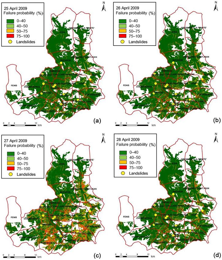
Concerning the second event (25–28 April 2009), the land- the 2009 event, the number of unstable pixels increases from
slide occurrence probability was negligible for the first two 27 April with an extension of 33 km2 .
days (25 and 26 April 2009) over the whole area (Fig. 9a, b), Temporal validation was also carried out, considering
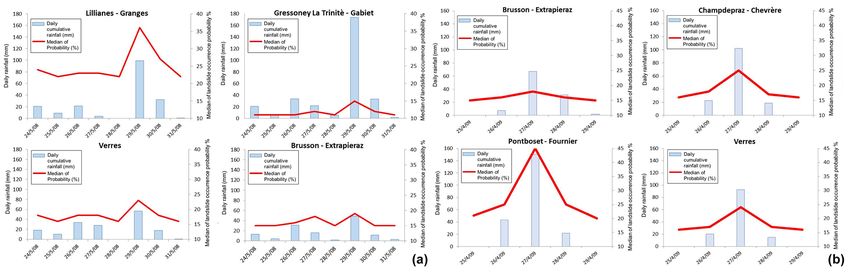
due to the low rainfall intensity. From 27 April 2009 rain- daily cumulative rainfall compared to the landslide failure
fall became more intense, especially in the southeast sector
Nat. Hazards Earth Syst. Sci., 18, 1919–1935, 2018 www.nat-hazards-earth-syst-sci.net/18/1919/2018/T. Salvatici et al.: Application of a physically based model to forecast shallow landslides at a regional scale 1929 Figure 8. HIRESSS landslide probability maps of the simulated event from 24 to 31 May 2008 and the reported landslides during this event, with on the four critical days: (a) 27 May 2008, (b) 28 May 2008, (c) 29 May 2008, and (d) 30 May 2008. probability. In particular, a median of the landslide occur- the reports of landslide events may have errors regarding the rence probability was calculated for four pluviometric areas precise spatial location and the size of the phenomenon. To identified by Thiessen polygons methodology, modified ac- overcome this problem and to take probable errors caused by cording to limits of river basins; this was undertaken both the actual spatial location in the database into account, an for the event in May 2008 and for the event in April 2009 area of 1 km2 (called the influence area) around the point of (Fig. 10a, b). As could be expected, the results showed that the landslide was considered in the validation analysis. In- when the highest rainfall intensity was measured, the highest side the influence area, pixels that had a 75 % probability of probability of occurrence was computed for all areas and for failure were considered unstable. both events. Figure 11 shows an example of a landslide event that oc- Spatial validation was performed following a pixel-by- curred in the Arnad municipality on 30 May 2008. The model pixel method, which is the most complex method and con- computes a low failure probability on 24 May 2008 and an in- sists of comparing the probability of the instability of each crease in the failure probability on 30 May 2008. In Fig. 11a pixel with the pixels involved in the actual event. This vali- and b it is possible to note that, inside the red circle, the dation implies a great deal of uncertainty in the results, since red and yellow areas have increased on 30 May with re- www.nat-hazards-earth-syst-sci.net/18/1919/2018/ Nat. Hazards Earth Syst. Sci., 18, 1919–1935, 2018
1930          T. Salvatici et al.: Application of a physically based model to forecast shallow landslides at a regional scale

Figure 9. HIRESSS landslide probability maps of the simulated event between 25 and 28 April 2009 and the reported landslides during this
event, (a) 25 April 2009, (b) 26 April 2009, (c) 27 April 2009, and (d) 28 April 2009.

Figure 10. Correlation graphs between the daily cumulative rainfall and the median of the landslide occurrence probability for both events.

Nat. Hazards Earth Syst. Sci., 18, 1919–1935, 2018                               www.nat-hazards-earth-syst-sci.net/18/1919/2018/
T. Salvatici et al.: Application of a physically based model to forecast shallow landslides at a regional scale                  1931

Table 4. HIRESSS results for both the 2008 and 2009 events.             Validation of the model results
“No. pixel” represents the number of pixels with a slope failure
probability over 75 %; “Total %” represents the percentage of pix-      To perform a solid validation it is necessary to have informa-
els with slope failure probability over 75 %; and “Pixel area (km2 )”   tion regarding the spatial location and temporal occurrence
represents the extension of the area with slope failure probability     of landslides. In particular, the time of occurrence is very
over 75 %.                                                              rarely known with hourly precision; this is due to the fact
                                                                        that landslides are usually related to a rainstorm, without any
            2008 event       No. pixel    Total    Pixel
                                                                        other precise information on time of occurrence (Rossi et al.,
                                             %      area
                                                  (km2 )
                                                                        2013). Concerning the spatial landslides locations, in many
                                                                        cases they are only included in the database as points with-
            24 May 2008        62 344         1        6                out any information on the area involved. In our database,
            25 May 2008        21 295         0        2                provided by the local authorities, landslides are points with
            26 May 2008        84 256         1        8                information on the day of occurrence.
            27 May 2008        95 220         1       10
                                                                           In synthesis the main problems encountered during the
            28 May 2008        15 364         0        2
            29 May 2008       243 137         3       24
                                                                        model validation are as follows:
            30 May 2008        79 437         1        8
            31 May 2008         7110          0        1                  – The incompleteness of landslide datasets. In general
                                                                            event-based databases are incomplete due to a lack
            2009 event       No. pixel    Total    Pixel
                                                                            of reporting in mountainous, scarcely populated areas,
                                             %      area
                                                                            while most of reported landslides involve infrastructure
                                                  (km2 )
                                                                            or water streams (Mercogliano et al., 2013, Tofani et al.,
            25 Apr 2009             0         0        0                    2017). In our case we have two datasets for the two sim-
            26 Apr 2009        52 644         1        5                    ulated events (2008 and 2009) with 9 and 11 landslides,
            27 Apr 2009       326 826         4       33                    respectively. The number of reported landslides is very
            28 Apr 2009        56 599         1        6                    low and not suitable to perform a correct validation for
                                                                            the whole area. In fact, in both events there are some
                                                                            areas that show a high failure probability even though
spect to 24 May. In this case, the model was able to correctly              there are no landslides reported. For example, for the
identify such movement. To better highlight this validation,                2008 event (Fig. 8), the municipalities of Gressoney
Fig. 11c shows the number of pixels above 75 % probability                  Saint Jean and Gaby in the northeast portion of the study
that were calculated by the model within a ca. 1 km2 circu-                 area and the municipalities of Pontboset and Issogne
lar area around all the landslides that occurred during 2008                in the southern part of the study area show high fail-
event. For some of the reported landslide events, the number                ure probabilities (> 75 %) but no reported landslides.
of pixels above 75 % increases on 30 May 2008; however,                     The same occurs for the 2009 event (Fig. 9) when Gres-
in the cases of the Champdepraz and Montjovet 2 events the                  soney Saint Jean and Pontboset as well as Lillianes and
probability does not increase. This may have been caused by                 Fontainemore in the southeast portion of the study area
the low precision regarding the location of the reported land-              show high failure probabilities but no recorded land-
slide, and because some of the real landslides reported are                 slides. In these cases, we are not able to discriminate if
other types of movements (rockfalls, rotational slides) that                the model has overestimated the landslide occurrence or
cannot simulated by the HIRESSS model.                                      it has correctly predicted landslide occurrence since we
                                                                            are not certain about the completeness of the database.

5   Discussion                                                            – Correct spatial location. In our validation landslide
                                                                            dataset the accuracy of the spatial location was very
The application of the HIRESSS model to a portion of the                    low and the landslides were reported as points (yellow
Aosta Valley region provided good results in terms of the                   dots in Figs. 8 and 9). Furthermore, we did not know for
spatial and temporal accuracy of the model as highlighted                   certain if these points correspond to the triggering area
in Sect. 4.2. The advantage of the regional physically based                (which would constitute the desirable situation), to the
model, with respect to rainfall thresholds, is that it is possible          deposition area, or to the position of the elements at risk
to predict the occurrence of shallow landslides with metric                 (house, road, river) from the landslides. For this reason,
spatial resolution and hourly temporal resolution.                          when performing the spatial validation, we considered
   Conversely, the application of the HIRESSS model has                     an area of 1 km2 around the point in order to take the
highlighted some important drawbacks, mainly related to (i)                 error in the spatial location of the landslides into ac-
the validation of the models results and (ii) the uncertainty of            count (Fig. 11). In these cases, where the position of the
the input parameters.                                                       landslides were uncertain, an alternative solution could

www.nat-hazards-earth-syst-sci.net/18/1919/2018/                               Nat. Hazards Earth Syst. Sci., 18, 1919–1935, 2018
1932 T. Salvatici et al.: Application of a physically based model to forecast shallow landslides at a regional scale
Figure 11. An example of a landslide event that occurred in the Arnad municipality compared to a landslide occurrence probability map,
(a) before and (b) after a rainfall event. (c) The number of pixels above 75 % failure probability calculated by the model for all the landslides
triggered during the event in the study area.
be to perform a validation aggregating the results us- analysis of the model performance could only have been
ing different spatial units, such as first or second order carried out if information on the exact time of failure
basins as proposed in Rossi et al. (2013). Whilst spatial was available.
aggregation overcomes the problem of establishing the
correct location of landslides for validation, it causes the Uncertainty of the input parameters
high spatial resolution of the HIRESSS model to be lost,
which is one of the major benefits of the analysis . The Another important limitation related to the application and
ideal situation would be to have a landslide database re- accuracy of the physically based model is the availability
alized with the same resolution as the HIRESSS model. of detailed databases of the physical and mechanical prop-
erties of soils in the study areas. The performance of a model
– Temporal occurrence. The event landslide database pro- can be strongly influenced by the errors or uncertainties in
vides information concerning the day of the landslide such input data (Segoni et al., 2009; Jiang et al., 2013).
occurrence. The HIRESSS model has a higher temporal Furthermore, the punctual information regarding soil prop-
resolution, as it is able to provide hourly failure proba- erties has to be spatialized and, in general, is characterized
bility maps (Table 3). In order to make a temporal val- by high spatial variability. The measurement of these param-
idation, model outcomes have been temporally aggre- eters is also difficult, time-consuming and expensive, espe-
gated in daily maps (Figs. 8 and 9). The results of the cially when working on large, geologically complex areas
temporal validation are quite satisfactory, although due (Carrara et al., 2008; Baroni et al., 2010; Park et al., 2013;
the insufficient information of the landslide database we Bicocchi et al., 2016; Tofani et al., 2017).
are unable to make a real validation of the model perfor- In order to prepare raster maps of the input data and feed
mance on hourly basis. Also, in this case, a satisfactory the physically based models, we adopted a set of constant
Nat. Hazards Earth Syst. Sci., 18, 1919–1935, 2018 www.nat-hazards-earth-syst-sci.net/18/1919/2018/T. Salvatici et al.: Application of a physically based model to forecast shallow landslides at a regional scale 1933
values for the parameters for distinct lithological units; these in terms of root reinforcement was also taken into account,
values were derived from direct measurements. In particu- based on the plant species distribution and literature values
lar, we measured soils parameters at 12 survey points (Ta- of root cohesion, to product a map of root reinforcement of
ble 1, Fig. 2) and then spatialized the punctual data accord- the study area. The outcomes of the model are daily failure
ing to different lithologies (Table 2). Within the HIRESSS probability maps with a spatial resolution of 10 m. To eval-
model the soil parameters were then treated with the Monte uate the model performance both temporal and spatial val-
Carlo simulation, using a equiprobable distribution for each idation were carried out. In general, for both the simulated
of them. events, the computed highest daily probability of occurrence
The HIRESSS model, fed with these parameters provided correspond to the days and the areas of real landslides.
good results (Sect. 4.2), although the limitations of the vali- The application has also highlighted some drawbacks that
dation process are described above. are mainly related to the validation of the model performance
Nevertheless, further analysis needs to be carried out in the and to the uncertainty of the model input parameters. In par-
study area in order to define the impact of the uncertainties ticular, a satisfactory validation of the model is only possible
of the input parameters on model results and to set up the if a complete event database of landslides with spatial and
correct approach to increase the efficiency of the model. In temporal resolution equal to the HIRESSS model resolutions
particular the following should be considered: is available. Furthermore, a correct geotechnical and hydro-
logical characterization of the soil parameters as input data
– Increase the number of survey points in order to a obtain
for the model, as well as a correct approach to spatializing
a sufficient number of points for each lithology.
the data are both fundamental to applying the model and ob-
– Use the normal Gaussian frequency model instead of the taining sound result at the regional scale.
equiprobable model in the Monte Carlo simulation for
some soil parameters. The normal distribution model,
when applicable, obtains more accurate results than us- Data availability. The data used in this paper can be requested
ing an equiprobable distribution model. This is due to from the corresponding author.
the fact that given a mean value and a standard deviation
obtained from the analysis of normally distributed sam-
ples, extremely low or high values are associated with Author contributions. TS has developed the model code, performed
low probability of occurrence; therefore, the simulation the simulations and wrote the paper. VT coordinated and conceived
the work and wrote the paper. GR developed the model code and
time is dramatically reduced (Bicocchi et al., 2016, To-
performed the simulation. MA, CTS, EBM, AR, VP, PV, MP carried
fani et al., 2017). out the in situ and laboratory tests and prepared the model input
– To test another approach to spatialize the soil param- data. SR and HS provided the data for the simulation and relevant
eters based, for example, on the soil parameter values information related to the landslides in Aosta Valley. FC and NC
supervised the work.
as random variables using a probabilistic or stochastic
approach as proposed by Fanelli et al. (2016) and Sal-
ciarini et al. (2017).
Competing interests. The authors declare that they have no conflict
of interest.
6 Conclusions
The HIRESSS code (a physically based distributed slope sta- Special issue statement. This article is part of the special issue
bility simulator for analyzing shallow landslide triggering “Landslide early warning systems: monitoring systems, rainfall
conditions in real time and over large areas) was applied thresholds, warning models, performance evaluation and risk per-
to the eastern sector of the Aosta Valley region in order to ception”. It is not associated with a conference.
test its capability to forecast shallow landslides at the re-
gional scale. The model was applied in back analysis to two
Acknowledgements. This research has been carried out in the
past rainfall events that triggered several shallow landslides
framework of a research agreement between the Department
in the study areas between 2008 and 2009. In order to run of Earth Sciences of the University of Firenze, and the Centro
the model and to increase its reliability, an in-depth study funzionale, Regione Autonoma Valle d’Aosta. We would like to
of the geotechnical and hydrological properties of hillslopes thank the editor and three anonymous referees for their suggestions
controlling shallow landslides formation was conducted. In and careful revisions.
particular, two campaigns of on site measurements and labo-
ratory experiments were performed at 12 survey points. The Edited by: Luca Piciullo
data collected contributed to the generation of an input map Reviewed by: three anonymous referees
of parameters for the HIRESSS model according to litho-
logical classes. The effect of vegetation on slope stability
www.nat-hazards-earth-syst-sci.net/18/1919/2018/ Nat. Hazards Earth Syst. Sci., 18, 1919–1935, 20181934 T. Salvatici et al.: Application of a physically based model to forecast shallow landslides at a regional scale
References Dietrich, W. and Montgomery, D.: Shalstab: a digital terrain model
for mapping shallow landslide potential, NCASI (National Coun-
cil of the Paper Industry for Air and Stream Improvement) Tech-
Aleotti, P.: A warning system for rainfall-induced nical Report, February, 1998.
shallow failures, Eng. Geol., 73, 247–265, Fanelli, G., Salciarini, D., and Tamagnini, C.: Reliable soil property
https://doi.org/10.1016/j.enggeo.2004.01.007, 2004. maps over large areas: a case study in Central Italy, Enviro. Eng.
Amoozegar, A.: Compact constant head permeameter for measur- Geosci., 22, 37–52, https://doi.org/10.2113/gseegeosci.22.1.37,
ing saturated hydraulic conductivity of the vadose zone, Soil Sci. 2016.
Soc. Am. J., 53, 1356–1361, 1989. Giadrossich, F., Preti, F., Guastini, E., and Vannocci, P.: Metodolo-
Arnone, E., Noto, L. V., Lepore, C., and Bras, R. L.: Physically- gie sperimentali per l’esecuzione di prove di taglio diretto su terre
based and distributed approach to analyse rainfall-triggered land- rinforzate con radici, Experimental methodologies for the direct
slides at watershed scale, Geomorphology, 133, 3–4, 121–131, shear tests on soils reinforced by roots, Geologia tecnica & am-
2011. bientale, 4, 5–12, 2010.
Baroni, G., Facchi, A., Gandolfi, C., Ortuani, B., Horeschi, D., and Gray, D. H. and Ohashi, H.: Mechanics of fiber reinforcement in
van Dam, J. C.: Uncertainty in the determination of soil hydraulic sand, J. Geotech. Eng., 109, 335–353, 1983.
parameters and its influence on the performance of two hydrolog- Jiang, S. H., Li, D. Q., Zhang, L. M., Zhou, C. B.: Slope reliabil-
ical models of different complexity, Hydrol. Earth Syst. Sci., 14, ity analysis considering spatially variable shear strength parame-
251–270, https://doi.org/10.5194/hess-14-251-2010, 2010. ters using a non-intrusive stochastic finite element method, Eng.
Baum, R., Savage, W., and Godt, J.: Trigrs: A FORTRAN pro- Geol, 168, 120–128, 2013.
gram for transient rainfall infiltration and grid-based regional Lagomarsino, D., Segoni, S., Fanti, R., and Catani, F.: Updating
slope – stability analysis, Open-file Report, US Geol. Survey, and tuning a regional scale landslide early warning system, Land-
2002, USGS Open-File Report 02-424, Reston, VA, available at: slides, 10, 91–97, 2013.
http://pubs.usgs.gov/of/2002/ofr-02-424/ (last access: 7 Decem- Lu, N. and Godt, J. W.: Infinite-slope stability under steady un-
ber 2016), 2002. saturated seepage conditions, Water Resour. Res., 44, W11404,
Baum, R. L. and Godt, J. W.: Early warning of rainfall-induced shal- https://doi.org/10.1029/2008WR006976, 2008.
low landslides and debris flows in the USA, Landslides, 7, 259– Martelloni, G., Segoni, S., Fanti, R., and Catani, F.: Rainfall thresh-
272, 2010. olds for the forecasting of landslide occurrence at regional scale,
Bicocchi, G., D’Ambrosio, M., Rossi, G., Rosi, A., Tacconi Ste- Landslides, 9, 485–495, 2012.
fanelli, C., Segoni, S., Nocentini, M., Vannocci, P., Tofani, V., Mercogliano, P., Segoni, S., Rossi, G., Sikorsky, B., Tofani, V.,
Casagli, N., and Catani, F.: Geotechnical in situ measures to im- Schiano, P., Catani, F., and Casagli, N.: Brief communica-
prove landslides forecasting models: A case study in Tuscany tion “A prototype forecasting chain for rainfall induced shal-
(Central Italy), Landslides and Engineered Slopes, Experience, low landslides”, Nat. Hazards Earth Syst. Sci., 13, 771–777,
Theory and Practice, 2, 419–424, 2016. https://doi.org/10.5194/nhess-13-771-2013, 2013.
Bischetti, G. B., Chiaradia, E. A., and Epis, T.: Prove di trazione su Operstein, V. and Frydman, S.: The influence of vegetation on soil
radici di esemplari di piante pratiarmati, Rapporto interno, Isti- strength, Ground Improv., 4, 81–89, 2000.
tuto di Idraulica Agraria, Università degli Studi di Milano, 2009. Pack, R. T., Tarboton, D. G., and Goodwin, C. N.: Assessing terrain
Burylo, M.: Relations entre les traits fonctionnels des espèces végé- stability in a gis using sinmap, in: “15th Annual GIS Conference,
tales et leurs fonctions de protection contre l’erosion dans le mi- GIS 2001, Vancouver, British Columbia, Canada, 2001.
lieu marneux restaurés de montagne, Dissertation, University of Park, H. J., Lee, J. H., and Woo, I.: Assessment of rainfall-induced
Grenoble, France, 2010. shallow landslide susceptibility using a GIS-based probabilistic
Cannon, S. H., Boldt, E. M., Laber, J. L., Kean, J. W., and Staley, D. approach, Eng. Geol., 161, 1–15, 2013.
M.: Rainfall intensity – duration thresholds for postfire debris – Pollen, N., Simon, A., and Collison, A. J. C.: Advances in assess-
flow emergency-response planning, Nat. Hazards, 59, 209–236, ing the mechanical and hydrologic effects of riparian vegetation
2011. on streambank stability, in: Riparian Vegetation and Fluvial Ge-
Carrara, A., Crosta, G., and Frattini, P.: Comparing models of omorphology, Water Sci. Appl. Ser., edited by: Bennett, S. and
debris-flow susceptibility in the alpine environment, Geomor- Simon, A., AGU, Washington, D. C., 8, 125–139, 2004.
phology 94, 353–378, 2008. Rawls, W. J., Brakensiek, D. L., and Saxton, K. E.: Estimating
Catani, F., Segoni, S., and Falorni, G.: An empirical soil water properties, Transactions, ASAE, 25, 1316–1320 and
geomorphology-based approach to the spatial prediction of p. 1328, 1982.
soil thickness at catchment scale, Water Resour. Res., 46, Ren, D., Fu, R., Leslie, L. M., Dickinson, R., and Xin, X.: A storm-
W05508, https://doi.org/10.1029/2008WR007450, 2010. triggered landslide monitoring and prediction system: formula-
De Giusti, F., Dal Piaz, G. V., Massironi, M., and Schiavo, A.: Carta tion and case study, Earth Interact., 14, 1–24, 2010.
geotettonica della Valle d’Aosta alla scala 1 : 150.000, Mem. Sci. Rhynsburger, D.: Analytic delineation of Thiessen polygons, Geogr.
Geol., 55, 129–149, 2004. Anal., 5, 133–144, 1973.
Del Soldato, M., Segoni, S., De Vita, P., Pazzi, V., Tofani, V., and Richards, L. A.: Capillary conduction of liquids through porous
Moretti, S.: Thickness model of pyroclastic soils along mountain mediums, PhD Thesis, Cornell University, New York, 1931.
slopes of Campania (southern Italy), in: Landslides and Engi- Rosi, A., Segoni, S., Catani, F., and Casagli, N.: Statistical and envi-
neered Slopes, Experience, Theory and Practice, Associazione ronmental analyses for the definition of a regional rainfall thresh-
Geotecnica Italaian, Aversa, et al. (Eds.), Rome, Italy, 797–804,
2016.
Nat. Hazards Earth Syst. Sci., 18, 1919–1935, 2018 www.nat-hazards-earth-syst-sci.net/18/1919/2018/T. Salvatici et al.: Application of a physically based model to forecast shallow landslides at a regional scale 1935 olds system for landslide triggering in Tuscany (Italy), J. Geogr. Tofani, V., Bicocchi, G., Rossi, G., Segoni, S., D’Ambrosio, Sci., 22, 617–629, 2012. M., Casagli, N., and Catani, F.: Soil characterization for Rossi, G., Catani, F., Leoni, L., Segoni, S., and Tofani, V.: shallow landslides modeling: a case study in the North- HIRESSS: a physically based slope stability simulator for ern Apennines (Central Italy), Landslides, 14, 755–770, HPC applications, Nat. Hazards Earth Syst. Sci., 13, 151–166, https://doi.org/10.1007/s10346-017-0809-8, 2017. https://doi.org/10.5194/nhess-13-151-2013, 2013. Vergani, C., Bassanelli, C., Rossi, L., Chiaradia, E. A., and Bis- Salciarini, D., Tamagnini, C., Conversini, P., and Rapinesi, chetti, G. B.: The effect of chestnut coppice forest abandon on S.: Spatially distributed rainfall thresholds for the initi- slope stability: a case study, Geophys. Res Abstr, 15, EGU2013- ation of shallow landslides, Nat. Hazards, 61, 229–245, 10151, 2013. https://doi.org/10.1007/s11069-011-9739-2, 2012. Vergani, C., Giadrossich, F., Schwarz, M., Buckley, P., Conedera, Salciarini, D., Fanelli, G., and Tamagnini, C.: A proba- M., Pividori, M., Salbitano, F., Rauch, H. S., and Lovreglio, R.: bilistic model for rainfall-induced shallow landslide pre- Root reinforcement dynamics of European coppice woodlands diction at the regional scale, Landslides, 14,1731–1746, and their effect on shallow landslides, a review, Earth Sci. Rev., https://doi.org/10.1007/s10346-017-0812-0, 2017. 167, 88–102, https://doi.org/10.1016/j.earscirev.2017.02.002, Segoni, S., Leoni, L., Benedetti, A. I., Catani, F., Righini, G., 2017. Falorni, G., Gabellani, S., Rudari, R., Silvestro, F., and Reb- Wagner, A. A.: The use of the Unified Soil Classification System by ora, N.: Towards a definition of a real-time forecasting network the Bureau of Reclamation, Proc. 4th Intern. Conf. Soil Mech. for rainfall induced shallow landslides, Nat. Hazards Earth Syst. Found. Eng., London, 1, 125, 1957. Sci., 9, 2119–2133, https://doi.org/10.5194/nhess-9-2119-2009, Waldron, L. J. and Dakessian, S.: Soil reinforcement by roots: cal- 2009. culations of increased soil shear resistance from root properties, Simoni, S., Zanotti, F., Bertoldi, G., and Rigon, R.: Modelling the Soil Sci., 132, 427–435, 1981. probability of occurrence of shallow landslides and channelized debris flows using GEOtop-FS, Hydrol. Process., 22, 532–545, 2008. www.nat-hazards-earth-syst-sci.net/18/1919/2018/ Nat. Hazards Earth Syst. Sci., 18, 1919–1935, 2018
You can also read


