Appraising the Early-est earthquake monitoring system for tsunami alerting at the Italian Candidate Tsunami Service Provider
←
→
Page content transcription
If your browser does not render page correctly, please read the page content below
Nat. Hazards Earth Syst. Sci., 15, 2019–2036, 2015
www.nat-hazards-earth-syst-sci.net/15/2019/2015/
doi:10.5194/nhess-15-2019-2015
© Author(s) 2015. CC Attribution 3.0 License.

Appraising the Early-est earthquake monitoring system for tsunami
alerting at the Italian Candidate Tsunami Service Provider
F. Bernardi1 , A. Lomax2 , A. Michelini1 , V. Lauciani1 , A. Piatanesi1 , and S. Lorito1
1 Istituto   Nazionale di Geofisica e Vulcanologia, Via di Vigna Murata 605, 00143 Rome, Italy
2 ALomax      Scientific, Allé du Micocoulier 161, 06370 Mouans-Sartoux, France

Correspondence to: F. Bernardi (fabrizio.bernardi@ingv.it)

Received: 16 March 2015 – Published in Nat. Hazards Earth Syst. Sci. Discuss.: 30 April 2015
Revised: 12 August 2015 – Accepted: 13 August 2015 – Published: 11 September 2015

Abstract. In this paper we present and discuss the perfor-         correct biases between our values and the ones from the refer-
mance of the procedure for earthquake location and char-           ence catalogs. Correction of the Mwp distance dependency is
acterization implemented in the Italian Candidate Tsunami          particularly relevant, since this magnitude refers to the larger
Service Provider at the Istituto Nazionale di Geofisica e Vul-     and probably tsunamigenic earthquakes. Mwp values at sta-
canologia (INGV) in Rome. Following the ICG/NEAMTWS                tions with epicentral distance 1.30◦ are significantly over-
guidelines, the first tsunami warning messages are based only      estimated with respect to the CMT-global solutions, whereas
on seismic information, i.e., epicenter location, hypocen-         Mwp values at stations with epicentral distance 1&90◦ are
ter depth, and magnitude, which are automatically com-             slightly underestimated. After applying such distance correc-
puted by the software Early-est. Early-est is a package for        tion the Mwp provided by Early-est differs from CMT-global
rapid location and seismic/tsunamigenic characterization of        catalog values of about δMwp ≈ 0.0 ∓ 0.2. Early-est contin-
earthquakes. The Early-est software package operates using         uously acquires time-series data and updates the earthquake
offline-event or continuous-real-time seismic waveform data        source parameters. Our analysis shows that the epicenter co-
to perform trace processing and picking, and, at a regular re-     ordinates and the magnitude values converge within less than
port interval, phase association, event detection, hypocenter      10 min (5 min in the Mediterranean region) toward the stable
location, and event characterization. Early-est also provides      values. Our analysis shows that we can compute Mwp mag-
mb, Mwp , and Mwpd magnitude estimations. mb magnitudes            nitudes that do not display short epicentral distance depen-
are preferred for events with Mwp .5.8, while Mwpd estima-         dency overestimation, and we can provide robust and reli-
tions are valid for events with Mwp &7.2. In this paper we         able earthquake source parameters to compile tsunami warn-
present the earthquake parameters computed by Early-est be-        ing messages within less than 15 min after the event origin
tween the beginning of March 2012 and the end of December          time.
2014 on a global scale for events with magnitude M ≥ 5.5,
and we also present the detection timeline. We compare the
earthquake parameters automatically computed by Early-est
with the same parameters listed in reference catalogs. Such        1   Introduction
reference catalogs are manually revised/verified by scientists.
The goal of this work is to test the accuracy and reliability of   Tsunamis may produce dangerous coastal flooding and inun-
the fully automatic locations provided by Early-est. In our        dations accompanied by powerful currents which can cause
analysis, the epicenter location, hypocenter depth and mag-        significant damage and casualties. A tsunami may be gen-
nitude parameters do not differ significantly from the val-        erated when a large or great earthquake occurs in oceans or
ues in the reference catalogs. Both mb and Mwp magnitudes          inland close to the coast. When such earthquakes occur, a
show differences to the reference catalogs. We thus derived        tsunami warning should be issued to alert national authori-
correction functions in order to minimize the differences and      ties and emergency management officials to take action for
                                                                   the entire tsunami hazard zone, such as evacuating the pop-

Published by Copernicus Publications on behalf of the European Geosciences Union.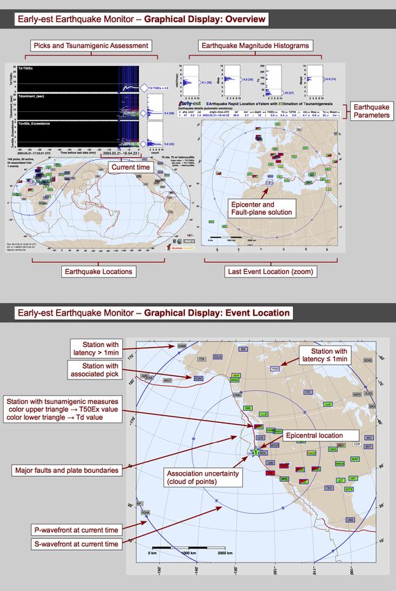
2020                                                                                       F. Bernardi: Early-est performance

ulation or securing critical facilities such as nuclear power      national seismic network and exchanges seismic data in real
plants. With advance evacuation plans and well-informed            time with a number of international seismic data providers.
communities, tsunami warnings could also be sent directly          The Istituto Superiore per la Protezione e Ricerca Ambi-
to the population.                                                 entale (ISPRA) maintains the national sea level network
   Reliable tsunami warnings should be disseminated as fast        and provides real-time data to the INGV monitoring room.
as possible in order to also be effective for the coastal areas    The implemented tsunami warning procedure uses the Early-
very close to the earthquake source, since a tsunami may ar-       est software developed by Lomax and Michelini (2009a, b,
rive at these areas within the first few minutes after the event   2011, 2012) to rapidly detect, locate, and determine the mag-
origin time. Populations exposed to tsunami hazards in the         nitude for large to great regional and teleseismic earthquakes.
field near to the source, however, should be aware that the           The purpose of this paper is to analyze the performance of
time between warning issuance and tsunami impact may be            Early-est regarding past events, in order to evaluate its reli-
too short to escape the tsunami; warning may arrive even           ability for the near-real-time tsunami warnings disseminated
after the tsunami, or the system may be subject to failure         by the INGV, and eventually tune the procedure as a whole.
for several reasons. Hence, the population should know how            INGV CTSP follows the ICG/NEAMTWS guidelines.
to self-evacuate relying on natural warnings when they are         ICG/NEAMTWS rules establish that a CTSP must dissem-
present, such as strong and/or unusually long shaking, ocean       inate a tsunami message, with warning levels that depend
withdrawal, an anomalously rising tide, roaring sounds from        on location, magnitude, and depth of the earthquake accord-
the ocean, etc.                                                    ing to a decision matrix, for all earthquakes with magnitudes
   To provide the earliest possible alerts, initial warnings       M ≥ 5.5 in their zone of competence. Messages are sent for
from regional tsunami warning systems are normally only            earthquakes that are large and shallow enough, and which
based on seismic information. Thus, fast, precise, and re-         occur in sea areas or inland but are sufficiently close to the
liable earthquake source parameters like epicenter coordi-         coast to possibly generate a tsunami. INGV is responsible for
nates, hypocenter depth, and magnitude are crucial for seis-       the earthquake and tsunami source zone extending from the
mologically based tsunami early warning procedures. This           Gibraltar Strait in the west, to Marmara and Levantine seas
is particularly important in the Mediterranean Sea, where          to the east.
the tsunami wave travel times between source regions and              The seismicity in the Mediterranean region is moderate to
coastlines are short and dedicated deep-sea instruments, such      high but also includes M = 8+ earthquakes that occurred in
as DART® buoys (http://nctr.pmel.noaa.gov/Dart/), to be in         the past and generated significant tsunamis (Maramai et al.,
place.                                                             2014; Lorito et al., 2015). It is difficult to assess if M = 9-
   The Istituto Nazionale di Geofisica e Vulcanologia              class earthquakes might occur, and these can not be ex-
(INGV) in Italy is a Candidate Tsunami Service Provider            cluded (Kagan and Jackson, 2013). Even if tsunamigenic
(CTSP) in the framework of ICG/NEAMTWS (NEAMTWS,                   earthquakes are likely to occur, their time recurrence inter-
2011), which is the tsunami early warning and mitigation           vals are however quite long (Koravos et al., 2003; Jenny et al.,
system established by IOC/UNESCO for the northeastern              2004; Bungum and Lindholm, 2007); moreover, the Mediter-
Atlantic, the Mediterranean and connected seas. For this rea-      ranean Sea is a relatively small area, and earthquakes with
son, the Centro Allerta Tsunami (CAT) (Italian for “tsunami        M ≥ 5.5 do not occur very frequently. The Global CMT cat-
alert center”), was established at the INGV headquarter in         alogs (Dziewonski et al., 1981; Ekström et al., 2012) include
Rome at the end of 2013. The CAT mission is to implement           about 125 earthquakes with Mw ≥ 5.5 within the Mediter-
and maintain a 24/7 service alongside the ordinary seismic         ranean region, which implies an occurrence rate of ≈ 30 ev-
surveillance of the national territory, and to work towards a      ery 10 years. Early-est has now been running for several
probabilistic seismic hazard assessment (PSHA) for the Ital-       years, but only since the beginning of March 2012 has its
ian coasts, that is a tsunami hazard map for seismically in-       current major version release been online and its solutions
duced tsunamis (Basili et al., 2013). CAT-INGV started op-         have been able to be systematically archived; thus we have
erations on a 24/7 basis as a CTSP in October 2014. Monthly        few events to analyze for tuning our tsunami alert procedure
communication tests are performed with national authorities,       (Table 1). For this reason, we perform our analysis using all
subscriber IOC member states, and other institutions, such as      earthquakes which have occurred worldwide and have been
the DG-ECHO Emergency Response Coordination Center in              located by Early-est since March 2012. To perform the analy-
Brussels. In the NEAM region there are three other CTSPs in        sis and tune our procedure, we proceed by comparing the epi-
operation: CENALT in France, NOA in Greece, and KOERI              centers, the hypocenter depths, and the estimation of magni-
in Turkey. IPMA, in Portugal, should begin operations soon.        tudes provided fully automatically by Early-est with the same
Each of these CTSPs has its specific competence source ar-         parameters provided by other agencies taken as a reference.
eas within the NEAM region.                                        Such agencies provide manually validated/revised locations
   At the national level, INGV is responsible for issuing mes-     and magnitude estimations for earthquakes on a global scale.
sages to the Civil Protection authority, which is presently re-       This paper is structured as follows: in the next section, we
sponsible for alert dissemination. INGV also maintains the         give a brief overview of the Early-est algorithm, in Sect. 3 we

Nat. Hazards Earth Syst. Sci., 15, 2019–2036, 2015                         www.nat-hazards-earth-syst-sci.net/15/2019/2015/
F. Bernardi: Early-est performance                                                                                                      2021

Table 1. List of earthquakes that occurred in the Mediterranean region located by Early-est with M ≥ 5.5 between March 2012 and December
2014. For each event we have listed the computed event origin time, epicenter coordinates, hypocenter depth, the maximum 68 % confidence
error in xyz space (in kilometers), the preferred magnitude (mb, Mwp or Mwpd ), and a reference magnitude, i.e., when the first Early-est
locations were available (in seconds) after the event origin time, and when the magnitudes stabilize (in minutes) after the first location was
available. A magnitude is stable when the difference to the final magnitude is ≤ ∓0.2.

       No.        Date         Time        Lat.    Long.     Depth      δ(xyz)   Magbest       Magref              First     First
                                                                                                                location   magnitude
         1     2012-06-10     12:44:15    36.36    28.93      19.7       4.3     Mwp = 6.1      CMT = 6.1
                                                                                               Mw                   167         10
         2     2012-09-12     03:27:43    34.77    24.08      10.0       5.1     mb = 5.7      mbNc = 5.4           201         7
         3     2013-01-08     14:16:09    39.62    25.49      10.1       4.2     Mwp = 5.7      CMT = 5.7
                                                                                               Mw                   174          3
         4     2013-06-15     16:11:02    34.51    24.99      15.4       5.4     Mwp = 6.4      CMT
                                                                                               Mw    = 6.3          181         2
         5     2013-06-16     21:39:07    34.51    25.00      18.6       4.8     Mwp = 6.1      CMT = 6.0
                                                                                               Mw                   117         3
         6     2013-10-12     13:11:51    35.52    23.30      11.5       5.2     Mwp = 6.6      CMT = 6.8
                                                                                               Mw                   194         2
         7     2013-12-28     15:21:06    36.04    31.30      56.8       8.5     Mwp = 6.0      CMT = 5.9
                                                                                               Mw                   358         5
         8     2014-01-26     18:45:10    38.29    20.38      19.8       2.5     mb = 5.2       Nc = 5.4
                                                                                               Mw                   115         3
         9     2014-02-03     03:08:46    38.25    20.40      10.1       2.3     Mwp = 6.1      CMT = 6.0
                                                                                               Mw                    77         7
        10     2014-04-04     20:08:07    37.26    23.71      115.9      2.2     mb = 5.5       CMT = 5.6
                                                                                               Mw                   119         6
        11     2014-05-24     09:25:03    40.23    25.34      10.1       4.8     Mwp = 6.6      CMT
                                                                                               Mw    = 6.9          124         7
        12     2014-08-29     03:45:06    36.75    23.67      81.2       2.7     Mwp = 5.8      CMT = 5.8
                                                                                               Mw                   119         4

Table 2. Global earthquake catalogs used for the analysis in this          phase association, event detection, hypocenter location, and
work. For each catalog we have indicated the begin and end time            event characterization. This characterization (Table A1) in-
of the time window of the data set included in this work. Catalog          cludes mb and Mwp magnitudes, the determination of ap-
abbreviations used in this paper are in brackets in the first column.      parent rupture duration, T0 , large earthquake magnitude,
                                                                           Mwpd , and the assessment of tsunamigenic potential us-
     Catalog                  Begin      End               Type            ing Td and T50 Ex, as described in Lomax and Michelini
     Early-est (EEc)          03-2012    12-2014     automatic             (2009a, b, 2011). The Early-est program reads Mini-SEED
     NEIC (Nc)                01-2004    12-2014       revised             data packets from a file or a SeedLink server (http://ds.iris.
     GFZ (Gc)                 06-2006    12-2014       revised             edu/ds/nodes/dmc/services/seedlink, http://www.seiscomp3.
     CSEM (Cc)                10-2004    12-2014       revised             org/wiki, doc/applications/seedlink), and passes each packet
     PTWC (Pc)                12-2013    06-2014       revised
     CMT-Harvard (CMT)        01-1976    10-2014       revised
                                                                           to a trace-processing module. The program also runs an
                                                                           associate/locate-reporting module at regular reporting inter-
                                                                           vals (e.g., after all data are read by Mini-SEED; every 1 min
                                                                           for SeedLink). The Early-est software maintains a persistent
describe the data set used in our analysis, and in the three sec-          pick list for the current reporting window (e.g., the last hour
tions following that, we then analyze and compare the earth-               before real time) and an event list for a specified archive in-
quake source parameters provided by Early-est with the ones                terval (e.g., the last 10 days). The pick list is updated con-
provided by the reference agencies; first the epicenter loca-              tinuously as picking and trace processing are applied to new
tion (Sect. 4), then the hypocenter depth (Sect. 5), and lastly            data packets. The event list is updated at each reporting inter-
the magnitude (Sect. 6). In Sect. 7 we will analyze the speed              val as new event locations are found or previous locations are
performances of Early-est with respect to the location and                 deleted. At each reporting interval, the associate/locate mod-
the magnitude parameters, in order to set the timeline of our              ule processes the current pick list from scratch, without mak-
automatic tsunami warning procedure. Lastly, we present the                ing use of previous associations or location information from
discussions and conclusions.                                               the event list; this memory-less procedure simplifies the as-
                                                                           sociate/locate module and makes it very robust with respect
                                                                           to changes in the pick list, but increases the computational
2   Early-est algorithm description                                        load. To reduce this load, the persistence of association and
                                                                           location information for well located events is currently be-
Early-est is a software package for rapid location and                     ing added to Early-est.
seismic/tsunamigenic characterization of earthquakes. The
Early-est software package operates using offline-event or
continuous-real-time seismic waveform data to perform trace
processing and picking, and, at a regular report interval,

www.nat-hazards-earth-syst-sci.net/15/2019/2015/                                  Nat. Hazards Earth Syst. Sci., 15, 2019–2036, 2015
2022 F. Bernardi: Early-est performance
2.1 Trace-processing module 3 Data set
The trace-processing module processes each new data packet The Early-est catalog (EEc in this paper) includes fully au-
passed by the Early-est program. This processing includes tomatic and unrevised location and magnitude estimations
channel identification, quality control, filtering for picking, for 5449 events from around the globe recorded at regional
picking, and further filtering and pre-processing as required and teleseismic distance with magnitude M&5.0. The cur-
for seismic and tsunamigenic event characterization (Ta- rent major version release of Early-est has been running since
ble A1). the beginning of March 2012. Our analysis will use locations
Picking in Early-est is performed by FilterPicker (Lomax and magnitudes for events which occurred between the be-
and Michelini, 2012; Vassallo et al., 2012), a general pur- ginning of March 2012 and the end of December 2014. At
pose, broadband, phase detector and picker which is appli- the beginning of March 2012, Early-est was using about 300
cable to real-time seismic monitoring and earthquake early seismic broadband stations. The number of stations has con-
warning. FilterPicker uses an efficient algorithm which op- tinuously been increasing, and at the end of September 2014
erates stably on continuous, real-time, broadband signals, the Early-est software was using a virtual station network of
avoids excessive picking during large events, and produces 494 stations (Fig. 1).
onset timing, realistic timing uncertainty, onset polarity, and We use the following as reference catalogs: (i) the
amplitude information. In practice, it operates on a prede- catalog provided by GEOFON project of the Deutches
fined number of frequency bands by generating a set of band- GeoForschungsZentrum (Gc in this paper, http://geofon.
passed time series with different center frequencies. Charac- gfz-potsdam.de/eqinfo/form.php); (ii) the catalog provided
teristic functions are determined for each frequency band and by the US National Earthquake Information Center (Nc in
a pick is declared if and when, within a window of predefined this paper); (iii) the catalog provided by the EMSC-CSEM
time width, the integral of the maximum of the characteristic (Cc in this paper) (http://www.emsc-csem.org/Earthquake),
functions exceeds a predefined threshold. (Godey et al., 2007); (iv) the catalog provided by the Global
After picking for each new data packet, for each pick in the CMT project (CMTc in this work) (Dziewonski et al., 1981;
pick list for the current packet channel, the trace-processing Ekström et al., 2012); (v) and the catalog provided by the Pa-
module applies various analyses on the channel data and up- cific Tsunami Warning Center (Pc in this paper) provided to
dates values needed for event characterization. Recursive, the authors of this paper courtesy of Barry Hirshorn of the
time-domain algorithms are used for all filtering and other Pacific Tsunami Warning Center (http://ptwc.weather.gov).
time-series processing. The CMTc and the Pc will be used specifically to compare
and assess the Mwp and Mwpd magnitudes.
2.2 Associate/locate-reporting module The above-mentioned observatories and centers provide
manually verified and/or revised earthquakes source param-
The Early-est associate/locate-reporting module runs an oc-
eters for different time periods. Table 2 summarizes the ab-
tree associate/locate module with the current pick list, and
breviations and time windows for each catalog used in this
then the reporting module which determines event character-
work. The ICG/NEAMTWS guidelines indicate that tsunami
ization results and generates graphical and alpha-numeric re-
warning must be disseminated for all events in the Mediter-
porting output. The octree associate/locate module efficiently
ranean and northeastern Atlantic regions with M ≥ 5.5. For
and robustly associates picks, and detects and locates seismic
this reason, although Early-est locates events with magnitude
events over the whole Earth from 0 to 700 km depth using
M&5.0, our analysis will focus only on worldwide earth-
the efficient, nonlinearized, probabilistic and global, octree
quakes with magnitude M ≥ 5.5.
importance-sampling search (Lomax et al., 2001, 2009). See
Appendix A for more details.
The Early-est reporting module processes the current pick
4 Epicenter location
list and event list to determine event characterization results
(Table A1) and generate graphical, alpha-numeric, XML,
In this section, we use the three reference catalogs Nc, Gc,
HTML, and other reporting output for events, picks, stations,
and Cc, and the Early-est catalog EEc.
etc. An e-mail or other alert message can be generated for
We first build three couples with the three reference cata-
each event with magnitudes or tsunamigenic potential that
logs (Gc–Cc, Cc–Nc and Gc–Nc) and we compute the dis-
exceed preset thresholds. Figure A1 shows the main graphi-
tance between the epicenter coordinates for each earthquake
cal display of Early-est, which summarizes the evolving trace
listed in both catalogs for each couple.
processing, associate/locate module and event characteriza-
The top panel in Fig. 2 shows the histograms represent-
tion results in real time.
ing the distributions of the location differences in each cou-
ple from the reference catalogs. The M ≥ 5.5 earthquakes
are generally located with mean distance differences smaller
than δ1ref .20 ∓ 25 km; almost 95 % of all earthquakes are
Nat. Hazards Earth Syst. Sci., 15, 2019–2036, 2015 www.nat-hazards-earth-syst-sci.net/15/2019/2015/F. Bernardi: Early-est performance 2023
−120˚ −80˚ −40˚ 0˚ 40˚ 80˚ 120˚ 160˚ −160˚
80˚ 80˚
60˚ 60˚
40˚ 40˚
20˚ 20˚
0˚ 0˚
−20˚ −20˚
−40˚ −40˚
−60˚ −60˚
−80˚ −80˚
−120˚ −80˚ −40˚ 0˚ 40˚ 80˚ 120˚ 160˚ −160˚
Figure 1. Global map with the 494 seismic broadband stations used by Early-est (the list is updated at the end of September 2014). The
stations belong to 45 different networks providing data in real time. When working in real time, latencies in the data stream and/or connection
problems may occur, reducing the number of waveform available for location and magnitude estimation.
located with distance differences of δ1ref .50 km. We did 5 Hypocenter depth
not find evidence for geographical and/or tectonic depen-
dence of this uncertainty. In this section we proceed as described in the section above:
We then compare the epicenter coordinates between the we use the three reference catalogs Nc, Gc, and Cc and the
earthquakes listed in the EEc and each of the three reference Early-est catalog EEc to build the catalog couples used in
catalogs (Fig. 2, bottom panels), i.e., we build the couples the previous section. We then compute the depth difference
EEc-Cc, EEc-Nc, and EEc-Gc. The histograms show that the between the hypocenters for each earthquake listed in both
epicenter location differences between the EEc and the ref- catalogs of each couple.
erence catalogs δ1EEc are similar to the differences plotted Figure 3 (top panels) shows histograms that represent the
on the top panels. The mean location difference between the distribution of the depth differences in each couple from
EEc and the reference catalogs is about δ1EEc .20 ∓ 20 km the reference catalogs. The hypocenter depth estimation for
and 95% of all events in the data set show differences earthquakes with magnitude M ≥ 5.5 listed in global cata-
δ1EEc .45 km. logs is generally well resolved: the mean and standard devia-
Generally our analysis showed that earthquakes with M ≥ tions difference are δZref ≈ 0∓25 km for all catalog couples.
5.5 can be located by using seismic data from global net- We did not find evidence for geographical and/or tectonic de-
works, with an empirical uncertainty, defined as the mean pendence of these differences.
location difference with respect to the reference catalogs, of We then compare the hypocenter depths between the EEc
about ν ≈ 20 ∓ 25 km. and each of the three reference catalogs (Fig. 3 bottom pan-
els; couples EEc-Cc, EEc-Nc, and EEc-Gc). The bottom
panels show that the hypocenter depth estimation between
the Early-est catalog and the reference catalogs do not dif-
fer significantly: the mean difference distributions are about
δZEEc ≈ 0 ∓ 30 km.
www.nat-hazards-earth-syst-sci.net/15/2019/2015/ Nat. Hazards Earth Syst. Sci., 15, 2019–2036, 20152024 F. Bernardi: Early-est performance
1200 1750 1200
Gc Nc Cc Nc Gc Cc
1000 µ = 17 ± 22 1500 µ = 16 ± 24 1000 µ = 15 ± 16
95th = 45 95th = 51 95th = 41
1250
800 800
No. RIff events
1000
600 600
750
400 400
500
200 200
250
0 0 0
0 20 40 60 80 100 0 20 40 60 80 100 0 20 40 60 80 100
∆o [km] ∆o [km] ∆o [km]
250 250 250
EEc Cc EEc Nc EEc Gc
µ = 18 ± 15 µ = 18 ± 17 µ = 18 ± 18
200 200 200
95th = 41 95th = 42 95th = 43
150 150 150
No. RIff events
100 100 100
50 50 50
0 0 0
0 25 50 75 100 0 25 50 75 100 0 25 50 75 100
∆o [km] ∆o [km] ∆o [km]
Figure 2. Epicenter location difference distributions for the events listed in the reference and in the Early-est catalogs. The epicenter location
difference is expressed in kilometers on the x axis. The y axis refers to the number of events for each bin; the bins are 5 km each. The top
panels show the location difference between the locations of the three reference catalogs: Nc, Gc, and Cc. The bottom panels show the location
difference between Early-est and the reference catalogs. The gray color scale indicates magnitude ranges as follows: dark gray 5.5 ≤ M < 6,
middle dark gray 6.0 ≤ M < 6.5, middle light gray 6.5 ≤ M < 7.0 and light gray M ≥ 7.0. The mean and the standard deviation and the
95 % percentiles for the entire dates (i.e., regardless of the magnitude) are indicated on the top right of each panel.
Generally, our analysis showed that hypocenter depth of Table 3. Early-est computes mb, Mwp , and Mwpd . This table sum-
earthquakes with M ≥ 5.5 can be precisely estimated when marize the rules used by Early-est to define the best magnitude
using seismic data from global networks, with an empirical (i.e., the most significative magnitude type) between mb, Mwp , and
uncertainty of about ν ≈ 00 ∓ 30 km. Mwpd . The magnitude mb is computed using the 30 s time window
or the apparent source duration To as a time window when To < 30 s
and using the IASPEI WWSSN-SP response for convolution. The
magnitude Mwp is scaled to the largest of the first two maxima on
6 Magnitude integrated displacement within the window from tP to tP + To time
or 120 s after tP , where tP is the P -arrival time – whichever window
Early-est provides three different types of magnitude: mb, is the shortest. The magnitude Mwpd (duration–amplitude), which
Mwp , and Mwpd (Lomax and Michelini, 2011) and then au- can be viewed as an extension of the Mwp moment-magnitude al-
tomatically decides each minute which magnitude type is the gorithm, is computed following the Mwp procedure and corrections
most significant, following the rules in Table 3. The criteria described in Lomax and Michelini (2012).
to assign the best magnitude listed in Table 3 follow two sim-
ple principles: (i) a minimum number of observations is re- Best magnitude #1 Magnitude range2
quired to obtain reliable magnitude estimations, and (ii) mag- Mwpd ≥6 Mwp ≥ 7.2
nitude types are reliable within magnitude ranges. Follow- Mwp ≥6 5.8 ≤ Mwp < 7.2
ing Lomax and Michelini (2009a, b, 2011) we set the va- mb ≥6 Mwp < 5.8
lidity range 5.8 ≤ Mwp < 7.2 for the best magnitude; mb is 1 : number of recording stations with good signal-to-noise
assigned to best magnitude when Mwp < 5.8 and Mwpd is ratio and reliable amplitude reading. 2 : magnitude range
assigned to best magnitude when Mwp > 7.2 In this work validity
we compare the Early-est magnitude types Mwp and Mwpd
with the reference magnitude types Mwp , and Mw . Since the
Nat. Hazards Earth Syst. Sci., 15, 2019–2036, 2015 www.nat-hazards-earth-syst-sci.net/15/2019/2015/F. Bernardi: Early-est performance 2025
1500 1500
Gc Nc Cc Nc Gc Cc
1250 µ = -4 ± 22 1250 µ = 3 ± 16 1250 µ = -2 ± 21
5th = -38 5th = -21 5th = -34
NRRIoo events
1000 95th = 25 1000 95th = 30 1000 95th = 30
750 750 750
500 500 500
250 250 250
0 0 0
−100−75 −50 −25 0 25 50 75 100 −100−75 −50 −25 0 25 50 75 100 −100−75 −50 −25 0 25 50 75 100
∆Z [km] ∆Z [km] ∆Z [km]
400 400 400
EEc Cc EEc Nc EEc Gc
µ = 0 ± 26 µ = 1 ± 24 µ = 0 ± 27
300 5th = -36 300 5th = -29 300 5th = -35
95th = 31 95th = 35 95th = 34
NRRIoo events
200 200 200
100 100 100
0 0 0
−100−75 −50 −25 0 25 50 75 100 −100−75 −50 −25 0 25 50 75 100 −100−75 −50 −25 0 25 50 75 100
∆Z [km] ∆Z [km] ∆Z [km]
Figure 3. Hypocenter depth difference distributions for the events listed in the reference and in the Early-est catalogs. The hypocenter depth
difference is expressed in kilometers on the x axis. The y axis refers to the number of events for each bin; the bins are 5 km each. The top
panels show the hypocenter depth difference distribution between the locations of the three reference catalogs Nc, Gc, and Cc. The bottom
panels show the hypocenter depth difference between Early-est and the reference catalogs. The gray color scale indicates magnitude ranges
as follows: dark gray 5.5 ≤ M < 6, middle dark gray 6.0 ≤ M < 6.5, middle light gray 6.5 ≤ M < 7.0, and light gray M ≥ 7.0. The mean
and the standard deviation and the 95% percentiles for the entire dates (i.e., regardless of the magnitude) are indicated on the top right of
each panel.
ICG/NEAMTWS guidelines prescribe that for earthquakes magnitudes provided by Early-est differ significantly from
with depth Z ≤ 100 km, a standard general warning should the magnitudes provided by the reference catalogs. The over-
only be delivered for events with M ≥ 5.5, and no action estimation and the wider distribution appear to be homoge-
should be taken for smaller magnitudes, we only analyze the neously distributed among all magnitude ranges.
magnitude comparisons for events with Z ≤ 100 km in this In the next subsections, we will analyze the magnitude val-
section. ues for each single magnitude type mb and Mwp separately
As in Sects. 4 and 5 we first compare the magnitudes pro- in more detail.
vided by the reference catalogs. Then, we compare the mag-
nitudes provided by Early-est with the magnitudes listed in 6.1 mb
the reference catalogs. First we will compare all best mag-
nitude (i.e., mb or Mwp ) results, only considering couples In this subsection we compare the mbEE magnitudes pro-
between catalogs where the magnitude types are identical vided by Early-est to the mb magnitudes provided by NEIC
(Fig. 4). This comparison will provide a general overview on (mbNc ) and EMSC (mbCc ). We use the mbEEc only when
how the best magnitudes of Early-est match with the magni- Early-Est assigns the best magnitude to mb, following the
tudes from the reference catalogs. rules of Table 3.
Figure 4 shows the distribution of the magnitude differ- Figure 5 shows the mbEEc with respect to the mbNc (top
ences δM EEc = M EEc − M ref between the values of the EEc left panel) and with respect to the mbCc (top right panel).
and the ones from the reference catalogs. These two plots show scattered and sparse distributed val-
When comparing the Early-est magnitudes with the mag- ues, which are coherent with the magnitude differences of the
nitudes from the two reference catalogs (Fig. 4), Early-est histograms in Fig. 4c and d. The mean δmb indicates that the
seems to overestimate the magnitudes by about δM EEc ≈ catalogs are coherent, but the standard deviation and the per-
0.1 ∓ 0.2. The percentiles show that more than 10 % of the centiles point out that the mbEEc can be significantly under-
estimated or overestimated with respect to mbNc and mbCc .
www.nat-hazards-earth-syst-sci.net/15/2019/2015/ Nat. Hazards Earth Syst. Sci., 15, 2019–2036, 20152026 F. Bernardi: Early-est performance
200 200
EEc Cc EEc Nc
µ = 0.08 ± 0.22 µ = 0.10 ± 0.23
150 150
5th = -0.25 5th = -0.24
95th = 0.44 95th = 0.44
No. RIff events
100 100
50 50
0 0
−0.6 −0.4 −0.2 0.0 0.2 0.4 0.6 −0.6 −0.4 −0.2 0.0 0.2 0.4 0.6
�M �M
Figure 4. Magnitude difference distributions for the events listed in the EEc catalog compared to the two Nc and Cc reference catalogs.
Differences are computed only when the same magnitude type is provided for the same event in the two compared catalogs. The magnitude
difference is on the x axis. The y axis refers to the number of events for each bin; the bins are 0.1 magnitude each. The color scale refers to
the same magnitude ranges as in Figs. 3 and 2, and not to the magnitude type. The gray color scale indicate magnitude ranges as follows: dark
gray 5.5 ≤ M < 6, middle dark gray 6.0 ≤ M < 6.5, middle light gray 6.5 ≤ M < 7.0, and light gray M ≥ 7.0. The mean and the standard
deviation and the 95 % percentiles for the entire dates (i.e., regardless of the magnitude) are indicated on the top left of each panel.
In order to correct such scattered and sparse distribution, uncertainty between the two reference catalogs (Fig. 4, left
we computed a linear regression function for each panel panel).
(thick dashed lines on the top panels). These functions are
computed for f1 = mbEEc → mbNc and for f2 = mbEEc → 6.2 Mwp
mbCc . The constant a and b of the linear function are shown
in the upper left corners of Fig. 4a and b. We then applied the As a reference, we first compare the magnitudes Mwp Pc values
regression functions f1 and f2 to the mbEEc values and we re- provided by the Pacific Tsunami Warning Center (PTWC)
compute the differences (third row of the histograms). Both using the correction of Whitmore et al. (2002) with the
new distributions have mean values close to 0 and smaller MwCMTc of the CMT-Harvard catalog (Fig. 6). The magni-
standard deviation and percentiles compared to the original tudes compare well with a mean difference µ = 0.04 ∓ 0.19
ones. for events with magnitude about Mwp .7.0–7.5. For larger
The two functions appear similar but show different a events, the magnitudes Mwp Pc begin to overestimate with re-
and b constants. In order to test if such differences are
spect to the MwCMTc .
significant, first we applied the function f1 , derived for EEc with the M CMTc
We now compare the magnitudes Mwp
mbEEc → mbNc , and we computed the differences with re- EEc
w
spect to the mbCc values. Secondly, we applied the func- (Fig. 7). The Mwp magnitudes appear to be significantly
tion f2 , derived for mbEE → mbCc , and we computed the overestimated (> 0.2 magnitude unit) for earthquakes with
residuals with respect to the mbNc values. Applying these MwCMT ≤ 6.5.
corrections, we obtain two new difference distributions: Mwp is based on the far-field approximation to the
δmbEEc→Nc and δmbEE→Cc (bottom left and right pan- P wave displacement due to a double-couple point source
Cc Nc
EE→Nc (Tsuboi et al., 1995), thus we should consider that the re-
els). The δmb and δmbEEc→Nc
Cc distributions, and
EE→Cc sult of Mwp computed in the field near to the source may be
the δmb and the δmbEE→Cc
Nc distributions appear to biased. In fact Hirshorn et al. (2012) showed that single sta-
be significantly different. We performed a t test between tion Mwp values measured at stations at epicentral distances
δmbEE→Nc and the δmbEEc→Nc Cc distribution and between 1 ≤ 15◦ have positive residuals with respect to the Harvard
δmbEEc→Nc
Cc and δmb EEc→Cc
Nc . The null hypothesis Ho is re- centroid moment tensor Mw . Nevertheless, our procedure is
jected at more than 95 %. built to obtain reliable Mwp estimates as fast as possible, thus
From the percentiles of the corrected distributions, partic- we aim to also use Mwp measured from stations close to the
ularly on the left side, we observe that when applied, the re- epicenter.
gression function f1 produces a narrower magnitude differ- EEc values may be dependent as a function
To test if our Mwp
ence distribution with respect to the function f2 . of the distance between station and epicenter, we plotted the
Generally, after applying the linear corrections, the result- station residuals at each station for each event with respect to
ing mbEE uncertainty (ν ≈ 0.00 ∓ 0.14), with respect to the the epicenter distance (Fig. 8). Station residuals are defined
reference catalogs, is coherent with the overall magnitude as δMwpi = M EEc,i − M CMTc , where i indicates the M
wp w wp val-
ues measured at each station.
Nat. Hazards Earth Syst. Sci., 15, 2019–2036, 2015 www.nat-hazards-earth-syst-sci.net/15/2019/2015/F. Bernardi: Early-est performance 2027
(a) (b)
(c) (d)
(e) (f)
(g) (h)
Figure 5. Magnitude mb differences between the Early-est catalog and the reference catalogs (Nc on the left and Cc on the right). Top row
panels (a) and (b) depict mb magnitude comparison between the Early-est values (x axis) and the reference catalog values (y axis). The
dashed lines refer to the linear regression functions, the a and b constant are indicated on the upper left corner, and the thin black line refers
to the 1 : 1 proportion. Second row panels (c) and (d) depict mb magnitude difference distribution; each bin is 0.05 R magnitude units wide.
The black line refers to the theoretical distribution derived from measured mean µ and standard deviation σ with = 1. Third row panels
(e) and (f) are as in the second row panels, but after applying the correction function, shown in the top panels, to the Early-est mb. Fourth
row panels (g) and (h) are as in the third row panels, but on the left panel, the EEc-Cc derived correction is applied and on the right panel,
the EEc-Nc derived correction is applied.
www.nat-hazards-earth-syst-sci.net/15/2019/2015/ Nat. Hazards Earth Syst. Sci., 15, 2019–2036, 20152028 F. Bernardi: Early-est performance
Figure 6. Comparison between the Mwp magnitudes computed by the Pacific Tsunami Warning Center (PTWC) and the Mw magnitudes
from the CMT-Harvard catalog. Plot on the left side: the dots denote magnitude values, the continuous line denotes the 1 : 1 ratio, and dashed
lines denote ∓0.2 uncertainty. The histogram on the right side shows the δMwp − Mw distribution. Mean, standard deviation, and percentiles
are indicated on the top right of the right panel. Each bin is 0.05 magnitude wide.
tomatic magnitude estimations within a few minutes after the
event origin time in order to disseminate early tsunami warn-
ings. Thus the closer stations are relevant and must be used.
For this reason we apply Eq. (1) to remove the distance
EEc,i
dependency of the measured Mwp and we then recompute
EEc
the magnitude events Mwp, corr . To recompute the Mwp, EEc
corr
we follow the Early-est procedure as follows: we cut off sta-
EEc,i EEc,i
tions with Mwp < 10th percentile and with Mwp > 10th
percentile. The event magnitude is Mwp = 50th percentile of
the remaining values. The bottom right histogram of Fig. 8
shows the corrected magnitude differences δMwp, EEc
corr . The
right shift of the original magnitude differences distribution
(Fig. 8, bottom left) is corrected. The resulting magnitude
MwpEEc uncertainty with respect to the M CMTc is δM
Figure 7. Early-est magnitudes Mwp compared with the CMT- w wp =
Harvard Mw from the CMT-Harvard catalog. The continuous line 0.0 ∓ 0.2, which is consistent with the uncertainty of the
indicates the 1 : 1 ratio and dashed lines indicate ∓0.2 uncertainty. Mwp provided by the PTWC with respect to the global CMT-
Harvard catalog.
The top left of Figure 8 shows the residuals δMwp i (gray
dots) for all events with hypocenter depth ≤ 100 km plotted 7 Speed performance and tsunami warning alert
with respect to the epicentral distance in degrees. From these timeline
residuals we compute the regression function (dashed line in
Fig. 8): In the previous section, we analyzed the final epicenter lo-
cation, hypocenter depth, and magnitude values provided by
f (1) = − 1.32e−6 · 13 + 2.40e−4 · 12
Early-est, i.e., the values obtained about 20 min to 1 h after
− 0.0146 · 1 + 0.314. (1) the event origin time. A tsunami alert however, is meaning-
ful when delivered within a short time after the event origin
i are overestimated
Figure 8 and Eq. (1) show that the δMwp time and with reliable earthquake source parameters. In order
for distances 1.30◦ and slightly underestimated for dis- to plan the timeline procedure at the CAT-INGV, we want to
tances 1&90◦ . After applying the regression function f (1) know how fast the earthquake source parameters computed
to the station values, the distance dependency of Mwp i is re-
by Early-est converge toward a stable value.
moved (Fig. 8 top right panel). We thus first analyze how fast Early-est provides a first
EEc,i
The distance dependency of the measured Mwp at each automatic location, and second, how fast the epicenter coor-
EEc with
station results in a general overestimation of the Mwp dinates and the magnitudes stabilize.
respect to the MwCMTc (Fig. 7 bottom left). The overesti- The histogram in Fig. 9 shows the delay time after the
mation of Mwp EEc could of course be removed using only event origin time when a first automatic location of Early-est
Mwp , measured at stations with epicentral distance 30◦ ≤ becomes available. We generally have to wait at least 2 min in
1 ≤ 90◦ . Nevertheless, Early-est is designed to provide au- order to have a first automatic solution; within 7 and 10 min
Nat. Hazards Earth Syst. Sci., 15, 2019–2036, 2015 www.nat-hazards-earth-syst-sci.net/15/2019/2015/F. Bernardi: Early-est performance 2029
Figure 8. Epicentral distance dependence of the Mwp for events with hypocentral depth ≤ 100 km. The top left panel shows station residuals
i = M EE,i − M CMT (gray dots), plotted with respect to the epicentral distance in degree, and the dashed line, which represents a third
δMwp wp w
degree polynomial regression function (Eq. 1) which best fits the data. The top right panel indicates station residuals δMwp i = M EEcorr,i −
wp
Mw CMT (gray dots), after applying the regression function (Eq. 1), plotted with respect to the epicentral distance in degree, and the dashed
line, which is a third degree polynomial regression function, which best fits the corrected residuals with respect to the distance. Bottom
left panel: event magnitude difference 1Mwp distribution before the distance correction. These distribution are similar to Fig. 7 as follows:
mean, standard deviation, and percentiles
R are indicated on the left of the histogram, bins are 0.5 magnitude wide each, and the black solid line
refers to theoretical distribution with = 1. The bottom right panel shows event magnitude difference 1Mwp corr distribution after the distance
correction using Eq. (1).
after the event origin time, about 95 and 100 % of all earth-
quakes are located, respectively. On a global scale, a large
number of earthquakes are located along the oceanic ridges
and trenches, which are far away from most of the seismic
stations. In the Mediterranean region, the distances between
earthquake sources and seismic stations are generally shorter
than on a global scale. Table 1 lists the 12 events with magni-
tude M ≥ 5.5 that occurred in the Mediterranean region be-
tween March 2012 and the end of December 2014. These
12 events do not form a reliable statistic, but from Table 1
we may reasonably expect to locate an event in the Mediter-
ranean region with magnitude M ≥ 5.5 within 2–3 min after
the event origin time.
Figure 9. Early-est first location performance. This figure shows
how fast a first location for global events is available through Early- Figure 10 shows how fast a first location (top panel) and
est. The bins (25 s wide) on the x axis refer to the seconds after magnitude (bottom panel) stabilizes towards the final and sta-
the event origin time (OT) when a first location is available. On the ble values.
top right, the mean, the standard deviation, and four representative Both panels indicate that for most of the events, the epicen-
percentiles are indicated. ter coordinates and magnitudes within the first 8–10 min after
the first available location may be considered stable and sig-
nificantly close to the final values, since the magnitudes are
www.nat-hazards-earth-syst-sci.net/15/2019/2015/ Nat. Hazards Earth Syst. Sci., 15, 2019–2036, 20152030 F. Bernardi: Early-est performance
40
mean + SD
mean
30
km 20
10
0
0 5 10 15 20 25 30 35 40 45 50 55 60
0.5
mean + SD
mean
0.4
Magnitude Unit
0.3
0.2
0.1
0.0
0 5 10 15 20 25 30 35 40 45 50 55 60
Figure 10. Early-est location and magnitude estimation stability performances. This figure shows how fast a first location estimation (top
panel) and magnitude (bottom panel) estimations evolve towards stable values. Top panel: for each run, we computed the distance in kilo-
meters between the current epicenter and the epicenter of the last location. Bottom panel: for each run we computed the absolute magnitude
difference between the current magnitude and the final magnitude. In this panel, most of the magnitudes are available 2 min after the event
origin time, since often the first automatic location may not provide a magnitude value. The magnitude refers to the “best” magnitude decided
by Early-est (Table 3) at each run. In both panels difference values (depicted by black crosses) are plotted on the y axis with respect to the
minutes after the first location is established (0 value at the x axis). The black line depicts the mean value computed for each minute and the
dashed line shows the mean plus the standard deviation.
µ + σ ≤ 0.2 and the epicenter locations are µ + σ ≤ 10 km, fifth and the eighth locations available after the first loca-
respectively. tion is established. Considering that the first location in the
The CAT-INGV uses the earthquake source parameters Mediterranean region may be available within 2–3 min af-
provided by Early-est to compile the tsunami warning mes- ter the event origin time, the second, the fifth and the eighth
sages to be disseminated to the civil authorities. The mission locations may be available by about 5, 8, and 11 min after
of the CAT is to provide tsunami warnings for earthquakes the event origin time. Therefore, in the case of an earthquake
with M ≥ 5.5 which occur in the Mediterranean region ac- in the Mediterranean region, the continuous monitoring of
cording to the ICG/NEAMTWS guidelines. Early-est provides information to the seismologists for issu-
Based on the speed performances of Early-Est on comput- ing tsunami warnings. Based on Fig. 10 and Table 1, such a
ing reliable earthquake source parameters (Fig. 10) and on procedure may be executed within about ≈ 15 min after the
the minimum delay time after the event origin time to lo- event origin time. The messages are delivered via several me-
calize an event in the Mediterranean (Table 1), we set the dia such as mail, fax, GTS (https://www.wmo.int/pages/prog/
timeline described below to allow fast enough production of www/TEM/GTS), and SMS. This ensures that messages are
warning messages based on robust seismic estimates. typically delivered to authorities within seconds.
Based on Fig. 10 we decided to automatically compile a
tsunami warning alert message always for the second, the
Nat. Hazards Earth Syst. Sci., 15, 2019–2036, 2015 www.nat-hazards-earth-syst-sci.net/15/2019/2015/F. Bernardi: Early-est performance 2031
8 Discussions and final remarks computed mb values produces indeed a reduction of the
standard deviation to about ∓0.15 units of magnitude. Both
Early-est is able to provide a first location within about f1 and f2 corrections help the avoidance of large magni-
7 min from the origin time for almost 95 % of all worldwide tude over- and underestimations. The f1 correction function
earthquakes. In the Mediterranean region, where the epicen- shows slightly more narrow distribution than the f2 correc-
tral distance between the earthquake and the seismic station tion function.
is smaller, we may expect a first automatic location result Nevertheless, the mb magnitude starts to saturate from a
within 2–3 min after the event origin time. Generally within magnitude of mb &6.0, and for this reason Early-est does not
less than 10 min after the first location is established, the es- use mb when Mwp ≥ 5.8. Thus, mb values apply to earth-
timations converge to stable values. quakes which are not generally expected to be tsunamigenic.
In our analysis, the automatic locations and source depth The Early-est magnitude Mwp values are reliable
estimates provided by Early-est for global M ≥ 5.5 earth- when computed using only stations with epicentral dis-
quakes are robust and reliable; in fact the epicenter source tance 30◦ ≤ 1 ≤ 90◦ . As expected (Tsuboi et al., 1995;
parameters estimates by Early-est are coherent with the Hirshorn et al., 2012), single station Mwpi measurements at
◦
epicenter source parameters provided after manual revi- distance 1 ≤ 30 are significantly overestimated (Fig. 8).
sion/validation by other agencies (NEIC, GFZ, and CSEM- The observed distance-dependent bias at each station results
EMSC) that locate earthquakes on a global scale. in a general overestimation of the final Mwp (Fig. 7). Early-
Generally our analysis showed that earthquakes with M ≥ est is designed to provide automatic magnitude estimation
5.5 can be located by using seismic data from global net- within a few minutes after the event origin time in order to
works, with an empirical uncertainty, defined as the mean disseminate early tsunami warnings, thus the closer stations
location difference with respect to the reference catalogs, of are relevant and must be used. For this reason we prefer to
about ν ≈ 20 ∓ 25 km. The locations provided by Early-est correct the station Mwp values to remove the overestimation
show differences to the locations from the reference catalogs, of the single station Mwp values at distance 1 ≤ 30◦ , instead
that are comparable to the location differences among the ref- of introducing a minimum distance cut off.
erence catalogs. Since the assignment rules for the best magnitude depend
A similar conclusion is valid for the mean Early-est focal on the number of stations measuring reliable mb, Mwp , and
depth difference for global M ≥ 5.5 earthquakes, which is Mwpd and the magnitude value for each one (Table 3), the
about ν ≈ 0 ∓ 25 km, which is also coherent with the focal assigned best magnitude may vary between mb, Mwp , and
depth differences between the reference catalogs. Mwpd at each run. This is particularly true within the first
Early-est uses only a subset of all worldwide, public, real- few minutes after the event origin time, when the number of
time stations, and the fact that the available number of sta- available waveforms may still be small, and the magnitude
tions sometimes may be reduced because of latencies does values may not be stable yet (Fig. 10). The linear correction
not seem to affect the quality of the estimated epicenter co- for mb and the distance-dependent correction for Mwp will
ordinates and hypocenter depth. thus produce a stable and reliable best magnitude useful for
The magnitude is a key earthquake parameter to determine seismologically based tsunami early warning procedures.
the tsunami alert level (see Sect. 1). The decision matrix de- The CAT-INGV provides seismologically based tsunami
fined by the NEAMTWS (2011) sets the tsunami warning early warnings when earthquakes with magnitude M ≥ 5.5
level on the basis of the magnitude, hypocenter depth, and occur in the Mediterranean region. Such tsunami warning
the distance between the epicenter and the coastal forecast messages are based on the fully automatically location and
points. The automatic mb and Mwp magnitudes provided by magnitude estimations provided by the Early-est software.
Early-est show differences to the reference values used, that The analysis of a data set of 3 years of worldwide earth-
in some cases may be significant in the context of a tsunami quakes showed that Early-est is a robust, reliable, and effi-
warning. cient piece of software for automatic real-time earthquake
The mb magnitudes provided by Early-est compare well source parameter estimation, which provides reliable and ro-
with the mb values provided by reference catalogs from the bust location parameters and magnitude estimations within a
point of view of the mean differences, but show sparse and few minutes after the event origin time.
scattered distributions that can be larger than ∓0.3 units of
magnitude. Such sparse distribution can be corrected by in-
creasing the signal-to-noise ratio threshold for the mb sta-
tion values. On the other hand, a higher signal-to-noise ra-
tio threshold may reduce the number of station readings, and
would require more stations to obtain a reliable mb value.
This would result in a slower magnitude estimation, which
may affect the efficiency and the speed required for the dis-
semination of tsunami warnings. A linear correction of the
www.nat-hazards-earth-syst-sci.net/15/2019/2015/ Nat. Hazards Earth Syst. Sci., 15, 2019–2036, 20152032 F. Bernardi: Early-est performance
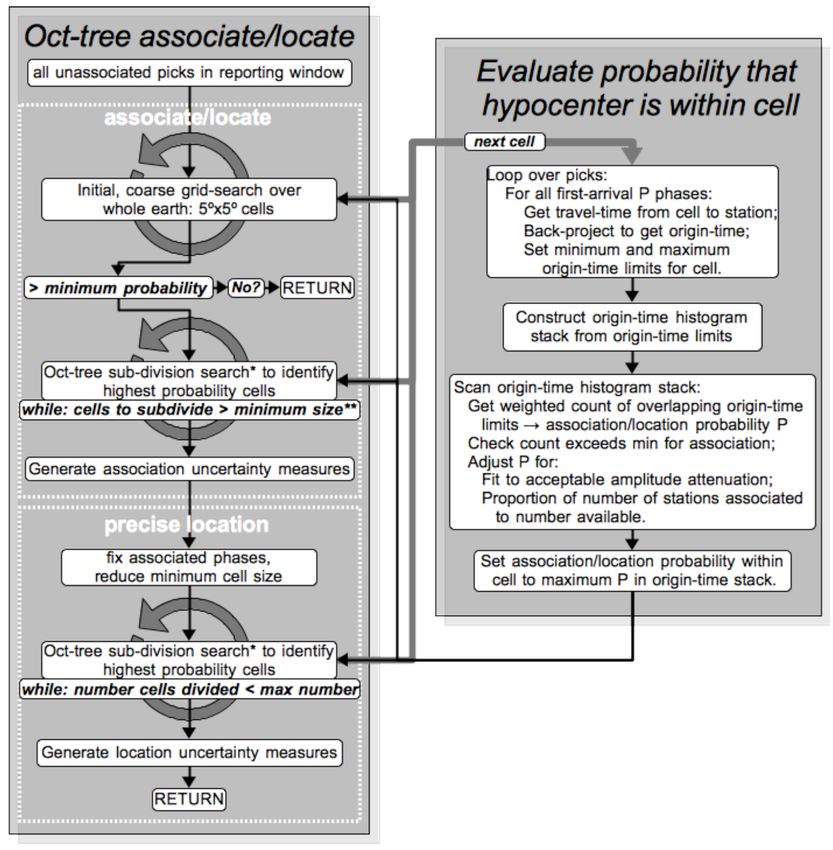
Appendix A: Octree associate/locate module tance, and azimuth distributions, then P (x, v) is stored for
use in the progression of the octree search. If any of these
The octree associate/locate module (Fig. A2) efficiently and conditions are not met, then the octree associate/locate mod-
robustly associates picks, and detects and locates seismic ule returns with a flag that no event has been associated.
events over the whole Earth from 0 to 700 km depth using P (x, v) represents the relative probability that an event is lo-
the efficient, nonlinearized, probabilistic, and global octree cated within a cell of volume v at position x.
importance-sampling search (Lomax et al., 2001, 2009). The The octree search to associate/locate is paused when the
objective function for the octree search is a probability func- subdivided cells reach an adaptively determined, minimum
tion, P (x), based on the stacking of implicit origin times size (e.g., ≤ 5 km for a location constrained by regional
for each pick for each potential source x test . Given a seismic to globally distributed stations, ≤ 1 km for a location con-
wave velocity model (currently ak135 Kennett et al., 1995), strained by locally distributed stations); in this pause, uncer-
a pick time tp at a seismic station, and assuming a seismic tainty measures (e.g., PDF scatter samples) are generated in
phase type that may have produced the pick, the phase travel- the association stage. The octree search and cell subdivision
time from the source x test to the station Tx can be calculated is then continued for a fixed number of samples (currently
and thus the implicit origin time T0 for the source and phase about 4600) to obtain a refined, precise location by fixing the
can be determined by back projection (e.g., T0 = Tp − Tx ). associated phases to those corresponding to the maximum of
The set of stacks of T0 for all picks forms a histogram over the P (x, v) found in the association stage. The fixing of the
potential origin times for a source at x test . If the maximum associated phases is necessary for small cell sizes since a de-
histogram value exceeds a specified threshold, and if the as- creasing cell volume combined with the step-function limits
sociated picks for the maximum pass tests on amplitudes and on origin time leads to a continuous reduction in P (x, v) val-
station distributions, then P (x test ) is retained to drive the oc- ues and eventual instability and nonconvergence of the octree
tree search further to find a maximum x max = max[P (x)] search near and at the optimal source location. The precise
and define a seismic event at x max and associated picks. octree results provide uncertainty measures (e.g., PDF scat-
The octree search is direct and nonlinearized – it does ter samples, uncertainty ellipsoid) for the location.
not involve linearization of the equations relating the pick When the octree associate/locate module returns an event,
times to the source location, and is global and probabilistic; the associated picks for this event are masked in the pick list
it samples throughout the prior probability density function and the octree associate/locate module is run again using the
(PDF) for the seismic location problem. The search uses an remaining, non-associated picks, until no further events are
initial, coarse, regular grid-search followed by recursive, oc- returned. Thus multiple events can be associated and located
tal sub-division, and sampling of cells in three-dimensional, within a report interval, and, in general, the events are iden-
latitude/longitude/depth space to generate a cascaded, octree tified in order of the number of associated picks and better
structure of sampled cells. The octree search produces ap- location constraint.
proximate importance-sampling – the spatial density of sam- Early-est runs the octree associate/locate module every
pled cells follows the objective function P . 1 min using all picks from the past hour, without knowl-
For each latitude/longitude/depth cell of volume v scanned edge of or preserving information from previously associ-
by the octree search, a histogram-like stack over implicit ori- ations and event locations. This procedure makes Early-est
gin times for first-arrival, P phases (currently Pg, P , Pdiff, relatively simple algorithmically, and robust with regards to
PKPdf), is constructed for all picks in the pick list. Each changes in the set of available picks and the number of as-
origin-time value T0 is assigned a distance and pick-quality- sociated picks defining locations. In particular, this proce-
weighted amplitude A between 0 and 1.0, and an uncertainty dure allows early stage locations with few associated picks
σ determined by the sum of half the maximum travel-time to easily move in space or origin time, or to split in multiple
range across the cell volume with the travel-time and pick events, or to be absorbed in other events, or to disappear as
uncertainties. Each implicit origin time is included in the more pick data become available. However, this procedure is
origin-time stack with amplitude A using two step-function inefficient for later stage event locations which are defined
time limits at T0 ∓ σ inserted in time order. After all picks by a larger number of associated picks, e.g., more than 10–
have been processed, the maximum of the origin-time stack 20 picks, since such locations are very unlikely to change;
is found by a systematic scan over the available time limits; much processing effort is repeated each minute to reobtain
the use of step-function time limits and time ordering makes a previous result. This inefficiency can be problematic after
this scan very fast. All picks whose origin time limits over- large earthquakes, when the repeated re-processing of hun-
lap the stack maximum time are flagged as associated. The dreds of picks from a mainshock and large aftershock can
stack value, combined with the variance of the implicit ori- cause Early-est to fall behind real time.
gin times from all associate picks, is converted to a probabil-
ity, P (x, v). If the maximum stack value exceeds a specified
threshold (currently 4.5), and if the associated picks for the
maximum pass tests on amplitude attenuation, station dis-
Nat. Hazards Earth Syst. Sci., 15, 2019–2036, 2015 www.nat-hazards-earth-syst-sci.net/15/2019/2015/You can also read