Visualizing Functional Data With an Application to eBay's Online Auctions
←
→
Page content transcription
If your browser does not render page correctly, please read the page content below
Visualizing Functional Data With an
Application to eBay’s Online Auctions

Wolfgang Jank1 , Galit Shmueli1 , Catherine Plaisant2 , and Ben
Shneiderman2
1
    Department of Decision and Information Technologies
    Robert H. Smith School of Business
    University of Maryland
    College Park, MD 20742 USA
    {wjank,gshmueli}@rhsmith.umd.edu
2
    Human-Computer Interaction Laboratory
    Department of Computer Science
    University of Maryland
    College Park, MD 20742 USA
    {plaisant, ben}@cs.umd.edu

1 Introduction

The technological advancements in measurement, collection, and storage of
data have led to more and more complex data-structures. Examples include
measurements of individuals’ behavior over time, digitized 2- or 3-dimensional
images of the brain, and recordings of 3- or even 4-dimensional movements of
objects travelling through space and time. Such data, although recorded in
a discrete fashion, are usually thought of as continuous objects represented
by functional relationships. This gives rise to functional data analysis (FDA),
made popular by the monographs of Ramsay and Silverman (1997, 2002),
where the center of interest is a set of curves, shapes, objects, or, more gener-
ally, a set of functional observations. This is in contrast to classical statistics
where the interest centers around a set of data vectors. In that sense, func-
tional data is not only different from the data-structure studied in classical
statistics, but it actually generalizes it. Many of these new data-structures
call for new statistical methods in order to unveil the information that they
carry.
    There are many examples of functional data. The year-round tempera-
ture at a weather station can be thought of as a continuous curve, starting
in January and ending in December, where the amplitude of the curve sig-
nifies the temperature-level at each day or at each hour. Then, a collection
of temperature-curves from different weather stations is a set of functional
data. Similarly, the price during an online auction for a certain product can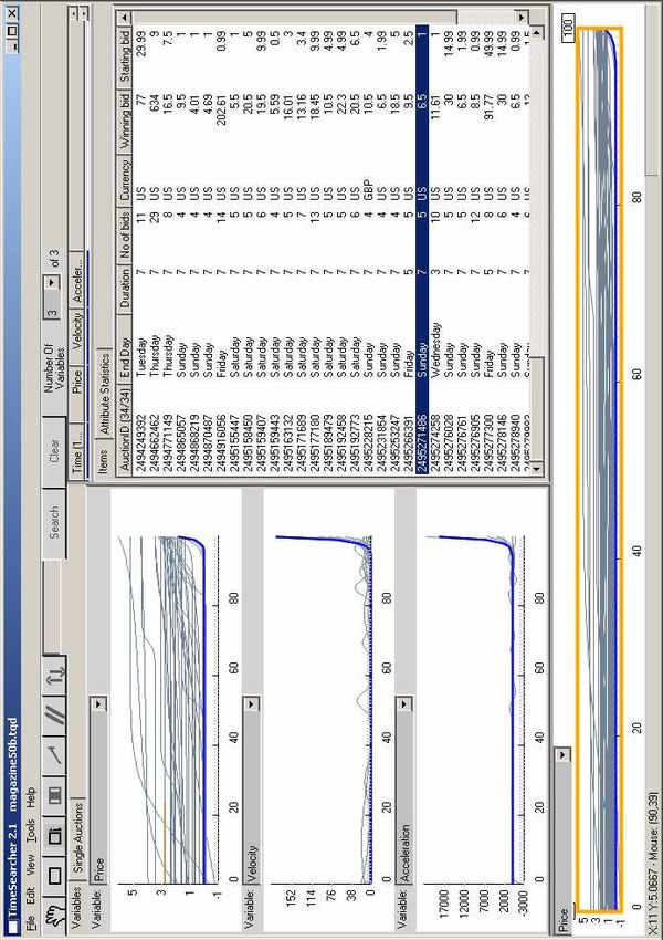
2      Jank, Shmueli, Plaisant, and Shneiderman

be represented by a curve, and a sample of multiple auction price curves for
the same product is then a set of functional objects. Alternatively, the digi-
tized image of a car passing through a highway toll-booth can be described by
a 2-dimensional curve measuring the pixel-color or -intensity of that image.
The collection of image-curves from all cars passing the toll-booth during a
single day could then again be considered as a set of functional data. Lastly,
the movement of a person through time and space can be described by a 4-
(or even higher) dimensional hyperplane in x-, y-, z- and time-coordinates.
The collection of all such hyperplanes from people passing through the same
space is again a set of functional data.
    Data-visualization is an important part of any statistical analysis and it
serves many different objectives. Visualization is useful for understanding the
general structure and nature of the data such as the types of variables con-
tained in the data (categorical, numerical, text, etc.), their value ranges, and
the balance between them. Visualization is useful for detecting missing data
and it can also aide in pinpointing extreme observations and outliers. More-
over, unknown trends and patterns in the data are often uncovered with the
help of visualization. After identifying such patterns, they can then be in-
vestigated more formally using statistical models. The exact nature of these
models (e.g. linear vs. log-linear) is again often based on insight learned from
visualization. And finally, model assumptions are typically verified through
visualization of residuals and other model-related variables.
    While visualization is an important step in understanding any data, dif-
ferent types of data require different types of visualizations. Take for instance
the example of cross-sectional data vs. time-series data. While the informa-
tion in cross-sectional data can often be displayed satisfactorily with the help
of standard bar charts, boxplots, histograms or scatter-plots, time-series data
require special graphs that can also capture the temporal information. The
methods used to display time-series data range from rather simple time-series
plots, to streaming video clips for discrete time-series [Mills et al., 2005], to
cluster- and calendar-based visualization for more complex representations
[van Wijk and van Selow, 1999].
    Functional data are different from ordinary data in both structure and
concept and thus require special visualization methods. While the objectives
in visualizing functional data are similar to those of ordinary data, functional
data arrive with additional challenges that require extra attention. One such
challenge is with respect to the creation of functional observations. Functional
data are typically obtained by recovering the continuous functional object
from the discrete observed data via data-smoothing. The implication of this
is that there are two levels to the study of functional data. The first level
uses the discrete observed data to recover the continuous functional object.
Visualizing data at this level is important for detecting anomalies that are
related to the data generation process, such as data collection and data entry,
as well as for assessing the fit of the smoothed curves to the discrete observed
data. This is illustrated and discussed further in Section 3. The second and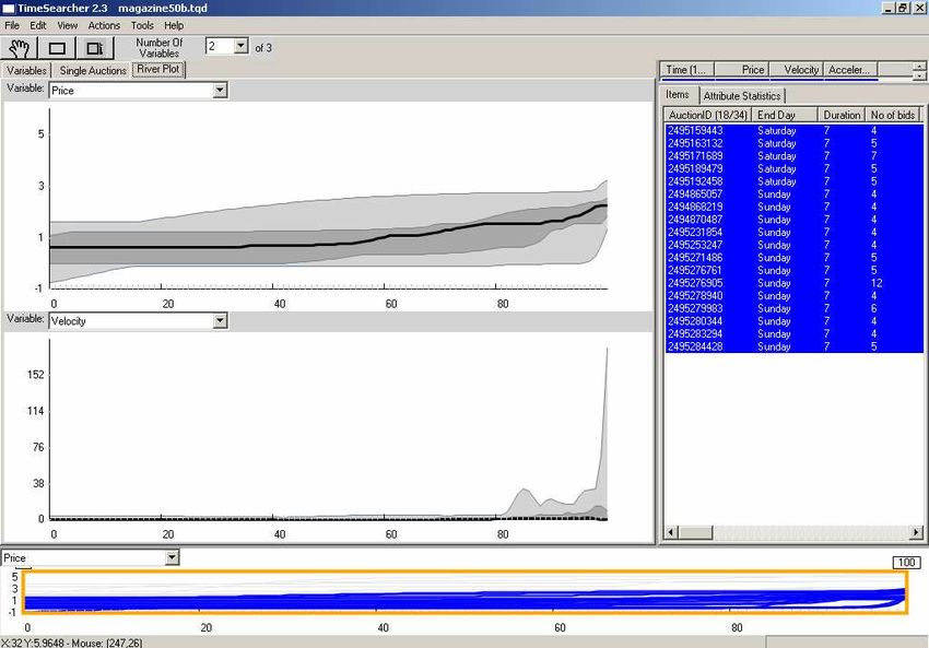
Functional Visualization      3

higher level of study operates on the functional objects themselves. Since on
this level the functional objects are the observations of interest, visualization
is now used for the same purposes described earlier for ordinary data: for
detecting patterns and trends, possible relationships, and also for detecting
anomalies. In Section 4 we describe different visualizations that enhance the
understanding of the data and that support more formal analyses.
    Visualizing functional data has not received much attention in the lit-
erature to date. Most of the literature focuses on the derivation of mathe-
matical models for functional data, with visualization playing a minor role
and typically appearing only as a side product of the analysis. Some note-
worthy exceptions include the display of summary statistics such as the
mean and the variability of a set of functional objects, the use of phase-
plane plots to understand the interplay of dynamics, and the graphing of
functional principal components to study sources of variability within func-
tional data [Ramsay and Silverman, 2002]. Another exception is the work of
[Shmueli and Jank, 2005] and [Hyde et al., 2005] which is focused directly on
the visualization of functional data, and which suggests a few novel ideas for
the display functional data such as calendar plots and rug plots.
    Most of the existing visualizations for functional data are static in na-
ture. By static we mean that once a graph is generated it can no longer be
modified by the user without re-running a piece of software code. A static
approach is useful for differentiating subsets of curves by attributes (e.g., by
using color), or for spotting outliers. A static approach however does not al-
low for an interactive exploration of the data. By interactive we mean that
the user can perform operations such as zooming in and out, filtering the
data and obtaining details for the filtered data, and do all of this from within
the graphical interface. Interactive visualizations for the special structure of
functional data are not straightforward, and solutions have been considered
only recently [Aris et al., 2005, Shmueli et al., 2005]. In Section 5 we describe
an interactive visualization tool designed for the display and exploration of
functional data. We illustrate its features and benefits using the example of
price curves capturing the price evolution in online auctions.
    The insightful display of functional data arrives with many, many different
challenges, and we are only scraping the tip of the iceberg in this essay. Func-
tional data is challenging with respect to high object dimensionality, complex
functional relationships and concurrency among the functional objects. We
discuss some of these extra challenges in Section 6.

2 Online Auction Data from eBay
eBay (www.eBay.com) is one of the major online marketplaces and currently
the biggest consumer-to-consumer online auction site. eBay offers a vast
amount of rich bidding data. Besides the time and amount of each bid placed,
eBay also records plenty of information about the bidders, the seller, and
4 Jank, Shmueli, Plaisant, and Shneiderman
the product being auctioned. On any given day, several million auctions take
place on eBay and all closed auctions from the last 15 days are made publicly
available on eBay’s Web site. This huge amount of information can be quite
overwhelming and confusing to the user (i.e. either the seller, the potential
buyer, or the auction house) who wants to incorporate this information into
his/her decision-making process. Data visualization can help alleviate this
confusion.
Online auctions lend themselves naturally to the use of functional data
for a variety of reasons. Online auctions can be conceptualized as a series
of bids placed over time. The finite time horizon of the auction allows the
study of the price evolution between the start and the end of the auction. By
price evolution we mean the progress of price due to a new bid as the auction
approaches its end. Conceptualizing the price evolution as a continuous price
curve allows the researcher to investigate price dynamics via the price curve’s
first and second derivatives.
It is noteworthy that empirical research of online auctions has been, for the
most part, ignoring the temporal dimension of the bidding data, and instead
has been looking only at a condensed snapshot of the auction. That is, most
research has considered only the auction end by, for example, concentrating
only on the final price rather than on the entire price curve, or by looking only
at the total number of bidders rather than the function describing the bidder
arrival process. Looking only at the auction end leads to information loss since
such an approach entirely ignores the way in which that end was reached.
Functional data analysis is a natural solution to avoid this information loss.
In a recent series of papers the first two authors have taken a functional
approach and shown that the price evolution paired with its dynamics leads to
a better understanding of different auction profiles [Jank and Shmueli, 2005]
or to more accurate forecasts of the final auction price [Wang et al., 2005].
3 Visualization at the Object Recovery Stage
Any functional data set consists of a collection of continuous functional objects
such as a set of continuous curves describing the temperature changes over
the course of a year, or the price increases in an online auction. Despite their
continuous nature, limitations in human perception and measurement capa-
bilities allow us to observe these curves only at discrete time points. Moreover,
the presence of human and measurement error results in discrete observations
that are noisy realizations of the underlying continuous curve. Thus, the first
step in every functional data analysis is to recover, from the observed data,
the underlying continuous functional object. This is typically done with the
help of smoothing techniques.
A variety of different smoothers exist. One very flexible and computation-
ally efficient choice is the penalized smoothing spline [Ruppert et al., 2003].
Let τ1 , . . . , τL be a set of knots. Then, a polynomial spline of order p is givenFunctional Visualization 5
by
X
L
f (t) = β0 + β1 t + β2 t2 + . . . + βp tp + βpl (t − τl )p+ , (1)
l=1
where u+ = uI[u≥0] denotes the positive part of the function u. Define the
roughness penalty Z
PENm (t) = {Dm f (t)}2 dt, (2)
where Dm f , m = 1, 2, 3, . . ., denotes the mth derivative of the function f . The
penalized smoothing spline f minimizes the penalized squared error
Z
PENSSλ,m = {y(t) − f (t)}2 dt + λ PENm (t), (3)
where y(t) denotes the observed data at time t and the smoothing parameter
λ controls the trade-off between data-fit and smoothness of the function f .
Using m = 2 in (3) leads to the commonly encountered cubic smoothing
spline. Other possible smoothers include the use of B-splines or radial basis
functions [Ruppert et al., 2003].
The process of going from observed data to functional data is now as
follows. For a set of n functional objects, let tij denote the time of the
jth observation (1 ≤ j ≤ ni ) on the ith object (1 ≤ i ≤ n), and let
yij = y(tij ) denote the corresponding measurements. Let fi (t) denote the pe-
nalized smoothing spline fitted to yi1 , . . . , yini . Then, functional data analysis
is performed on the continuous curves fi (t) rather than on the noisy obser-
vations yi1 , . . . , yini . That is, after creating the functional objects fi (t), the
observed data yi1 , . . . , yini are discarded and subsequent modeling, estimation
and inference are based on the fi (t)’s only.
One important implication of this practice is that any error or inaccuracy
in the smoothing step will propagate into inference and conclusions based
on the functional model. What makes matters worse is a) that the observed
data are discarded after the functional data are created and thus often hard
to retrieve, and b) that any violation of the functional model is confounded
with the error at the smoothing step. That is, it is hard to know whether a
model violation is due to model mis-specification or, rather, due to anomalies
at the smoothing step. For that reason, it is important to carefully monitor
the functional object recovery process and to detect inaccuracies early in the
process using appropriate tools. Although there exist measures for evaluat-
ing the goodness of fit of the functional object to the observed data (such as
those based on residual sums of squares, or criteria that include the rough-
ness penalty), it is unwise to rely on these measures alone, and visualization
becomes an indispensable tool in the process.
Consider Figures 1-3 for illustration. The Figures compare recovered func-
tional objects under three different smoothing scenarios. Specifically, for bid-
ding data from 16 different eBay online auctions, Figure 1 shows the resulting6 Jank, Shmueli, Plaisant, and Shneiderman
Functional Object 1 Functional Object 5 Functional Object 9 Functional Object 13
6
6
6
6
5
5
5
5
4
4
4
4
3
3
3
3
2
2
2
2
0 1 2 3 4 5 6 7 0 1 2 3 4 5 6 7 0 1 2 3 4 5 6 7 0 1 2 3 4 5 6 7
Functional Object 2 Functional Object 6 Functional Object 10 Functional Object 14
6
6
6
6
5
5
5
5
4
4
4
4
3
3
3
3
2
2
2
2
0 1 2 3 4 5 6 7 0 1 2 3 4 5 6 7 0 1 2 3 4 5 6 7 0 1 2 3 4 5 6 7
Functional Object 3 Functional Object 7 Functional Object 11 Functional Object 15
6
6
6
6
5
5
5
5
4
4
4
4
3
3
3
3
2
2
2
2
0 1 2 3 4 5 6 7 0 1 2 3 4 5 6 7 0 1 2 3 4 5 6 7 0 1 2 3 4 5 6 7
Functional Object 4 Functional Object 8 Functional Object 12 Functional Object 16
6
6
6
6
5
5
5
5
4
4
4
4
3
3
3
3
2
2
2
2
0 1 2 3 4 5 6 7 0 1 2 3 4 5 6 7 0 1 2 3 4 5 6 7 0 1 2 3 4 5 6 7
Fig. 1. Creating functional objects: price curves using penalized smoothing splines
with p = 2 and λ = 0.001.
functional objects via penalized smoothing splines using spline-order p = 2
and a small smoothing parameter λ = 0.001. Figure 2 on the other hand
corresponds to the same spline-order (p = 2) but a larger smoothing param-
eter (λ = 1). In Figure 3 we use spline-order p = 4, smoothing parameter
λ = 10 and a data pre-processing step via interpolation. The exact details of
the smoothing are not the center of interest here and can be found elsewhere
[Jank and Shmueli, 2005]. What is of interest here though is the fact Figures
1-3 correspond to three different approaches of recovering functional objects
from the same data. The researcher could have taken either one of these three
approaches and used the resulting functional objects for subsequent analy-
sis. However, as we will explain next, two of the three approaches lead to
very unrepresentative functional objects and thus, very likely, to erroneous
conclusions.
Statistical conclusions typically make sense only in the context of their
application and ignorance thereof will lead to wrong conclusions. This is no
different for visualizations. As mentioned earlier, Figures 1-3 show bidding
data from 16 eBay auctions. All auctions lasted 7 days. The circles correspond
to the observed bids (i.e. their timing and magnitude) while the solid lines
correspond to the resulting functional objects via penalized smoothing splines.
The objective in this stage is to recover, from the observed bidding data, the
underlying price curve. The price curve describes the price evolution duringFunctional Visualization 7
Functional Object 1 Functional Object 5 Functional Object 9 Functional Object 13
6
6
6
6
5
5
5
5
4
4
4
4
3
3
3
3
2
2
2
2
0 1 2 3 4 5 6 7 0 1 2 3 4 5 6 7 0 1 2 3 4 5 6 7 0 1 2 3 4 5 6 7
Functional Object 2 Functional Object 6 Functional Object 10 Functional Object 14
6
6
6
6
5
5
5
5
4
4
4
4
3
3
3
3
2
2
2
2
0 1 2 3 4 5 6 7 0 1 2 3 4 5 6 7 0 1 2 3 4 5 6 7 0 1 2 3 4 5 6 7
Functional Object 3 Functional Object 7 Functional Object 11 Functional Object 15
6
6
6
6
5
5
5
5
4
4
4
4
3
3
3
3
2
2
2
2
0 1 2 3 4 5 6 7 0 1 2 3 4 5 6 7 0 1 2 3 4 5 6 7 0 1 2 3 4 5 6 7
Functional Object 4 Functional Object 8 Functional Object 12 Functional Object 16
6
6
6
6
5
5
5
5
4
4
4
4
3
3
3
3
2
2
2
2
0 1 2 3 4 5 6 7 0 1 2 3 4 5 6 7 0 1 2 3 4 5 6 7 0 1 2 3 4 5 6 7
Fig. 2. Creating functional objects: price curves using penalized smoothing splines
with p = 2 and λ = 1.
an auction, and its derivatives measure the price dynamics. In that sense, the
objective is to create a functional object that is representative of the evolution
of price between the start and end of the 7-day auction. The process of bidding
on eBay follows an ascending format and the price curve should naturally
reflect that. This goal is somewhat complicated by the fact that observed
bids are not monotonically increasing due to eBay’s proxy bidding system
[Jank and Shmueli, 2005]. Thus, creating representative functional objects is
not a straightforward task.
Consider Figure 1. We can see that the functional objects are very “wiggly”
and certainly do not do a good job of representing the monotone price increase
in the auction. Moreover, we also notice that some of the objects (e.g. #2 and
#10) only partially cover the 7-day period and thus do not represent the price
evolution over the entire auction. The reason is in this case software-specific:
the penalized spline module pspline in R, by default, returns a function that
is defined only on the range of the input data. Hence, since for #2 and #10
the bids cover only a small part of the auction duration, so does the resulting
functional object. And lastly, we notice that there exist no functional objects
for #7 and #9. The reason for this is that the pspline module requires at
least 2p + 1 data points for estimation of a smoothing spline of order p. This
means that for an order-two smoothing spline we need at least (2)(2) + 1 = 5
points. However, both #7 and #9 only have 3 bids and thus no functional8 Jank, Shmueli, Plaisant, and Shneiderman
Functional Object 1 Functional Object 5 Functional Object 9 Functional Object 13
6
6
6
6
5
5
5
5
4
4
4
4
3
3
3
3
2
2
2
2
0 1 2 3 4 5 6 7 0 1 2 3 4 5 6 7 0 1 2 3 4 5 6 7 0 1 2 3 4 5 6 7
Functional Object 2 Functional Object 6 Functional Object 10 Functional Object 14
6
6
6
6
5
5
5
5
4
4
4
4
3
3
3
3
2
2
2
2
0 1 2 3 4 5 6 7 0 1 2 3 4 5 6 7 0 1 2 3 4 5 6 7 0 1 2 3 4 5 6 7
Functional Object 3 Functional Object 7 Functional Object 11 Functional Object 15
6
6
6
6
5
5
5
5
4
4
4
4
3
3
3
3
2
2
2
2
0 1 2 3 4 5 6 7 0 1 2 3 4 5 6 7 0 1 2 3 4 5 6 7 0 1 2 3 4 5 6 7
Functional Object 4 Functional Object 8 Functional Object 12 Functional Object 16
6
6
6
6
5
5
5
5
4
4
4
4
3
3
3
3
2
2
2
2
0 1 2 3 4 5 6 7 0 1 2 3 4 5 6 7 0 1 2 3 4 5 6 7 0 1 2 3 4 5 6 7
Fig. 3. Creating functional objects: price curves using data pre-processing via in-
terpolation of the bids and penalized smoothing splines with p = 4 and λ = 10.
object is created. This loss of information is quite disturbing from a conceptual
point of view since data for these two auctions is in fact available and the
missing (functional) data are a consequence of the functional object generation
process. In summary, if the researcher were to use the smoothing approach
from Figure 1 “blindly” (i.e. without careful checking of the results), then she
would obtain very unrepresentative functional objects and, in addition, loose
valuable information.
One reason for the poor representativeness of the objects in Figure 1 is
the low value of the smoothing parameter. Increasing λ to 1 (Figure 2) results
in much smoother (i.e. less wiggly) price curves. However, there still exist
partial functional objects (#2, #10) and missing functional objects (#7, #9).
Moreover, while the higher value of λ results in much less wiggly curves, some
of the functional objects now appear too inflexible (e.g. #15 may be considered
too close to a straight line).
We can achieve a better fit (i.e. more flexibility, yet little extra wiggli-
ness) by increasing the order of the spline together with the magnitude of
the smoothing parameter. We can also solve the problem of partial and miss-
ing functional objects by using a pre-processing step via interpolation. That
is, we interpolate the observed bidding data and fit the smoothing spline to
a discretized grid of the interpolating function [Jank and Shmueli, 2005]. In
that way, we can assure that we estimate the smoothing spline based on aFunctional Visualization 9
sufficient number of points that cover the entire range of the 7-day auction.
The result can be seen in Figure 3. Now, the functional objects appear to be
very representative of the price evolution, much better than in the previous
two approaches. Equally important, there are no more missing or partial func-
tional objects. Inference based on the objects in Figure 3 is likely to yield the
most reliable insight about the price evolution in online auctions.
The previous examples illustrate the importance of visualization at the
object recovery stage. Although the causes that lead to problems at this stage
may often be quite trivial (e.g. unfortunate software default settings or poor
parameter choices), they are typically hard to diagnose without the use of
proper visualizations.
4 Visualizing Functional Observations
4.1 Visualizing Individual Objects and their Dynamics
Mean Price and Confidence Bounds Mean Velocity and Confidence Bounds Mean Acceleration and Confidence Bounds
5.5
1.5
1.0
5.0
1.0
0.5
4.5
4.0
0.5
0.0
3.5
3.0
−0.5
0.0
2.5
−0.5
−1.0
2.0
0 1 2 3 4 5 6 7 0 1 2 3 4 5 6 7 0 1 2 3 4 5 6 7
Day of the Auction Day of the Auction Day of the Auction
Fig. 4. Summaries for functional objects: pointwise mean and 95% confidence
bounds for the price evolution, price velocity and price acceleration of the 16 eBay
online auctions.
Statistical analysis typically starts by scrutinizing data summaries and
graphs. Data summaries include measures of central tendency, variability,
skewness, etc. Traditionally, summary statistics are presented in numerical
form. However, in the functional setting each summary statistics is actually a10 Jank, Shmueli, Plaisant, and Shneiderman
functional object, such as the mean function or the standard deviation func-
tion. Since there usually exists no analytical, closed-form representation of
these functions, one resorts to graphical representation of the summary mea-
sures. The left panel in Figure 4 shows the (pointwise) mean price curve (solid
thick line) together with 95% upper and lower confidence curves (broken thick
lines) for the 16 auctions from Section 3. Since we only consider 16 auctions
in this example, one can easily identify the minimum and maximum prices
of all curves. In larger data sets, one may also want to add a curve for the
(pointwise) minimum and maximum, respectively.
One of the main advantages of functional data analysis is that it allows
for an estimation of derivatives. The nonparametric approach to the recov-
ery of the functional object guarantees that local changes in the data are
well-reflected, yet the object’s smoothness properties also allow for a reliable
estimation of partial derivatives. For instance, setting m = 4 in the penalty
term in (2) guarantees smooth first and second derivatives. Knowledge of the
derivatives can result in an important advantage, especially for applications
that experience change. Take the online auction setting as an example. While
the price curve f (t) describes the exact position of the price at any time point
t, it does not reveal how fast the price is moving. Attributes that we typically
associate with a moving object are its velocity (or its speed) and its accel-
eration. Velocity and acceleration can be computed via the first and second
derivatives of f (t), respectively. Knowledge of the dynamics can be impor-
tant for pinpointing the periods during which the auction price experiences
only little change which in turn is important for forecasting the final price
[Wang et al., 2005]. The middle and right panel of Figure 4 show velocity and
acceleration for the 16 eBay auctions together with the pointwise mean and
confidence bounds.
Another way of investigating the interplay of dynamics is with the help
of so-called phase plane plots. Phase plane plots graph dynamics against one
another. For instance, Figure 5 shows a graph of mean velocity versus mean
acceleration. The numbers on the curve indicate the day of the auction. We can
see that at the start (Day 0) high velocity is accompanied by low, negative
acceleration (=deceleration). Acceleration precedes velocity, so deceleration
now results in lower velocity tomorrow and consequently velocity decreases
to below 0.5 on day 1. This trend continues until acceleration turns positive
(between day 4 and day 5) causing velocity to pick up towards the auction end.
Phase plane plots are useful for diagnosing whether the interplay of dynamics
suggests a system that could be modelled by a suitable differential equation.
Another part of data exploration is investigating the distribution of indi-
vidual variables. Since most parametric models require the response to follow
a certain distribution (typically the normal distribution), this step is impor-
tant for selecting the right model and for assuring the appropriateness of
the selected model. One standard tool for investigating the distribution of a
numerical variable is the histogram. However, generalizing the idea of a his-
togram to the functional context is challenging since the input variable is aFunctional Visualization 11
Phase Plane Plot
0.15
7
0.10
6
0.05
5
Acceleration
0.00
−0.05
4
−0.10
3
2 1
−0.15
0
0.2 0.3 0.4 0.5 0.6
Velocity
Fig. 5. Phase plane plot of the mean velocity vs. the mean acceleration. The number
on the curve indicate the day of the auction.
Day 1 Day 4 Day 7
4
0.7
0.30
0.6
0.25
3
0.5
0.20
0.4
2
0.15
0.3
0.10
0.2
1
0.05
0.1
0.00
0.0
0
0 1 2 3 4 5 6 3.0 3.5 4.0 4.5 5.0 5.5 6.0 5.0 5.2 5.4 5.6 5.8 6.0
Fig. 6. Distribution of functional objects: histograms at day 1, 4 and 7 of a sample
of eBay online auctions. The grey line corresponds to a density estimate.
continuous function. One solution is to graph the distribution of the functional
object only at a few select snapshots in time. This can be done by discretizing
the object and graphing pointwise histograms (or similar plots such as prob-12 Jank, Shmueli, Plaisant, and Shneiderman
ability plots) at each time point. Figure 6 shows snapshots of the distribution
of a sample of eBay price curves at days 1, 4 and 7. These snapshots allow
conclusions about the distribution of the entire functional object.
4.2 Visualizing Relationships among Functional Data
Day 1 Day 4 Day 7
5.5
5
4
5.4
2
5.3
4
Log−Price
Log−Price
Log−Price
5.2
0
3
5.1
−2
5.0
2
4.9
−4
−4 −2 0 2 4 −4 −2 0 2 4 −4 −2 0 2 4
Log−Opening Price Log−Opening Price Log−Opening Price
Fig. 7. Relationship among functional objects: scatterplots of (log) price vs. (log)
opening bid at day 1, 4 and 7 of a sample of eBay online auctions. The solid grey
line corresponds to a scatterplot smoother with 3 degrees of freedom.
After examining each variable individually, the next typical step in ex-
ploratory data analysis is to investigate relationships across several variables.
For two numerical variables this is often accomplished with the help of scat-
terplots. One way of generalizing the traditional scatterplot to the functional
setting is, again, to graph a sequence of pointwise scatterplots. Figure 7 shows
scatterplots at days 1, 4 and 7 for the auction price versus the opening bid
(in log scale). We can see that the relationship between the two variables
changes over the course of time. While there exists a strong positive effect
at the beginning of the auction (left panel), the magnitude of the effect de-
creases at day 4 (middle panel), and there is barely any effect at all, possibly
even a slight negative effect, at the auction end (right panel). This suggests
that the relationship between the opening bid and the auction price may be
modelled well using a time-varying coefficient model. Of course, one aspect
that remains undiscovered in this pointwise approach is a possible 3-way in-
teraction between opening bid, price and time. Such an interaction could beFunctional Visualization 13
detected using a 3-dimensional scatterplot. However, as Figure 8 illustrates,
3-dimensional graphs have the disadvantage that they are not easy to read.
300
250
200
Day
7
Price
150
6
5
100
4
3
50
2
0
1
0 50 100 150 200 250
Opening Bid
Fig. 8. Relationship among functional objects: 3-d scatterplot of opening bid, price
and day of the auction.
4.3 Visualizing Functional and Cross-Sectional Information
As illustrated above, visualizing functional data is more challenging than vi-
sualization of classical data. The visualization process is often complicated
further by a coupling of functional observations with cross-sectional attribute
data. For example, online auction data include not only the bid history (i.e.
the timing and magnitude of bids), but also auction-specific attributes cor-
responding to auction design (e.g. length of the auction, magnitude of the
opening bid, use of a secret reserve price, use of the “Buy-It-Now” option,
etc.), bidder characteristics (e.g. bidder ID’s and ratings), seller character-
istics (e.g. seller ID and rating, seller location, whether or not a seller is a
“Powerseller,” etc.), and product characteristics (e.g. product category, prod-
uct quality and quantity, product description, etc). All of these characteristics
correspond to cross-sectional information in that they do not change during
the auction. The coupling of time-series with cross-sectional information is
important because the relationship between the two could be the main focus
or at least a partial focus of the analysis. Standard visualization tools are
geared either towards the display of time-series data alone or cross-sectional
data alone, but almost always not both.14 Jank, Shmueli, Plaisant, and Shneiderman
The combination of time-series and cross-sectional data into one display is
rare and requires careful, application-specific modifications of standard meth-
ods. Shmueli & Jank (2005) propose profile plots for displaying the temporal
sequence of bids together with additional auction attributes (such as a bidder’s
rating) in the same graph. This is illustrated in Figure 9, which describes the
sequence of bids in a 5-day eBay auction. The circle size is proportional to the
bidder’s eBay rating. However, profile plots are more suitable for visualizing
single auctions, and do not scale well.
250
200
150
Price ($)
100
50
0
0 1 2 3 4 5
Day of Auction
Fig. 9. Profile Plot of a single 5-day auction. The circles represent bids, with circle
size proportional to the bidder’s eBay rating.
Another type of plot that is suitable for visualizing functional data is the
rug plot [Hyde et al., 2005]. A rug plot displays curves (i.e. functional objects)
over calendar time in order to explore the effects of concurrency of events.
Figure 10 shows a rug plot displaying the price curves of 217 eBay auctions
for a Palm M515 PDA that took place over a 3-month period. The black
line represents the average daily closing price. We can see that daily prices
vary quite significantly and so does the daily price-variation (grey bands).
What’s more, we can see that there are time periods with many similar, almost
parallel price curves for same auction durations (e.g. 7-day auctions - green
curves - around 4/3 and also around 4/23). Moreover, the closing prices after
4/3 appear relatively low and so does the associated price-variability. Most
auctions closing at that time are 7-day auctions with similar shape. It would
be interesting to see if one could establish a more formal relationship between
similar price patterns (i.e. parallel price curves) and their effect on the price
and its uncertainty.
The rug plot in this example combines functional data with attribute data
via the time axis (calendar time on the x-axis takes into account the start and
end of the curve) and via color (different colors for different auction durations).
Notice that the plot scales well for a large number of auctions, but it is limited
in the number of attributes that can be coupled within the visualization.Functional Visualization 15
Price Evolution Curves Vs. Calendar Time
300
250
200
Price
150
100
50
0
3/14 3/24 4/3 4/13 4/23
Calendar Time
Fig. 10. Rug Plot displaying the price evolution (y-axis) of 217 online auctions over
calendar time (x-axis) during a 3-month period. The colored lines show the price
path of each auction with color indicating auction length (yellow = 3-day; blue=5-
day; green = 7-day; red = 10-day). The dot at the end of each line indicates the
final price of the auction. The black line represents the average of the daily closing
price , and the gray band is the inter-quartile range.
Finally, Trellis Displays [Cleveland et al., 1996] are another method that
supports visualizing relationships between functional and an attribute of inter-
est. This is done by displaying a series of panels where the functional objects
are displayed at different levels (or categories) of the attribute of interest (see,
for instance [Shmueli and Jank, 2005]). In general, while static graphs can
capture some of the relationships between time-series and cross-section infor-
mation, they become less and less insightful with increasing data dimension
and complexity. One of the reasons is that they have to accomplish mean-
ingful visualizations at several data-levels: relationships within cross-sectional
data (e.g. find relationships between the opening bid and a seller’s rating),
and within time-series data (e.g. find an association between the bid magni-
tudes, which is a sequence over time, and the number of bids, yet another
sequence over time). What complicates matters is that these graphs also have
to portray relationships across the different data types, for example, between
the opening bid and the bid magnitudes. In short, suitable graphs have to16 Jank, Shmueli, Plaisant, and Shneiderman
be very flexible to accommodate all the different data challenges. Ideally, one
would want to literally “dive” into the data and explore it interactively. By
interactive we mean that the user can perform operations such as zooming in
and out, filtering and obtaining details for the filtered data, and do all of this
from within the graphical interface.
Information visualization tools apply several common strategies to en-
able user control over data displays (see [Shneiderman and Plaisant, 2004],
[Card et al., 1999] or [Plaisant, 2005]). A primary strategy is by manipulat-
ing a set of widgets, such as dynamic query sliders that allow users to select
ranges of desired variables, often called conditioning. The power of interac-
tion is that users can rapidly (100msec) and incrementally change the ranges
to explore the effect on the display. For example, users can move a slider to
gradually eliminate auctions with low starting prices and see if that removes
time series plots that end with low, middle, or high closing prices. A second
strategy is to have multiple views of the data, e.g. scattergram, histograms
tabular, or parallel coordinate views. Then users can select a single or mul-
tiple items in one view and see the results in another view (“brushing”). For
example, users can select the time series with sharp increases near the close
and see if these had relatively few previous bids.
The selectivity and user control are essential as they support exploration to
confirm hypotheses and discovery to generate new hypotheses [Chen, 2004].
The large number of possibly interesting features in high dimensional data
means that static displays and a fixed set of data mining algorithms may not
be enough. Users can quickly spot unusual outliers, bi-modal distributions,
spikes, long or short tails on one side of a distribution, and surprising clusters
or gaps. Users may also detect strong or weak relationships, that can be
positive or negative, and that can be linear, quadratic, sinusoidal, exponential,
etc.
The strongest tools are likely to combine data mining algorithms with po-
tent user interfaces [Shneiderman, 2002]. These have the potential to provide
thorough coverage by a systematic process of exploration, in which users can
decompose a complex problem domain into a series of simpler explorations
with ranking criteria and guide user attention to potentially interesting fea-
tures and relationships [Seo and Shneiderman, 2005].
5 Interactive Information Visualization of Functional
and Cross-Sectional Information via TimeSearcher
TimeSearcher is a time series visualization tool developed at the Human-
Computer Interaction Laboratory (HCIL) of the University of Maryland.
TimeSearcher enables users to see an overview of long time series (> 10, 000
points), view multivariate time series, select with rectangular time boxes, and
search for a selected pattern. Its main strength draws from its interactiv-
ity, allowing users to explore time series data in an active way. Unlike staticFunctional Visualization 17
graphs, an interactive approach can be more powerful and can lead to a better
understanding of data.
TimeSearcher can be used for visualizing functional data by using as in-
put a discretized version of the curves. The level of discretization is chosen
by the user, and is generally selected such that the interpolated points re-
sult in continuous looking curves. In a collaborative project the authors (two
statisticians and two computer scientists from HCIL) further developed the
tool to accommodate a particular type of functional data, namely, of price
curves from online auctions. As described in Section 2, auction data include
bid histories, which we convert to smooth curves, and additional attributes.
To illustrate the enhanced features of TimeSearcher that support functional
data exploration, we use a dataset of 34 magazine auctions on eBay that took
place during the fall of 2004. The data include the bid histories (converted to
curves) and the attributes for each auction.
The first step includes aligning the auctions of different durations that
took place during different times. We chose to align the time scale so that
in TimeSearcher the x-axis shows the proportion of the auction duration. We
then added the auction duration and the additional lost temporal information
(day and time of auction opening and closing) to the list of attributes.
5.1 TimeSearcher Capabilities
TimeSearcher was extended for online auction data to include attribute data-
browsing with tabular views and filtering by attribute values and ranges (e.g.
starting date or seller), both tightly coupled to the time series visualization.
The application is available for download from http://www.cs.umd.edu/
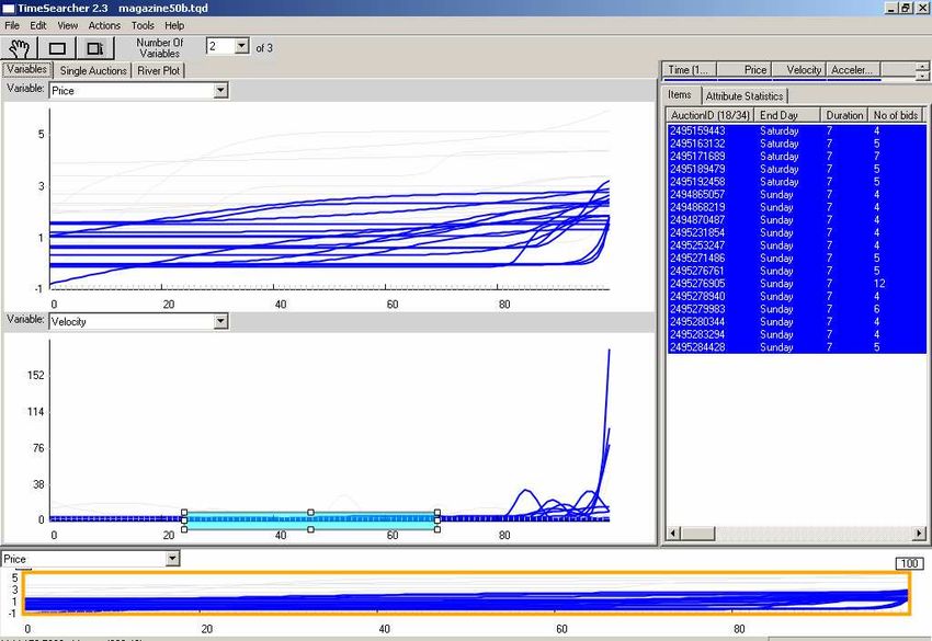
hcil/timesearcher. Figure 11 shows the main screen of the visualization
tool with a dataset of 34 eBay auctions for magazines. The time series are
displayed in the left panel, with 3 series (i.e. 3 variables) for each auction:
“Price” (top), “Velocity” (middle), and “Acceleration” (bottom), which cor-
respond to the price curves and their first and second derivatives, as explained
in the previous section. At the bottom of the screen, an overview of the en-
tire time period covered by the auctions is provided to allow users to specify
time periods of interest to be displayed in more detail on the left panel. On
the right, the attribute panel shows a table of auction attributes. Each row
corresponds to an auction, and each column to an attribute, starting with the
auction ID number. In this dataset there are 21 attributes, scrolling provides
access to attributes that do not fit into the available space. Users can choose
how much screen space is allocated for the different panels by dragging the
separators between the panels, enlarging some panels and reducing others.
All three panels are tightly coupled so that interaction in one of the panels is
immediately reflected in the other panels. Attributes are matched with time
series using the auction ID number as a link.
The interactive visualization operations can be divided into time-series
operations (functional data) and attribute operations . We describe these next.18 Jank, Shmueli, Plaisant, and Shneiderman
Filter Box Search Box Time Series Panel Attribute Panel Variable Number Box
Fig. 11. The main screen of TimeSearcher, showing price curves and dynamics
curves (left) coupled with attribute data (right) for 34 online auctions.
Functional Object Operations
TimeSearcher treats each time-series, represented by a curve, as a single ob-
servation, and allows operations on the complete curve or on subsets of it.
The following operations can be applied to the functional data (curves).
• Curve selection: Selecting a particular curve (or a set of curves) is done
by mouse-clicking on any point in that curve. The selected curve is thenFunctional Visualization 19
highlighted in blue (see Figure 11). Hovering over a curve will highlight it
in orange, thereby simplifying the task of mouse coordination.
• Zooming: The overview panel at the bottom of the screen displays the
time-series for one of the variables and allows users to specify in which
part of the time series they want to zoom in. The orange field of view box
determines the time range that is displayed on the upper left panels. Any
one of the panels can be used for the display in the orange field. To zoom,
users drag the sides of the box. By zooming in, the user can focus on a
specific period in the data and see more details. In many cases zooming also
results in better separation between the curves, enabling easier selection
and un-selection of lines. The box can also be dragged right and left to
pan the display and show a different time period. Regardless of the range
of the detail view, the overview always displays the entire time series and
provides context for the detail view.
• Focusing on a variable: To focus on a certain variable (price, velocity,
or acceleration curves), users can choose to view only that panel on the
left, thereby getting a larger view of those curves. This results in clearer
separation between curves, which can be especially useful when there are
many auctions. Users can specify the number of variables to be shown
(here 1, 2 or 3) and select which of the variables should be displayed. This
allows extra flexibility in the choice of derivatives to display.
• Filtering curves: Users can filter the curves to see only auctions of inter-
est by using filter widgets called TimeBoxes. One can click on the TimeBox
icon of the toolbar and draw a box on the time-series panel of interest.
Every curve that passes through the box (between the bottom and top
edges of the box for the duration that the box occupies) is kept while all
the other curves are filtered by graying-out. The corresponding auctions
are also removed from the attribute panel on the right. Figure 12 shows a
typical filter TimeBox used to see only auctions that end with high price
velocity. In the attributes panel users see that they all ended around the
week-end. They can apply multiple TimeBoxes on the same or separate
variables, which form conjunctive queries (i.e. a combination of the query
of individual TimeBoxes via logical “AND”). For example, users could
search for auctions ending with low prices and with high velocities.
• Searching for patterns in curves: In comparing price curves, and even
more so, price dynamics, a useful tool is the pattern search. This is achieved
by drawing a SearchBox on a selected curve during a certain time duration.
The pattern is the part of the series that the SearchBox horizontally covers,
and it is searched across all other curves not only at the same time but
also at any time point in the auction. There is a tolerance handle on the
right of the SearchBox that allows setting a measure of similarity. For
example, users can search for auctions that have price curves with steep
escalations at any time during the auction. TimeBoxes and SearchBoxes
can be combined into a multi-step interactive search.20 Jank, Shmueli, Plaisant, and Shneiderman
• Functional summaries: One can obtain numerical summaries for a set
of functional objects using the Riverplot in Figure 13. The Riverplot is
a continuous form of the boxplot and displays the (pointwise) median
together with 25% and 75% confidence bounds. The Riverplot allows for a
condensed display of the average behavior of all curves together with the
uncertainty around this average.
Attribute Operations
Manipulating the attribute data, and observing the coupled functional data
is useful for learning about relationships in the data across the different data
types. The following operations support such exploration (in addition to more
standard exploration of attribute data alone).
• Sorting auctions: Users can sort the auctions by any attribute by clicking
on the attribute name in the 1st row. A click sorts in ascending order,
while the next click sorts in descending order. Sorting can be performed
on numerical as well as text attributes. The sorting also recognizes day-
of-week and time formats. The sorting is useful for learning about the
ranges of the values for the different attributes, the existence of outliers,
the absence of certain values, and possible errors and duplications in the
data. Furthermore, sorting might allow users to visually spot patterns of
“similar” auctions, by making auctions with similar values for an attribute
consecutive in the auction list. Users may sort according to more than one
column. In addition, the order of the attribute columns can be changed by
clicking and dragging the attribute names to the right or left.
• Highlighting groups of auctions: After the attribute/s of interest have
been sorted, groups of auctions can be selected and their corresponding
time series in the left panels are highlighted. For example, if the attributes
table is sorted by the end day of the auction, it is easy to select all auctions
that ended on a weekday from the table, and see the corresponding time
series highlighted, revealing that they mostly comprise auctions that end
with the highest prices (Figure 11).
• Summary statistics: The summary statistics tab shows mean, standard
deviation, minimum, max, median, and quartiles for each attribute for the
selected auctions. This is updated interactively when the auctions are fil-
tered with TimeBoxes, or when users select a subset of auctions manually.
For example, while the median seller rating of all auctions is 615, when
users apply a TimeBox to select auctions that started with a low price,
the median seller rating jumps to 1487. Moving the TimeBox to select
auctions that started with a high price results in a median seller rating of
243, which may imply that setting auctions with a low starting price is a
strategy mostly employed by experienced sellers.
The array of interactive operations described above support data explo-
ration and more than that: [Shmueli et al., 2005] describe how these oper-Functional Visualization 21
ations can be used for the purpose of decision making, through a semi-
structured exploration. Exploration can be guided by a set of hypotheses, and
the results can then assist in finding support and directing towards suitable
formal statistical models. In particular, they show how insights gained from
the visual exploration can improve seller, bidder, auction house, and other
vendors understanding of the market, thereby assisting their decision-making
process.
5.2 Forecasting with TimeSearcher
Forecasting the value of a functional object is one field in functional data anal-
ysis that has not received much attention. In forecasting we refer to forecasting
the value of a curve at a particular time t (either a particular curve in the
data or the average curve), based on information contained in the functional
data and the attribute data. We propose a general forecasting procedure as
follows:
1. Selecting similar items: For a partial curve (e.g., an ongoing auction
that has not closed), we select the subset of curves that are closest to the
curve of interest in the sense of similarity in attributes and in the evolution
and dynamics curves. For the attribute criterion, this can be achieved
either by sorting by attributes and selecting items with similar values for
the relevant attributes (e.g., auctions of the same duration and with the
same opening price), or directly by a filtering facility that allows the user
to specify limits on values for each of the attributes of interest (this facility
is currently not available in the public version of TimeSearcher). For the
curve matching, TimeBoxes can be used to find curves that have similar
structure during time-periods of interest (e.g., auctions with high price
velocity on day 1 and high prices on day 3). We are currently working
on developing a facility for “curve matching” that is more automated.
For instance, consider the case of forecasting the closing price of a 7-day
auction that is scheduled to close on a Sunday, with an opening price
of $0.99, and had very low dynamics until now. Let us assume that we
observe this auction until day 6 (85% of the auction duration). Figure 12
illustrates a selection of auctions that all have similar attributes to the
above auction (all 7-day long, with an opening price below $5, and closed
on a weekend), and also share similar curve structure during the first 6
days of the auction (low velocity, as shown by the filtering box placed on
the velocity curves).
2. Forecasting from the similar set: We then use the selected “similar”
set of curves to form a prediction at time t by examining their river plot.
The median at time t is then the forecast of interest, and the quartiles at
that time can serve as a confidence interval. Although this is a very crude
method, it is similar in concept to collaborative filtering. The key is to
have a large enough data set, so that the “similar” subset is large enough.22 Jank, Shmueli, Plaisant, and Shneiderman
To continue our illustration, Figure 13 shows the river plot of the subset
of “similar” auctions. The forecasted closing price is then the median of
the closing prices of the subset of auction, and we can learn about the
variability in these values from the percentile curves on the river plot.
Fig. 12. Filtering the data to find a set of “similar” auctions to an ongoing open
auction.
The forecasting module is still under development, with the goal being a
more automated process. However, the underlying concept is that interactive
visualization can support more advanced operations, even such as forecasting,
compared to static visualization.
6 Further Challenges and Future Directions
Functional data analysis is an area of statistical research that receives grow-
ing amount of interest. To date, most of this interest has centered around
developing new functional models and techniques for their estimation, while
only little effort has been spent on exploratory techniques, and especially vi-
sualization. Classical statistics has received wide-spread popularity not onlyFunctional Visualization 23
Fig. 13. River plot of the subset of “similar” auctions. The thick black line is
the pointwise median that is used for forecasting. The dark gray bands around the
median show the 25 and 75% percentile range and the light gray bands show the
envelope for all similar auctions. This can be seen as a continuous form of box plot.
because of the availability of a wide array of models but also because of the ca-
pability of checking the appropriateness of those models. Only if a researcher
is convinced that a model is appropriate will she wholeheartedly support the
findings from it. Such evidence, however, requires seeing the data in relation
to the model. In that sense, a wide-spread acceptance and usage of functional
models is only going to happen when we have a range of visualization tools
that achieve similar tasks as their counterparts in classical statistics.
In this paper, we have outlined a variety of functional visualizations avail-
able. However, significant challenges remain. These challenges range from con-
currency of functional objects, to high dimensionality, and complex functional
relationships.
6.1 Concurrency of Functional Events
The standard assumption in functional data analysis is independence of the
functional observations in the data set. This assumption may however not24 Jank, Shmueli, Plaisant, and Shneiderman always be plausible. For instance, if the functional object represents the for- mation of price in an online auction then it is quite possible that the price in one auction is affected by that of another one. That is, if the price in one auction jumps unexpectedly high, then this may cause some bidders to leave that auction and move on to another auction for the same item. The result is a dependence in price between the two auctions. Or more generally, the result is a dependence between the two functional objects. It is not straight- forward how this kind of dependence can be captured by a mathematical model. In fact, it is not even obvious how this concurrency can be unveiled in graphical fashion. One promising attempt in that direction is the work of [Hyde et al., 2005] which suggests the use of Rug Plots for the functional objects and their derivatives. 6.2 Dimensionality of Functional Data Another challenge with visualizing functional data is the dimension of the data. As pointed out earlier, it is not uncommon for functional data to be 3-, 4- or even higher-dimensional. Most standard visualization techniques work well for dimension of at most 2, which is the dimension of the paper that we write on and the computer screen that we look at. Moving beyond 2 dimensions is challenging for any kind of visualization task, including that of functional data. 6.3 Complex Functional Relationships In addition to the high dimension, functional data is also often characterized by complex functional relationships. Take for instance the movement of a object through time and space. This movement may be well characterized by a 3- or 4-dimensional differential equation [Ramsay and Silverman, 2002]. However, visualizing a differential equation is not an obvious task. One way is to use phase plane plots like in Figure 5. Other approaches have been proposed in [Schwalbe, 1996]. References [Aris et al., 2005] Aris, A., Shneiderman, B., Plaisant, C., Shmueli, G., and Jank, W. (2005). Representing unevenly-spaced time series data for visualization and interactive exploration. In International Conference on Human Computer Inter- action (INTERACT 2005). [Card et al., 1999] Card, S., Mackinlay, J., and Shneiderman, B. (1999). Readings in Information Visualization: Using Vision to Think. Morgan Kaufmann Publ., San Francisco, CA. [Chen, 2004] Chen, C. (2004). Information Visualization: Beyond the Horizon. Springer Verlag.
Functional Visualization       25

[Cleveland et al., 1996] Cleveland, W. S., Shyu, M., and Becker, R. (1996). The
  visual design and control of trellis display. Journal of Computational and Graphical
  Statistics, 5:123–155.
[Hyde et al., 2005] Hyde, V., Jank, W., and Shmueli, G. (2005). Investigating con-
  currency in online auctions through visualization. Technical report, Smith School
  of Business, University of Maryland.
[Jank and Shmueli, 2005] Jank, W. and Shmueli, G. (2005). Profiling price dynam-
  ics in online auctions using curve clustering. Technical report, Smith School of
  Business, University of Maryland.
[Mills et al., 2005] Mills, K., Norminton, T., and Mills, S. (2005). Visualization of
  network scanning. National Defense and Homeland Security Kickoff Workshop
  of the Statistical and Applied Mathematical Sciences Institute (SAMSI). Poster
  Presentation.
[Plaisant, 2005] Plaisant, C. (2005). Exploring Geovisualization, chapter Informa-
  tion Visualization and the Challenge of Universal Access. Oxford: Elsevier.
[Ramsay and Silverman, 2002] Ramsay, J. O. and Silverman, B. W. (2002). Applied
  functional data analysis: methods and case studies. Springer-Verlag, New York.
[Ruppert et al., 2003] Ruppert, D., Wand, M. P., and Carroll, R. J. (2003). Semi-
  parametric Regression. Cambridge University Press, Cambridge.
[Schwalbe, 1996] Schwalbe, D. (1996). VisualDSolve: Visualizing Differential Equa-
  tions with Mathematica. TELOS/Springer-Verlag.
[Seo and Shneiderman, 2005] Seo, J. and Shneiderman, B. (2005). A rank-by-
  feature framework for interactive exploration of multidimensional data. Infor-
  mation Visualization, 4:99–113.
[Shmueli and Jank, 2005] Shmueli, G. and Jank, W. (2005). Visualizing online auc-
  tions. Journal of Computational and Graphical Statistics, 14(2):299–319.
[Shmueli et al., 2005] Shmueli, G., Jank, W., Aris, A., Plaisant, C., and Shneider-
  man, B. (2005). Exploring auction databases through interactive visualization.
  Decision Support Systems, to appear.
[Shneiderman, 2002] Shneiderman, B. (2002). Inventing discovery tools: Combining
  information visualization with data mining. Information Visualization, 1:5–12.
[Shneiderman and Plaisant, 2004] Shneiderman, B. and Plaisant, C. (2004). De-
  signing the User Interface: Strategies for Effective Human-Computer Interaction:
  Fourth Edition. Addison-Wesley Publ. Co., Reading, MA.
[van Wijk and van Selow, 1999] van Wijk, J. J. and van Selow, E. (1999). Cluster
  and calendar-based visualization of time series data. In Wills, G. and Keim, D.,
  editors, Proceedings 1999 IEEE Symposium on Information Visualization (Info-
  Vis’99), pages 4–9. IEEE Computer Society.
[Wang et al., 2005] Wang, S., Jank, W., and Shmueli, G. (2005). Forecasting ebay’s
  online auction prices using functional data analysis. Technical report, Smith School
  of Business, University of Maryland.
You can also read