Do data from twitter improve predictions of Academy Award winners? - JKU ePUB

Im Diplomstudium Wirtschaftswissenschaften:

 Diplomarbeit zur Erlangung des akademischen Grades Mag.rer.soc.oec

Do data from twitter improve predictions of Academy

 Award winners?

 Klemens Stutzenstein

 Betreut von

 PD René Böheim, PhD

 Johannes Kepler Universität Linz

 Institut für Volkswirtschaftslehre

 Altenberger Straße 69, A-4040 Linz-Auhof, Österreich

 Sankt Georgen an der Gusen, Jänner 2021

Eidesstattliche Erklärung

Ich erkläre an Eides statt, dass ich die vorliegende Diplomarbeit selbstständig und ohne

fremde Hilfe verfasst, andere als die angegebenen Quellen und Hilfsmittel nicht benutzt bzw.

die wörtlich oder sinngemäß entnommenen Stellen als solche kenntlich gemacht habe.

Die vorliegende Diplomarbeit ist mit dem elektronisch übermittelten Textdokument identisch.

Sankt Georgen an der Gusen, 20.01.2021 Unterschrift

 2

Abstract

Users of social media produce an enormous amount of data each day. Before the internet was

an object of everyday life people had to be surveyed to learn their opinion. With the rise of

social media, it became common to post opinions on social media platforms. When people

communicate their opinions before they are asked for it, this increases efficiency. An

automated index could save time and resources that can be better used in other ways. I

analyse if and how data from Twitter can be used to enhance prediction with box office data,

data from Google Trends, and data from Wikipedia. I cannot use the winner from the

Academy Awards directly as I need more than one point in time to compare the Academy

Award winner with my other data sources. Therefore, I substitute the Academy Award winner

with data from a prediction market that focuses on movies, the Hollywood Stock Exchange.

After the computation of my model, I concluded that the variables I generated from Twitter

data are not significant and do not add value for the prediction of Academy Award winners.

 3

Content

 Abstract ........................................................................................................................... 3

List of Figures ..................................................................................................................... 8
1. Introduction ................................................................................................................. 9
2. Literature Review....................................................................................................... 10
 2.1. Prediction Markets ............................................................................................... 11

 2.1.1.1. Hollywood Stock Exchange (HSX) ............................................................ 12

 2.1.1.2. Are prediction markets good at predicting future outcomes? ....................... 13

 2.2. Social Media........................................................................................................ 14

 2.2.1. Twitter ............................................................................................................. 17

3. Econometric Model and Variables .............................................................................. 17
 3.1. Underlying Hypotheses ........................................................................................ 19

 3.1.1.1. Hypothesis 1: The HSX price correlates with a movie’s success at the
 Academy Awards. ...................................................................................................... 19

 3.1.1.2. Hypothesis 2 and 3: The index and volume of tweets about a certain
 movie/actor/actress/director correlate with success at the Academy Awards. ................ 20

 3.1.1.3. Hypothesis 4: Commercial Success leads to Artistic Success....................... 21

 3.1.1.4. Hypothesis 5: If more people navigate to a movie’s Wikipedia page it is more
 likely that it wins one or more Academy Awards......................................................... 22

 3.1.1.5. Hypothesis 6: If more people search for a movie on Google it is more likely
 that it wins one or more Academy Awards. ................................................................. 23

 3.2. Data .................................................................................................................... 23

 3.2.1.1. Twitter Data .............................................................................................. 23

 3.2.1.2. Volume of tweets ...................................................................................... 23

 3.2.1.3. Index of tweets .......................................................................................... 25

 3.2.1.4. HSX Data – dependent variable ................................................................. 27

 3.2.1.5. Box Office Data ........................................................................................ 28

 3.2.1.6. Wikipedia data .......................................................................................... 32

 3.2.1.7. Google Trends data.................................................................................... 33
 4

4. Descriptive statistics ................................................................................................ 34

4.1. Summary statistics ............................................................................................... 34

4.2. Variable Specification .......................................................................................... 35

4.3. Correlation .......................................................................................................... 37

5. Panel Data Models .................................................................................................. 41

5.1. Variables ............................................................................................................. 41

5.2. Regression estimators .......................................................................................... 44

 5.2.1. Pooled OLS (Ordinary Least Square)............................................................. 44

 5.2.2. Panel models................................................................................................. 44

 5.2.2.1. Fixed effects (FE) ...................................................................................... 44

 5.2.2.2. Random Effects (RE)................................................................................. 45

 5.2.2.3. Swamy-Arora (SA).................................................................................... 45

5.3. Tests for model selection ...................................................................................... 45

5.3.1. Hausman test .................................................................................................... 45

5.3.2. F-Test .............................................................................................................. 46

5.4. Panel data estimation method ............................................................................... 46

5.5. Possible Problems with Endogeneity .................................................................... 46

5.5.1. Solution ........................................................................................................... 47

5.5.2. Testing for Endogeneity.................................................................................... 48

6. Estimation results .................................................................................................... 49

6.1. Comparison table ................................................................................................. 49

6.2. OLS regression .................................................................................................... 50

6.3. Fixed effects regression ........................................................................................ 50

6.4. Random effects regression ................................................................................... 50

6.5. Swamy-Arora regression ...................................................................................... 51

6.6. Tests for model selection ...................................................................................... 51

 6.6.1.1. Hausman test for FE vs. RE ....................................................................... 51

 6.6.1.2. F-Test for FE vs. OLS ............................................................................... 52
 5

6.7. Results ................................................................................................................ 52

 6.8. Prediction ............................................................................................................ 53

 6.8.1. Correct Predictions (in-sample) ..................................................................... 53

 6.8.1. Correct Predictions (out-of-sample) ............................................................... 54

 6.9. Comparison to the literature ................................................................................. 54

7. Conclusio................................................................................................................... 55
 7.1. Further research ................................................................................................... 56

 7.2. Limitations .......................................................................................................... 56

8. Appendix ................................................................................................................... 57
 8.1. Data .................................................................................................................... 57

 8.2. Histograms and Q-Q plots of independent variables .............................................. 59

 8.2.1.1. Twitter volume .......................................................................................... 59

 8.2.1.2. Twitter index ............................................................................................. 60

 8.2.1.3. US weekend receipts ................................................................................. 61

 8.2.1.4. US weekend average receipts ..................................................................... 62

 8.2.1.5. US weekend rank ...................................................................................... 63

 8.2.1.6. US weekend number of screens.................................................................. 64

 8.2.1.7. Google Trends ........................................................................................... 65

 8.2.1.8. Wikipedia.................................................................................................. 66

 8.3. Correlation tables ................................................................................................. 67

 8.3.1.1. Independent variable – dependent variable ................................................. 67

 8.3.1.2. Dependent variable – dependent variable.................................................... 68

 8.1. Variation ............................................................................................................. 70

 8.2. Estimation tables.................................................................................................. 71

 8.2.1. OLS regression................................................................................................. 71

 8.2.2. Fixed effects regression .................................................................................... 72

 8.2.3. Random effects regression ................................................................................ 73

 8.2.4. Swamy-Arora regression .................................................................................. 74
 6

8.3. F-Test for FE vs. OLS .......................................................................................... 74

Bibliography ..................................................................................................................... 75

 7

List of Figures

Figure 1: Underlying Hypotheses ....................................................................................... 19
Figure 2: Accuracy of the HSX award options market. ....................................................... 20
Figure 3: Comparison between movies in million USD ....................................................... 22
Figure 4: Advantages and weaknesses of different Twitter data sources ............................... 26
Figure 5: US weekend receipts example for "American Sniper" in US Dollars. .................... 29
Figure 6: US weekend receipts for all movies in US Dollar. ................................................ 30
Figure 7: weekend average receipts example for "American Sniper" ................................... 31
Figure 8: weekend rank example for "American Sniper" ..................................................... 31
Figure 9: weekend number of screens example for "American Sniper" ................................ 32
Figure 10: Wikipedia hits per day example for "American Sniper" ...................................... 33
Figure 11: Google Trends data for "Gravity","Her","Nebraska","Philomena" and "Frozen".. 34
Figure 12: Summary statistics ............................................................................................ 34
Figure 13: histogram of "HSX" .......................................................................................... 36
Figure 14: histogram of "log of HSX" ................................................................................ 36
Figure 15: Q-Q plot of "HSX" ............................................................................................ 37
Figure 16: Q-Q plot of "log of HSX" .................................................................................. 37
Figure 17: Correlation table for all variables ....................................................................... 38
Figure 18: Twoway linear prediction plot “log of HSX” and “log of Twitter volume” .......... 39
Figure 19: Two-way linear prediction plot “log of HSX” and “log of Twitter index” ........... 40
Figure 20: Comparison of OLS, fixed effects, random effects, and Swamy-Arora models. ... 49
Figure 21: Comparison of in-sample predictions with and without twitter data…………….. 53
Figure 22: Comparison of out-of-sample predictions with and without twitter data…………54

 8

1. Introduction

I analyse if social media data from Twitter will enhance predictions with data from the Box

Office, Google Trends and Wikipedia. Prediction markets such as the Hollywood Stock

Exchange or the Iowa Electronic Market generate forecasts for different kinds of settings. A

major disadvantage of using prediction markets for forecasting is that they are costly, demand

time to be set up, and need enough participants to generate valuable forecasts. I analyse if data

from Twitter in combination with the above-mentioned sources outperform predictions from

the Hollywood Stock Exchange.

The current price for a certain product on a given market offers a good indicator about the future

price (Putler 1992, 287). For settings with no actual markets researchers started “prediction

markets”. The first was the IEM, the Iowa Electronic Market (Berg and Rietz 2006, 142). In

these markets people bet on the outcome of a certain event (Berg and Rietz 2006a, 1). Since the

start of the IEM in 1988, prediction markets proved to be accurate in predicting future events

(Berg and Rietz 2006, 142), (Berg and Rietz 2006a, 12). For predicting another interesting, yet

not thoroughly researched method arose: the use of social media data. Large amounts of data

are generated every day. Making use of these data could bring significant benefits. Being able

to predict the winner of an Academy Award category is of economical relevance as it would

allow people to bet on the winner and make money (if the prediction model is better than the

betting market). The use of an (half) automated index increases efficiency, as it saves resources

that could be better used in other ways. Kogan et al. (2020) propose an early-warning system

for COVID-19 tracking using six digital data sources: (1) COVID-19-related search terms with

Google Trends, (2) COVID-19-related tweets, (3) searches from UpToDate (a search data base

with clinical knowledge used by physicians around the world) that are COVID-19-related, (4)

predictions by GLEAM (Global Epidemic and Mobility Model – an epidemic model that tracks

 9

global disease spread), (5) human mobility data from smartphones and (6) Smart Thermometer

measurements from Kinsa. Kogan et al. found that Twitter data showed significant growth 2-3

weeks, before the growth was visible in confirmed cases. Their combined model was able to

predate an increase in COVID-19 cases with a median of 19.5 days. This information could be

valuable for politicians who must decide when stricter or less strict regulation have to be taken.

During the economic crisis that started in 2008 Askitas and Zimmermann (2009) researched an

innovative method for predicting unemployment in Germany. They performed searches on

Google Insights (later renamed to Google Trends) using two clusters of keywords. The first

cluster contains “Arbeitsamt” or “Arbeitsagentur” and the second cluster contains popular job

search engines in Germany. The prediction matches the unemployment rate closely (R² = 0.909)

and offers the benefit that it is available two weeks before the official unemployment rate is

released.

I use data from the Hollywood Stock Exchange (HSX), box office data, data from Twitter,

Google Trends, and Wikipedia. The left-hand side variable is taken from data from the HSX

which I use as an indicator for the Academy Award winner. The right-hand side consists of

variables from box office, Twitter, Google Trends, and Wikipedia data. I compare pooled

OLS with fixed effects and random effects models to analyse which model is consistent with

my data. After performing tests for model selection, I choose a fixed effects model.

2. Literature Review

Some speculative markets offer good predictions of future events indicated by the price of a

share. Aggregated trader information captures the probability of future events (Bothos,

Apostolou and Mentzas 2010, 50). Depending on the accuracy of the traders’ beliefs every

single trader generates more or less money (Bothos, Apostolou and Mentzas 2010, 51, Zitzewitz

 10

2004, 2). Markets are not available for every kind of information. For some purposes, that are

not covered by “thick“ markets, prediction markets arose. An example for a prediction market

is the Hollywood Stock Exchange (HSX). The HSX allows people to trade shares of different

movies in the fictional currency “Hollywood Dollar” (H$).

 2.1. Prediction Markets

The first real-money prediction market - also known as “information market”, “idea futures”,

“decision markets” or “event futures” - (Zitzewitz 2004, 108, Zhao, Wagner and Chen 2008,

285) was founded in 1988 and is called the Iowa Electronic Market (Berg and Rietz 2006, 142).

Built to forecast presidential elections, the IEM expanded to predict other events in 1993 (J. N.

Berg 2003, 1). Throughout the years, the IEM proved itself to be quite accurate in forecasting

political elections, box office revenues, financial outcomes for companies, etc. (J. N. Berg 2003,

1, Berg and Rietz 2006a, 142-149). Besides the IEM, several other prediction markets arose.

For this study, the Hollywood Stock Exchange (www.hsx.com), founded in 1996 and focusing

on box office records and Academy Awards, serves as independent variable (J. N. Berg 2003,

3, Hollywood Stock Exchange 2010). Contrary to the IEM, the HSX trades fictional shares

bought through Hollywood Dollars (Levmore 2003, 592). The HSX is said to be the gold

standard of predictions in the movie industry (Schoen, et al. 2013, 539).

Due to the fact that in prediction markets participants trade contracts of events happening in the

future trying to maximize their output and aggregate their information, prices in prediction

markets should reflect the likelihood of future events (Zitzewitz 2004, 108, Wolfers J. 2006,

2, J. N. Berg 2003, 3, Bothos, Apostolou and Mentzas 2010, 50).

 11

2.1.1.1. Hollywood Stock Exchange (HSX)

On the Hollywood Stock Exchange participants get H$ (Hollywood Dollars) 2,000,000 for

opening an account (Hollywood Stock Exchange 2014). With this virtual money derivatives of

Hollywood movies can be bought: MovieStocks focus on domestic box office (Hollywood

Stock Exchange 2017), Celebstock are issued for celebrities in different field of entertainment

(Hollywood Stock Exchange 2017), TVStocks cover TV series (Hollywood Stock Exchange

2017) and AwardOptions focus on Academy Award nominees (Hollywood Stock Exchange

2018).

The winner of an “AwardOption” will get approximately H$25 per option while all others delist

at H$ 0.00. The combined “AwardOptions” for one category sum up to H$25 on day one of

trading. The higher the price for one option (one film, actor/actress or director), the higher

should the expected probability of this option be to win the category. The AwardOption halt

trading at 1 p.m. Pacific Standard Time on the day of the Academy Award ceremony

(Hollywood Stock Exchange 2014).

HSX AwardOptions are traded in the following eight categories (Hollywood Stock Exchange

2014):

 1. Best Picture: 5-10 movies depending on the year

 2. Best Director: 5 directors

 3. Best Actor: 5 actors

 4. Best Actress: 5 actresses

 5. Best Supporting Actor: 5 actors

 6. Best Supporting Actress: 5 actresses

 7. Best Adapted Screenplay: 5 movies

 8. Best Original Screenplay: 5 movies

 12

2.1.1.2. Are prediction markets good at predicting future

 outcomes?

Former studies show that prediction markets are good predictors of future events. Spann and

Skiera (2009) test prediction markets versus betting odds and tipsters. They conclude that

betting odds and prediction markets perform equally well when using data from three seasons

of the German premier soccer league and both outperform tipsters. Levmore (2003) analysed

data from the Iowa Electronic Market (IEM) and the HSX. He shows that the averaged error

rate on IEM is 1.37% for the last four elections. At the same time the Wall Street Journal polled

members of the Academy of Motion Arts and Sciences for the six major category winners of

the Academy Award. While this poll predicted five out of six winners right, the HSX predicted

eight out of eight winners right (Wall Street Journal did not poll the winners for best supporting

actor and best supporting actress). Leigh and Wolfers (2006) review the efficacy of polls

(ACNielsen, Galaxy, Morgan and Newspoll) compared to prediction markets (BetFair and

Centrebet) for the election 2004 in Australia. They compare three forecasting horizons: 1 year

prior to the election, 3 months prior to the election and the election eve. Both prediction markets

forecasted the right winner in all 3 forecasting horizons. One year prior to the election only one

out of four polls forecasted the right winner. The same is true for 3 months before the election.

On election eve two out of four polls forecasted the right winner. Leigh and Wolfers show that

prediction markets performed substantially better than pollsters for the 2004 Australian

elections. Pennock et al. (2001) extract probabilistic forecasts for three “online games” – the

HSX, the Foresight Exchange (FX) and the Formula One Pick Six (F1P6) competition. When

evaluating box office forecasts, they use a model that combines data from the HSX with

forecasts from the movie expert Brandon Gray from Box Office Mojo. They collected data from

50 movie openings between March 3, 2000 and September 1, 2000. Their model correlates with

box office revenue at 0.956. Pennock et al. also assessed the HSX “AwardOption” for the 2000

 13

Academy Awards. They compared the HSX prices to expert opinions of five columnists of the

“Hollywood Stock Brokerage and Resource”, a fan site of HSX. From the opening of the

“AwardOption” market on February 15, 2000 to the market close on March 26, 2000, the HSX

score increased almost continuously. By February 19, 2000 the HSX score surpassed all five

experts.

Prediction markets do have several limitations. People tend to underestimate large probabilities

and overestimate small probabilities. This may lead to an inefficient market (Zitzewitz 2004,

120). If there is an advantage to gain, people might try to manipulate the prediction market –

depending on how thin the prediction market is (Zitzewitz 2004, 123). Also, participants might

not trade based on objective probabilities, but on personal desires and interests, thus leading to

inefficient markets (Bothos, Apostolou and Mentzas 2010, 51).

 2.2. Social Media

Social media changes the way we communicate with each other (Qualman 2013, 5-12). People

exchange opinions, impressions and experiences, they generate and share content (Hilker 2010,

11, Kalampokis, Tambouris and Tarabanis 2013, 454). This transforms the consumer to a

“prosumer” who does not only consume information but also generates part of it (Kaplan 2010,

66).

The use of social media may offer a new source for researchers (Lu, Wang and Maciejewski

2014, 58). Data in social media are generated at a high frequency, therefore enabling predictions

that cannot be realized with traditional surveys or administrative resources (D. C. Antenucci

2014, 1-2). Furthermore, social media data can often be generated at lower costs than traditional

sources (D. C. Antenucci 2014, 2, Bothos, Apostolou and Mentzas 2010). Another advantage

of social media data is that they carry incremental information that cannot be generated using a
 14

prediction market (D. C. Antenucci 2014, 4, Diakopoulus and Shamma 2010, 1198).While

prediction markets react to events – the events that cause changes in prediction markets

themselves remain unclear. Twitter data offer a possibility to identify events that cause

movements in prediction market graphs. These events are often marked with hashtags: “#”.

Disadvantages of social media are that the data are not structured and are not gathered for a

special purpose (like data from the HSX). Another detrimental effect is that manipulation might

occur if there are enough incentives for doing so. Most likely, Twitter data are biased because

younger people and people from urban areas are overrepresented (Gayo-Avello 2011, 122;128).

Also, users on the internet tend to express extreme positive or negative experiences more often

than moderate experiences (Yu and Kak 2012). Furthermore, raw social media data are very

noisy and need substantial effort to be transformed into high quality data that can be used for

statistical analysis (Kalampokis, Tambouris and Tarabanis 2013, 545). According to Schoen et

al. (2013), prediction markets and social media data cannot be compared as in prediction

markets people put their (virtual) money on the participant they think will win. In social media

people give mentions. That does not necessarily have to reflect their opinion.

Sheng Yu and Subhash Kak identify three requirements for predicting with social media (Yu

and Kak 2012):

 - The event to predict must be human related: non-human-related events, for example the

 development of an eclipse, has nothing to do with social media data and therefore cannot

 be predicted.

 - Masses of people must be involved: they act as a sample but might have a built-in bias

 (not everyone is posting his/her opinion on social media).

 15

- The event to predict must be easy to be talked about in public: topics that are affected

 by social pressure will lead to biased predictions.

Using social media data for predicting the Academy Award winners seems perfect for

conducting a study about.

Several studies cover the topic of user generated data for the prediction of certain events:

Desai et al. (2012) use Google internet query share data with keywords like “stomach virus”,

“stomach flu”, “stomach illness”, “stomach bug”, “stomach sickness”, and “stomach sick” and

construct a model that they compare to US norovirus outbreak surveillance data. Their model

shows a strong correlation (R²=0.95). Tumasjan et al. (2010) show that using the mere number

of tweets about political parties, the share of tweets comes close to traditional election polls

(MAE: 1,65%). A downside of this study is that they look at one election only, so they do not

use a sophisticated data base. Antenucci et al. (2014) create indexes of job loss using tweets

containing keywords that are associated with job loss (“axed”, “canned”, “downsized”,

“outsourced”, “pink slip”, “lost job”, “fired job”, “been fired”, “laid off”, “uneployment”) and

close variants. Their index tracks initial claims for unemployment insurance and predicts 15-

20% of the variance of the prediction error of the consensus forecast for initial claims.

Antenucci et al. also created a website for the so-called “University of Michigan Social Media

Job Loss Index” (Antenucci, Shapiro and Cafarella 2017). It was last updated in 2017 and offers

a download for all initial claims and predictions from 2011-2017. While the average weekly

deviation from the initial claims was 2.86% in 2011, it increased to 4.29% in 2012, 6.76% in

2013, 14.97% in 2014, 25.16% in 2015, 21.81% in 2016 and 15.81% in 2017 (until mid-July).

Asur and Huberman (2010) compare HSX data with a tweet rate time series to predict box

office revenues for 24 different movies. They show that R² for their Twitter time series (0.973)

is slightly better than R² for the HSX time series (0.965).

 16

Thelwall, Buckley and Paltoglou (2011) assess if popular events lead to an increase in sentiment

strength. They study the most popular events within a month of English tweets and measure the

most popular events with a relative increase in term usage. It is surprising for the authors that

negative sentiments play a much bigger role than positive sentiments. They test three

hypotheses on negative sentiments that all deliver strong evidence at a 1% level. Out of the

three hypotheses on positive sentiments two were not significant and one was significant at a

5% level. To the authors it seems that people express their opinions on Twitter and that these

posts are more negative than average for the topic. Their main finding is that important events

on Twitter are associated with increases in average negative sentiment strength.

 2.2.1. Twitter

Twitter is the biggest microblogging platform. A microblog (tweet) was initially a short

message of up to 140 (since September 26, 2017 280) characters (Isaac 2017). In 2019, Twitter

had 321 million monthly active users (Statista Inc 2019) who generated 500 million tweets a

day (Twitter Inc. 2019). People communicate about their lives (D. C. Antenucci 2014, 5) and

share thoughts, opinions, and behaviour on Twitter (Kalampokis, Tambouris and Tarabanis

2013, 554).

3. Econometric Model and Variables

I analyse if a model that contains Twitter data can predict the winners of Academy Awards

between 2009 and 2015 better than the same model without Twitter data.

I focus on the usefulness of user generated data from Twitter in combination with common

market data (US weekend receipts, US weekend average receipts per screen, US weekend rank,

 17

US weekend number of screens), hits on the English version of a movie’s Wikipedia page,

Google Trends data and compared to the prediction market “Hollywood Stock Exchange”.

I assume that a movie that gets a lot of mentions from users on Twitter is more likely to win an

Academy Award than a movie that gets only little feedback. I do, however, not state that

mentions on Twitter directly influence the opinions of members of the Academy of Motion

Picture Arts and Sciences. I only assume that artistically good movies get more mentions and

are also more likely to win an Academy Award. According to Tumasjan et al. the number of

tweets without implementing any sentiment analysis represents a plausible prediction

(Tumasjan, et al. 2010, 183). Asur and Huberman show that the rate of tweets per day explained

about 80% of variance in movie revenue prediction (Asur and Huberman 2010, 495).

 18

3.1. Underlying Hypotheses

Figure 1: Underlying Hypotheses

Figure 1 lists the underlying hypothesis, from H1 to H6. While there is enough evidence for

H1-H4, studies that test H5 and H6 are rare.

 3.1.1.1. Hypothesis 1: The HSX price correlates with a movie’s

 success at the Academy Awards.

Chen and Krakovsky (2010) state that the accuracy of the Hollywood Stock Exchange is

remarkably high and beats critics in most years. Pennock, Nielsen and Giles (2001) show that

HSX prices are more accurate than expert opinions in predicting the winners of the Academy

Awards. Pennock et al. (2001) state that HSX prices correlate well with actual award outcome

frequencies (see graph below).

 19

Figure 2: Accuracy of the HSX award options market. Points show frequency versus average normalized price for
buckets of similarly priced options. The dashed line indicates perfect accuracy - figure from (Pennock, Nielsen and
Giles 2001, 179)

 3.1.1.2. Hypothesis 2 and 3: The index and volume of tweets

 about a certain movie/actor/actress/director correlate with

 success at the Academy Awards.

Movies are experience goods – you must see one, before you are sure you like it. To decide if

you want to see a movie therefore depends on the perceived quality (Deuchert, Adjamah and

Pauly 2005, 159). One of the most important quality signals is word of mouth, which spreads

faster the larger the user base is (Deuchert, Adjamah and Pauly 2005, 160). Another quality

signal is user ratings. Bothos, Apostolou and Mentzas (2010) investigate the correlation

between user ratings and the Academy Award winners but could not find statistically

significant predictors. The third important quality signal, the review of critics, is investigated
 20

by Reinstein and Snyder (2005). They used reviews from two popular movie critics (Siskel

and Ebert) to analyse if their reviews have a detectable effect at the box office. They conclude

that positive reviews (2 thumbs up) have a small effect in magnitude (25%) but are only

marginally statistically significant.

Ravid (1999) tests a sample of 180 films released between late 1991 and early 1993. He

creates three different indexes that contain reviews. Index1 = positive reviews/total reviews,

Index2 = (positive reviews + neutral reviews)/total reviews and Index4 = total number of

reviews. Only Index4 is significant at a 1% level and thus he finds evidence that the more

reviews a movie gets, the more economically successful it is – irrespective of whether they

are positive or not.

 3.1.1.3. Hypothesis 4: Commercial Success leads to Artistic

 Success.

While there is enough evidence for artistic success leading to commercial success, studies,

investigating the opposite relationship, are rare. The Economist, for example, stated in 1995

that winning the main category “best picture” increased box office receipts by $25 million

(The Economist 1995, 92).Terry et al. (2005) conclude that an Academy Award nomination

leads to a six million dollar increase in domestic (US) revenue.

Hadida (2010) explicitly tests the hypothesis that the more commercially successful a film is,

the higher its artistic recognition is. She does not reject this hypothesis (0.150, p < .001)

(Hadida 2010, 66).

According to Deuchert et al. (2005) higher quality movies might pull more people into the

cinemas. The following table by Deuchert et al. combined with the information that movies

make between 30.81% (own calculation with data from boxofficemojo.com) and 34% (Terry,

 21

DeArmond and Zachary 2009, 177) of their domestic (US) revenue on the opening weekend

makes it reasonable to believe that a higher grossing movie is more likely to win an Academy

Award (Deuchert, Adjamah and Pauly 2005).

Figure 3: Comparison between movies, Academy Award nominated movies and Academy Award winner movies in
million USD

 Average total US

 box office revenue
 Average US running
 (in million USD)
 time (weeks)

 All movies 25.48 (41.41) 16.08 (9.96)

 Only nominated 41.90 (50.08) 24.01 (10.77)

 Winner movies 90.55 (107.54) 35.20 (12.28)

 Note. Standard deviations are given in parentheses. Deuchert et al. (2005) show that the average box office revenue in

 million USD of all movies in their study is 25.48. They use the 204 most successful movies of each year between 1990 and

 2000. When looking at Academy Award nominated movies only the average box office return in million USD increases to

 41.90. The last column shows only the Academy Award winner movies with an average box office return of 90.55 million

 USD.

 3.1.1.4. Hypothesis 5: If more people navigate to a movie’s

 Wikipedia page it is more likely that it wins one or more

 Academy Awards.

There are hardly any studies that investigate the relationship between Wikipedia hits and

movie performance. Mestyàn, Yasseri and Kertész (2013) published a study that contains a

prediction model based solely on Wikipedia data that was able to predict box office movie

success a month prior to movie release with an R2 coefficient of 0.77.

 22

3.1.1.5. Hypothesis 6: If more people search for a movie on

 Google it is more likely that it wins one or more Academy

 Awards.

For assumption number 6 the same is true as for assumption 5. A simple regression model of

Yahoo!’s Web search query logs for the US market correlates strongly (0.85) with actual

revenue of 119 feature films between October 2008 and September 2009 (Goel, et al. 2010,

17487).

 3.2. Data

 3.2.1.1. Twitter Data

I use a dataset that consists of tweets about movies, actors and directors of 117 Academy

Award-nominated films between 2009 and 2015. These data include 306,016 tweets.

Data from Twitter are gathered using Twitter’s advanced search feature. I create two

variables: number of tweets and an index created based on positive, negative and neutral

mentions.

 3.2.1.2. Volume of tweets

Every tweet that fulfils the requirements of a predefined query is displayed on Twitter’s

advanced search. One query defines a film, actor/actress or director people talk about. Here is

an example of a query for a film:

“Name of film/director/actor” “Oscar” “lang:en” “since:YYYY-MM-DD until:YYYY-MM-

DD” (Y stands for year, M for month and D for day). The variable “Volume of tweets”

 23

represents the number of tweets (normalized to 1 for each category) about a certain

actor/director/film.

“Lang:en” means that only English tweets are gathered and “Since” and “Until” mark the time

frame that data are gathered for (Twitter’s advanced search does not offer the possibility to

segment after geographical data, so I segment tweets based on language).

For the movie “American Sniper” a query looks as follows:

American Sniper oscar lang:en since:2015-01-24 until:2015-02-22

The data are collected for each day and are then aggregated to weekly data to make them

comparable. In the next step, all tweets per week in each category are added up to “total

tweets per category”. This number is important to make the data comparable. In the categories

“best picture” and “best actor/actress” the number of tweets is much higher than in “best

director” or “best supporting actor/actress”. If I do not account for this the latter categories are

underrepresented. After this transformation, the tweets per movie/director/actor/actress in

each category always add up to one.

The reason for including the volume of tweets into my panel data set is that some studies

suggest that the number of tweets/opinions correlates significantly with different output data –

for example HSX (Doshi 2010, 44) or elections (Tumasjan, et al. 2010, 184). I do not think

that the number of mentions will provide very useful data. If there are a lot of mentions, but

all are negative I do not think this number will be correlated with winning an Academy

Award.

 24

3.2.1.3. Index of tweets

I create an index consisting of the number of positive mentions, the number of negative

mentions and the number of all mentions. The formula for the index looks as follows:
 _ − _ 
 _ = _ 
 where “Twitter Index” ( _ )is the index for a

movie/actor/actress/director (x) at time (t), m_pos is the number of positive mentions for a

movie/actor/actress/director (x) at time (t), m_neg is the number of negative mentions for a

movie/actor/actress/director (x) at time (t) and m_all is the number of mentions for a

movie/actor/actress/director (x) at time (t).

The query for m_pos: Name of film/director/actor/actress win Oscar lang:en since:YYYY-

MM-DD until:YYYY-MM-DD

The query for m_neg: Name of film/director/actor/actress win Oscar cannot OR can't OR

"should not" OR shouldn't OR "will not" OR won't OR "might not" OR don't lang:en

since:YYYY-MM-DD until:YYYY-MM-DD

The query from m_all: Name of film/director/actor/actress Oscar lang:en since:YYYY-MM-

DD until:YYYY-MM-DD

Sentiment-based analysis is quite en-vogue, although it is difficult for computers to

understand the meaning of human communication. It is difficult for programs to assign the

right sentiment if the communication is short. Therefore, automatic sentiment analysis is

difficult for tweets.

Sentiment Analysis is questioned by some (Gayo-Avello 2011, 128), especially widely used

automatic sentiment analysis software. Metaxas et. al (2011) show that the accuracy of

sentiment analysis software is only slightly better than a random classifier assigning positive,

negative and neutral sentiments. When they investigate a smearing campaign against a

 25

candidate to the US Senate, more than a third of the contained tweets were tagged as positive

mentions.

Advantages and Weaknesses of different Twitter data sources

For collecting data from Twitter there are 4 different approaches:

Twitter Advanced Search: Twitter’s own search engine. All tweets since 2009 are

accessible.

Twitter Data Grants: Twitter started a pilot program for selected academic institutions in

2014 (Krikorian 2014). It seems this program has either ended or is not promoted anymore.

Twitter API: Twitter’s application programming interface allows people to export tweets

after defining a query.

Third Party Programs: social media monitoring programs often offer a Twitter

implementation that gathers data in real time. Most of these programs also offer a sentiment

analysis part.

Figure 4: Advantages and weaknesses of different Twitter data sources

 Advantage Weakness

 Twitter Advanced • free • no export function of

 Search • full data set tweets

 • reliable

 Twitter Data Grants • free • not accessible

 • full data set

 • reliable

 • export function

 26

Twitter API • free • historical data only for

 • export possibility the last 2 weeks

 • requires coding skills

 Third Party Programs • user friendly • expensive

 • often contain sentiment • a query must be defined

 analysis software before being able to

 gather data

 3.2.1.4. HSX Data – dependent variable

As HSX “AwardOption” data are publicly available only for the current Academy Award

ceremony, I bought a dataset (2009-2015), which consists of the aggregated price for each

option (movie/actor/actress/director) in the main 8 categories for every day from at least 4

weeks before the Academy Award ceremony from the Hollywood Stock Exchange. Each year

approximately four to six weeks before the Academy Award ceremony, the HSX starts its

“AwardOption” where people buy and sell options of Academy Award-nominated movies.
 25
The starting price is H$ for each movie in the main category “best picture”
 
(8 nominees in 2015 – the number of nominees in the main category ranges from 5 to 10

depending on the year) and 5 H$ for the other 7 categories (5 nominees each). The

“AwardOption” closes on Sunday, 1 p.m. Pacific Standard Time right before the Academy

Award ceremony. Options can be traded at any time.

 27

3.2.1.5. Box Office Data

This dataset contains all Academy Award nominated movies in the main 8 categories for the

years 2009-2015. The data are gathered from “Wolfram Alpha” (See

https://www.wolframalpha.com or appendix for more information) and consist of “US weekend

receipts”, “US weekend average receipts per screen”, “US weekend rank”, and “US weekend

numbers of screens”.

As the Hollywood Stock Exchange only covers eight different categories (best director, best

supporting actor, best supporting actress, best picture, best original screenplay, best actor, best

actress and best adapted screenplay), I lose some information about the movies that are not

covered. As HSX prices are the dependent variable there is no other way than to drop the data

from movies that are not covered by the HSX.

US weekend receipts

US weekend receipts are measured in 100,000 US Dollars (inflation adjusted to May 2016 US

Dollars) in line with earlier studies by Robins (1993), Miller and Shamsie (2001) and Nelson,

Donihue and Waldman (2001) about the movie industry. In line with Bothos, Apostolou and

Mentzas (2010), I include the first four weeks after the wide opening of a movie. According to

Deuchert et al. this is acceptable as they find a positive and significant impact of the first week’s

box office revenues on the weekly revenues of the following weeks. Nevertheless, movies do

not automatically generate financial success if the first week was successful (Deuchert,

Adjamah and Pauly 2005, 172).

 28

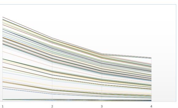
The example below shows US weekend receipts for “American Sniper”:

Figure 5: US weekend receipts example for "American Sniper" in US Dollars January to June 2015.

The graph for weekend receipts looks similar for most of the movies. Movies tend to generate

the biggest revenue in week one after wide release. In this graph wide release is in mid-

January. The low amplitude before mid-January is the limited release in a few selected

cinemas.

 29

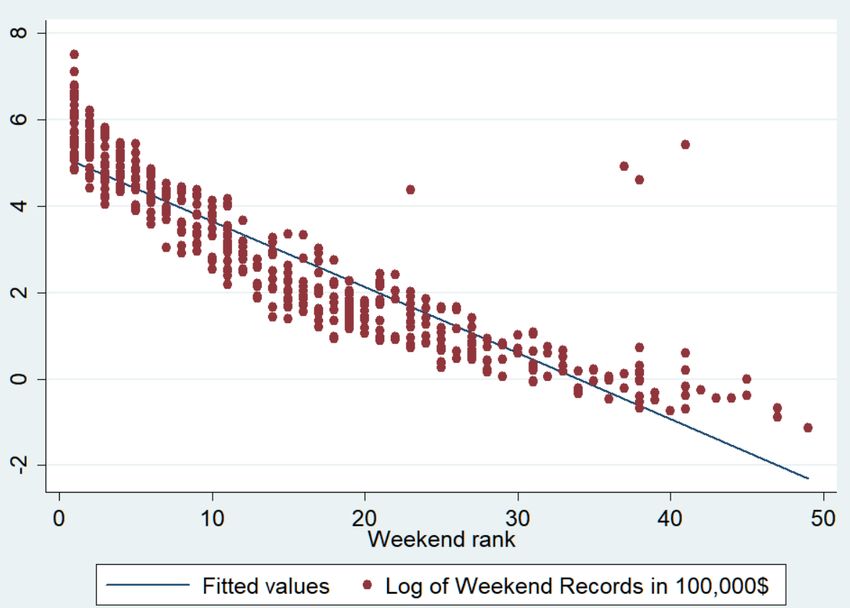
Figure 6: US weekend receipts for all movies in US Dollar.

This graph shows the aggregated receipts per week of all movies in US-Dollars. It clearly

shows that the biggest revenue is generated in the first week after wide release and then

declines over time. The x-axis marks weeks since wide release.

US weekend average receipts per screen

US weekend receipts are measured in 1,000 US Dollars, inflation adjusted to May 2016 US

Dollars. The example below shows the US weekend average receipts per screen for

“American Sniper”.

 30

Figure 7: weekend average receipts example for "American Sniper"

This graph again shows the limited release phenomenon. Until mid-January the film is only

released in a few selected cinemas. According to the average receipts per screen the limited-

release cinema shows attract a lot more viewers per screen than the shows after wide release.

weekend rank

Figure 8: weekend rank example for "American Sniper"

The same is true for “weekend rank”. During the limited release the movie ranks low on

cinema charts. This is comprehensible as the movie is only shown in a few selected cinemas.

 31

When “American Sniper” releases to a wide audience it instantly ranks first on the “weekend

rank” chart.

weekend number of screens

Figure 9: weekend number of screens example for "American Sniper"

In the beginning of January, the movie runs only on a few screens (limited release).

Therefore, the weekend receipts are low, the average receipts per screen are high and the

weekend rank is low until wide release.

 3.2.1.6. Wikipedia data

Wikipedia data are measured in hits per day on the English version of the Wikipedia page

about the film, actor, actress or director and are then aggregated to a weekly average.

 32

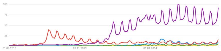
Figure 10: Wikipedia hits per day example for "American Sniper"

 3.2.1.7. Google Trends data

Google Trends measures the search volume users type into the Google search engine and creates

a time series index that ranges from 0 – 100 (Choi and Varian 2012, 2-3). The index considers

the highest number of searches in a week, normalised to be 100 (Choi and Varian 2012, 3). I

include the most searched for Academy Award nominated movie in each year in every Google

Trends query in order to generate comparable data. This query can include up to five search

terms (movies) and display them visually (see below).

The idea behind using data from Google Trends is that receiving an Academy Award is a

measurement of movie quality. I assume that the higher a movie’s artistic quality is, the more

people search for it on the internet. I use the first 4 weeks after wide release as a measurement

of interest. The chart below shows the level of interest (measured in percentage of search

volume) of five selected movies. Out of these 5, “Frozen” is the most searched for movie with

a peak of 100% relative search volume in January 2014. Each peak indicates a weekend, as

people tend to watch movies in the cinema on weekends. The same happens on January 1, 2014

as it is a public holiday.

 33

Figure 11: Example for Google Trends data for "Gravity" ( ), "Her" ( ), "Nebraska" ( ), "Philomena" ( ) and
"Frozen" ( )

4. Descriptive statistics

 4.1. Summary statistics

Figure 12: Summary statistics

During the creation of the log of Twitter volume I lose two observations. The reason is that the

value for those two observations is below zero. The missing observation from “log of Twitter

Index” derives from my data transformation before creating the logarithmic form. The one

 34

missing observation for “log of weekend Average Records in 100,000$” and “log of weekend

rank” is due to missing values from the movie “Foxcatcher” for week 3. “log of Google Trends”

loses 10 observations because they have a value of “0” and the missing 16 observations from

“log of Wikipedia Hits” derive from missing values for “Up in the Air”, “Before Midnight”,

“Whiplash” and “Inherent Vice”.

 4.2. Variable Specification

I display this information in form of histograms and Q-Q Plots. Creating log variables reduces

skewness and kurtosis in all shown variables except “weekend rank”. Therefore, I create the

logged form of all variables except “weekend rank” and implement it. I show the variable

“HSX” in the following section. Histograms and Q-Q plots of all other variables are attached

in the appendix.

 35

HSX

Histogram HSX Histogram log of HSX

Figure 13: histogram of "HSX" Figure 14: histogram of "log of HSX"

Figure 13 shows the frequency distribution of the variable « HSX ». For a single category the value of

“HSX” can go up to 25. The reason for higher “HSX” values is that they are cumulated for each movie.

The highest values are from “The King’s Speech” which was nominated in five categories and later won

four of them. Most movies are only nominated in one category and do not have a high probability of

winning according to HSX values. Without the log transformation the variable “HSX” is skewed. This

violates the normality assumption. After the log transformation (Figure 14) skewness is reduced.

 36

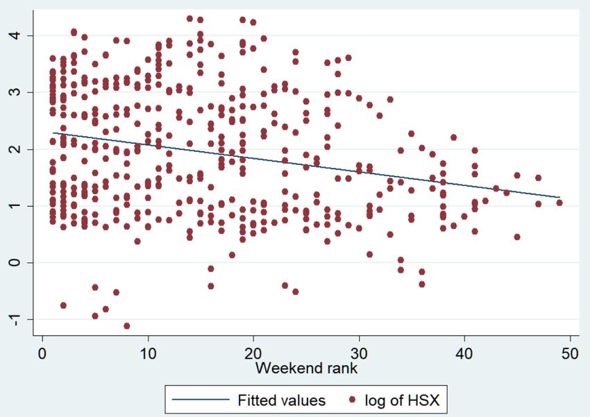
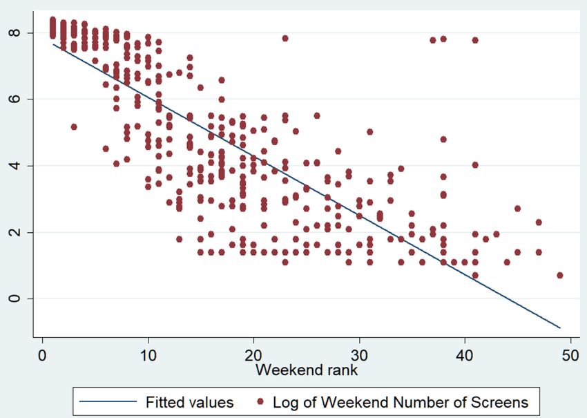
Q-Q Plot HSX Q-Q Plot log of HSX

Figure 15: Q-Q plot of "HSX" Figure 16: Q-Q plot of "log of HSX"

A Q-Q plot helps to graphically verify if a variable is distributed normally. If it is, the distribution

resembles a straight line with a 45° slope. Figure 15 shows that the variable “HSX” is not normally

distributed, but right-skewed. After logging the variable (Figure 16) it resembles a normal distribution.

 4.3. Correlation

 Independent variable – dependent variable

 When I investigate the correlation between the individual variables to examine the relationship,

 I do not see results that are unpredictable. The variables “log of Twitter volume” and “log of

 HSX price” have the highest correlation of 0.7810 (at a significance level of 0.05), which means

 that they have a strong positive relationship. This might be valuable but could also be random,

 as correlation does not say anything about causation. “weekend rank” has a negative correlation

 with all other variables. It is the only variable where a lower number indicates greater success.

 “log of weekend screens” is the only variable that does not correlate with “log of HSX price”

 37

on a 5% significance level (the star in brackets in figure 17 indicates a significance level of

95%), which means it is the first variable I will drop, as it will not offer relevant information.

Figure 17: Correlation table for all variables

The correlation table shows the strength of the linear relationship between all pairs of two

variables in my data set. The darker the green colour the stronger the relationship is

(correlation can take on values between -1 and +1, where -1 is a perfect negative relationship,

0 means no relationship at all and +1 is a perfect positive relationship). When studying the

table, I see that the variables I am especially interested in, “log of Twitter volume” and “log of

Twitter index”, have the highest correlation with the “log of HSX”, followed by “log of

Wikipedia hits” and “log of Google Trends“. Variables that show success at the box office

have the lowest correlation with “log of HSX”.

 38

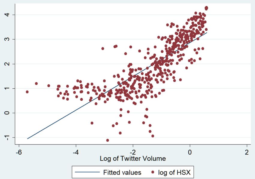
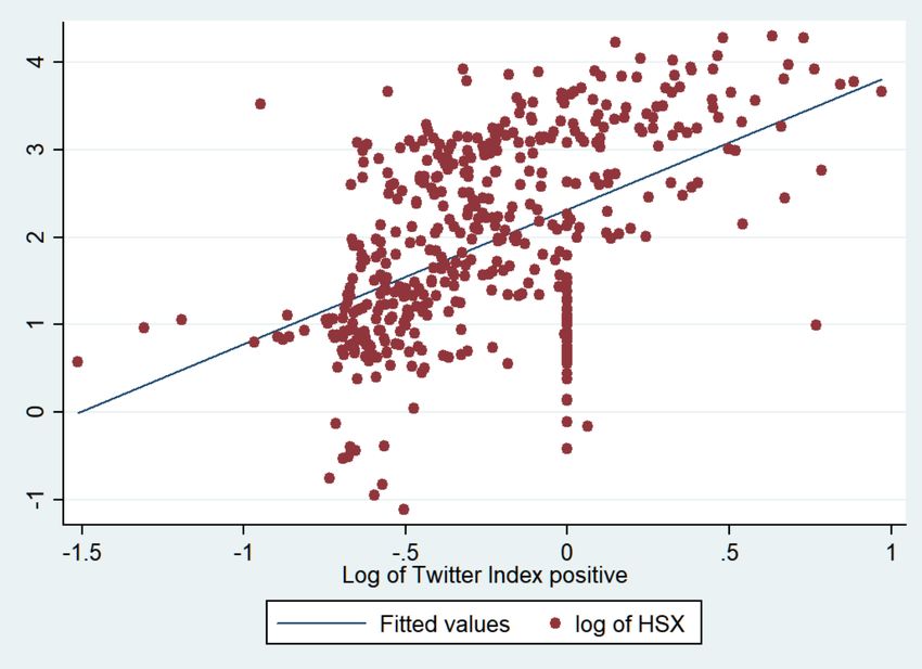
To further examine the relationship between the variables I create a two-way scatterplot with a

line of best fit. The line indicates a strong and positive correlation between the two variables

“log of HSX” and “log of Twitter volume”.

Figure 18: Twoway linear prediction plot between “log of HSX” and “log of Twitter volume”

As indicated in the correlation table, the correlation between “log of HSX” and “log of Twitter

volume” is strong and positive. I include correlation graphs of “log of HSX” and “log of Twitter

index positive”. All other correlation tables are attached in the appendix starting on page 63.

 39