Leveraging Simulation for Computer Vision - CMU's Robotics Institute
←
→
Page content transcription
If your browser does not render page correctly, please read the page content below
Leveraging Simulation for Computer
              Vision
                    Rawal Khirodkar
                           May, 2019
                       CMU-RI-TR-19-11

                 The Robotics Institute
             Carnegie Mellon University
           Pittsburgh, Pennsylvania 15213

                   Thesis Committee:
                    Kris Kitani, Chair
                     Deva Ramanan
                        David Held
                        Lerrel Pinto

      Submitted in partial fulfillment of the requirements
        for the degree of Master of Science in Robotics
            Copyright c 2019 Rawal Khirodkar
Abstract
A large amount of labeled data is required to train deep neural networks. The process of data
annotation on such a large scale is expensive and time-consuming, especially for complex vision
tasks like object pose estimation, semantic segmentation. A promising alternative in this regard,
is to use simulation to generate labeled synthetic data. However, a network trained solely on
synthetic data may not generalize to real data. This is the problem of domain gap, when the training
data distribution differs from the test data distribution.

There are two popular solutions to reducing domain gap, domain adaptation (DA) and domain
randomization (DR). The recently proposed DR has shown promise in control based problems
and warrants a study in computer vision. This thesis aims to provide a scientific study of DR with
a special focus on its applications in computer vision.

The thesis is composed of three parts.

In the first part, we provide an empirical analysis of DR in the context of object detection and pose
estimation. Another key contribution as part of our analysis is a semi-automatic pipeline to build
3D simulators for surveillance scenes.

In the second part, we provide a theoretical analysis of DR. The highlights here include its general-
ization error bound, a comparison with DA and its limitations.

Finally, in the third part, we propose adversarial domain randomization (ADR) as a solution to DR’s
limitations. We evaluate ADR along with DR on image classification, object detection, object pose
estimation on real world datasets. Our evaluations showcase ADR as a more data efficient ap-
proach than DR.

                                                  I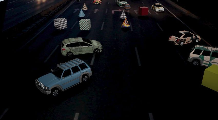
Acknowledgements
   Journeys in life are rarely made alone, and the one that this thesis represent is no different.
   First, I want to thank my advisor Kris Kitani, for providing an atmosphere where I could pursue
any and all of my ideas, and for teaching me to aim high and think big. There were moments when
you were more confident in my abilities than I was - thank you for that. I want to thank Donghyun
for being the mentor figure I needed. I would like to thank Han Zhao along with Aashi Manglik,
both of whom very graciously agreed to go over proofs presented in this thesis. I would like to
thank my labmates, Tanya Marwah, Xiaofang Wang, Shashank Tripathi, Yan Xu for the numerous
brainstorm sessions.
   In addition, I am lucky to have friends who I know will last a lifetime: Akshita Mittel, Nilesh
Kulkarni, Siva Chaitanya, Ishan Nigam, Akshat Agrawal, Sumit Kumar. They are the reason be-
hind my numerous memories at CMU. Finally, at the risk of sounding pretentious, and with the
cognizance that I never fully can, I want to acknowledge the roles played by the three people clos-
est to me: my mother, Kiran Khirodkar (who gifted me my love for books), my father, Sheshrao
Khirodkar (who, amongst other things is responsible for my love for computers), my elder sister,
Sneha Khirodkar (who was always the smarter sibling, but didn’t know it).
   A few words rarely ever capture the true significance of people, but we try.

                                                 II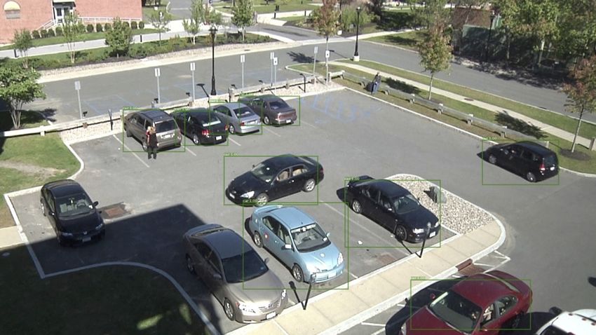
Contents

1   Introduction                                                                                             1
    1.1   Overview . . . . . . . . . . . . . . . . . . . . . . . . . . . . . . . . . . . . . . . . . . .     1
    1.2   Domain Randomization . . . . . . . . . . . . . . . . . . . . . . . . . . . . . . . . . .           1
    1.3   Contributions of this thesis . . . . . . . . . . . . . . . . . . . . . . . . . . . . . . . .       2
    1.4   Related Publications . . . . . . . . . . . . . . . . . . . . . . . . . . . . . . . . . . . .       2

2   Domain Randomization: An Empirical Analysis                                                              3
    2.1   Introduction . . . . . . . . . . . . . . . . . . . . . . . . . . . . . . . . . . . . . . . . .     3
    2.2   Related Work . . . . . . . . . . . . . . . . . . . . . . . . . . . . . . . . . . . . . . . .       4
    2.3   Method . . . . . . . . . . . . . . . . . . . . . . . . . . . . . . . . . . . . . . . . . . . .     5
    2.4   Detection and Pose Estimation Network . . . . . . . . . . . . . . . . . . . . . . . . .            8
    2.5   Experiments . . . . . . . . . . . . . . . . . . . . . . . . . . . . . . . . . . . . . . . . .      8
    2.6   Discussion . . . . . . . . . . . . . . . . . . . . . . . . . . . . . . . . . . . . . . . . . .    13

3   Domain Randomization: A Theoretical Analysis                                                            15
    3.1   Introduction . . . . . . . . . . . . . . . . . . . . . . . . . . . . . . . . . . . . . . . . .    15
    3.2   Preliminaries . . . . . . . . . . . . . . . . . . . . . . . . . . . . . . . . . . . . . . . . .   16
    3.3   Domain Randomization . . . . . . . . . . . . . . . . . . . . . . . . . . . . . . . . . .          17
    3.4   DR as ᾱ-Source Domain . . . . . . . . . . . . . . . . . . . . . . . . . . . . . . . . . .        18
    3.5   Discussion . . . . . . . . . . . . . . . . . . . . . . . . . . . . . . . . . . . . . . . . . .    19

4   Adversarial Domain Randomization                                                                        20
    4.1   Introduction . . . . . . . . . . . . . . . . . . . . . . . . . . . . . . . . . . . . . . . . .    20
    4.2   Method . . . . . . . . . . . . . . . . . . . . . . . . . . . . . . . . . . . . . . . . . . . .    21
    4.3   Experiments . . . . . . . . . . . . . . . . . . . . . . . . . . . . . . . . . . . . . . . . .     23
    4.4   Discussion . . . . . . . . . . . . . . . . . . . . . . . . . . . . . . . . . . . . . . . . . .    30

5   Future Work                                                                                             32

                                                      III
6   Appendix                                                                                            33
    6.1   Derivation of Generalization Error Bound . . . . . . . . . . . . . . . . . . . . . . . .      33
    6.2   CLEVR: Color Classification . . . . . . . . . . . . . . . . . . . . . . . . . . . . . . . .   35
    6.3   Syn2Real: Object Classification . . . . . . . . . . . . . . . . . . . . . . . . . . . . . .   36
    6.4   VIRAT: Depth Estimation . . . . . . . . . . . . . . . . . . . . . . . . . . . . . . . . .     36

                                                    IV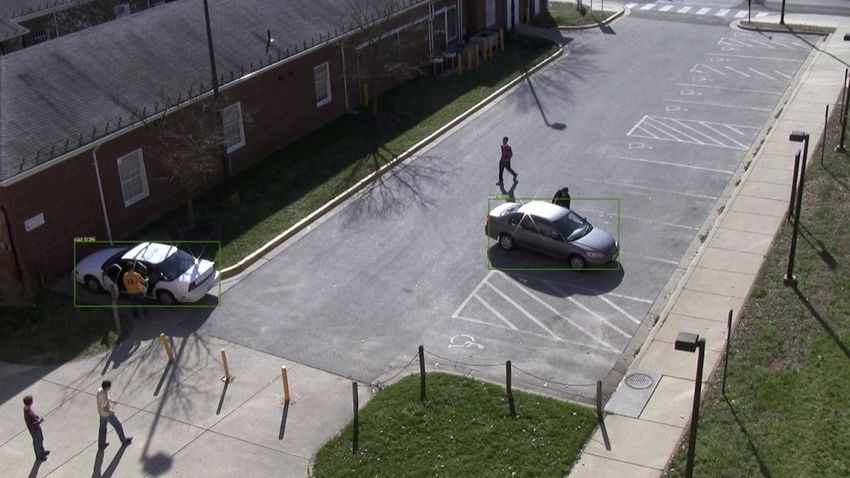
List of Tables

 2.1   Detection results tested on VIRAT, EPFL-Car, UA-DETRAC dataset.          . . . . . . . .   10
 2.2   Pose estimation results tested on EPFL-Car and UA-DETRAC datasets. . . . . . . .           12

 4.1   Effect of data size on DR and ADR, target classification accuracy for Syn2Real . . .       26
 4.2   Effect of unlabeled target data with ADR on Syn2Real . . . . . . . . . . . . . . . . .     27
 4.3   Effect of data size on DR and ADR, Faster-RCNN’s AP at 0.7 IoU on VIRAT. . . . .           27
 4.4   Effect of unlabeled target data with ADR on VIRAT. . . . . . . . . . . . . . . . . . .     28

                                               V
List of Figures

 2.1   3D background modeling from a single image with camera parameter estimation.                         5
 2.2   Labeled synthetic data generated using Unreal Engine. . . . . . . . . . . . . . . . .                6
 2.3   Labeled synthetic data generation using domain randomization. . . . . . . . . . . .                  7
 2.4   Scenes from VIRAT and UA-DETRAC dataset generated using domain randomiza-
       tion. . . . . . . . . . . . . . . . . . . . . . . . . . . . . . . . . . . . . . . . . . . . . . .    7
 2.5   Car detection and pose estimation using modified Faster-RCNN. . . . . . . . . . . .                  8
 2.6   Qualitative analysis of detection on VIRAT 1, VIRAT 2 and UA-DETRAC Night. . .                      11
 2.7   Qualitative analysis of pose estimation on EPFL-Car and UA-DETRAC . . . . . . .                     12
 2.8   An ablation study for detection across VIRAT, EPFL-Car and UA-DETRAC. . . . .                       13
 2.9   An ablation study for pose estimation on EPFL-Car. . . . . . . . . . . . . . . . . . .              14

 3.1   A visualization of the domains using simplex ∆(N = 5). The corners of ∆ are the
       source domains S1 , . . . , S5 and the point T is the target domain. Any interior point
       Sα ∈ ∆ is the upper bound for generalization error T (h∗α ) and the point T is T (h∗T ).
       The distance between Sα and T is d = 2γα + dH∆H (Dα , DT ). The data generated
       using DR is the centre of ∆. . . . . . . . . . . . . . . . . . . . . . . . . . . . . . . . .        18

 4.1   πω is the policy with parameter ω, g is the simulator which takes θ as input and
       generates a labeled data sample x, y. The learner h is trained to minimize `(h(x), y)
       on the data sample. πω is rewarded to maximize the learner’s loss. . . . . . . . . . .              22
 4.2   Image classification (6 classes) for CLEVR. . . . . . . . . . . . . . . . . . . . . . . . .         23
 4.3   Effect of data size on DR, ADR and ADR+DA, target classification accuracy on
       CLEVR averaged over 10 independent runs. . . . . . . . . . . . . . . . . . . . . . . .              24
 4.4   Image classification (12 classes) for Syn2Real. . . . . . . . . . . . . . . . . . . . . . .         25
 4.5   A comparison of source data for VIRAT1 from DR and ADR along with ground
       truth instance segmentation map. . . . . . . . . . . . . . . . . . . . . . . . . . . . . .          28
 4.6   A comparison of source data for VIRAT2 from DR and ADR along with ground
       truth instance segmentation map. . . . . . . . . . . . . . . . . . . . . . . . . . . . . .          29

                                                    VI
4.7   Object spawn probability (πω ) visualized as a heat-map. The warmer colors indicate
      higher probability which correspond to small/truncated/occluded objects in the
      image. . . . . . . . . . . . . . . . . . . . . . . . . . . . . . . . . . . . . . . . . . . . . .   30
4.8   Object detection performance of Faster-RCNN trained on 100k images generated by
      ADR . . . . . . . . . . . . . . . . . . . . . . . . . . . . . . . . . . . . . . . . . . . . .      31

6.1   ADR sample probability over size dimension according to πω averaged over 10 runs.
      small-size are the two smallest sizes and large-size are the two largest sizes. . . . .            36
6.2   ADR πω after generating 100k images on Syn2Real Image Classification task. ADR
      increases the sample generation probability of confusing classes like {bike, mbike}
      and {bus, car, truck, train} whereas easier classes like {knife, plant, aero} see a
      decrease in generation probability. . . . . . . . . . . . . . . . . . . . . . . . . . . . .        37
6.3   Source data for VIRAT scenes generated using ADR with the ground truth depth
      map. . . . . . . . . . . . . . . . . . . . . . . . . . . . . . . . . . . . . . . . . . . . . .     38
6.4   Depth estimation output from an FCN trained on data generated by ADR for VIRAT 39

                                                  VII
Chapter 1

Introduction

1.1    Overview
Simulation plays an important role in fields like robotics [56], physics [3], biology [8]. We believe,
it seems to be a promising solution to an important problem in computer vision, data annotation.
Many state-of-the-art systems in computer vision are based on deep neural networks. These sys-
tems are notoriously known to require large scale training data often of the order of millions of
samples. A natural question therefore arises, how much data is enough? [25] did an important
study which shows that the performance of these state-of-the-art systems does not plateau even
after training on billions of samples. A manual annotation process on such a scale can be expen-
sive and time-consuming, especially for complex vision tasks like semantic segmentation where
labels are difficult to specify. It is, thus, natural to explore simulation for generating synthetic data
as a cheaper and quicker alternative to manual annotation.
   However, while use of simulation makes data annotation easier, it results in the problem of
domain gap. This problem arises when the training data distribution - source domain differs from
the test data distribution - target domain. In this case, learners trained on synthetic data would
suffer from high generalization error. There are two popular solutions to reducing domain gap,
(1) the well studied paradigm of domain adaptation (DA) [50] and (2) the recently proposed do-
main randomization (DR) [47]. DR has shown promise in control based problems and warrants a
study in computer vision. This thesis aims to provide a scientific study of DR as a tool to leverage
simulation for computer vision.

1.2    Domain Randomization
Given a vision task, we can always find critical features in data most useful for the task. For ex-
ample, shape of the car is more useful for car detection than the color of the car. The underlying

                                                   1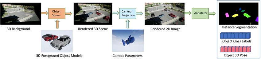
assumption when using simulation for training is that we approximate these critical features from
real data as closely as possible in synthetic data. Under this assumption, these features are also
called as domain invariant features, features which are common to real data (target domain) and
synthetic data (source domain).
   The central idea of DR is to generate synthetic data by randomizing over features which are not
critical or domain-invariant. Therefore, a model trained on such varied synthetic data generalizes
to real-world without any further fine-tuning. The central idea of DR is to generate synthetic data
by randomizing over features which are not critical or domain-invariant.

1.3       Contributions of this thesis
In this thesis, we take steps towards understanding the advantages and limitations of DR both
empirically and theoretically. Specifically:

   1. In Chapter 2, we empirically analyse DR in the context of object detection and pose esti-
         mation in surveillance setting. We propose a semi-automatic pipeline based on Unreal En-
         gine [37] to model surveillance scenes in 3D capable of performing DR. Our analysis includes
         an ablative study which examines the effect of different randomizations like appearance ran-
         domization, size randomization, shape randomization, light augmentation and distractors.

   2. In Chapter 3, we theoretically analyse DR. Specifically, 1) we provide a bound for its gen-
         eralization error, 2) we show that randomization results in a lower error bound than not
         randomizing at all, 3) we highlight key limitations of DR.

   3. In Chapter 4, as a solution to DR’s limitations, we develop Adversarial Domain Randomiza-
         tion (ADR), a more data efficient variant of DR.

1.4       Related Publications
Most ideas described in this thesis have appeared (or are under review) in the following publica-
tions:

   • R. Khirodkar, D. Yoo and K. Kitani. Domain Randomization for Scene-Specific Car Detection
         and Pose Estimation. IEEE Winter Conference on Applications of Computer Vision (WACV),
         2019.

   • (under review) R. Khirodkar, D. Yoo and K. Kitani. Adversarial Domain Randomization.
         IEEE International Conference on Computer Vision (ICCV), 2019.

                                                   2
Chapter 2
Domain Randomization: An
Empirical Analysis
2.1 Introduction
For our analysis, we choose the problem of car detection and pose estimation in surveillance
videos. The setup is as follows, consider the scenario in which a surveillance system is installed
in a novel location and an image-based car detection and pose estimation model must be trained.
A common approach is to frame this as a supervised learning problem and re-use models pre-
trained on large visual datasets such as COCO [21], KITTI [10], PASCAL3D+ [53]. However, the
data distribution of these off-the-shelf datasets can vary significantly from the in-focus surveil-
lance setting. For instance, the camera elevations of a close circuit camera are different from a
vehicle mounted camera, a representative case of the KITTI dataset. Fine-tuning a pre-trained
model using a small scene-specific dataset is often performed to ensure good performance dur-
ing inference. We would like to highlight two major shortcomings of this approach, (1) obtaining
a new dataset for each new surveillance location is not scalable due to expensive human hours
spent in gathering these annotations, (2) another problem is overfitting to this small domain spe-
cific dataset during training. We provide an alternative solution to address these shortcomings
using a synthetic data generation pipeline which is scalable and robust to data variance.
Our goal is to develop a method for training a scene-specific car pose estimation and detection
model without real annotations. This is an ill posed zero-instance learning problem, however, we
do have access to three important priors here: (1) 3D scene geometry, (2) camera parameters and
finally (3) priors on the geometry and appearance of the object of interest (such as cars) available in
the form rich3D CAD models. We model this domain specific knowledge in the form of a synthetic
data generation pipeline to compensate for the absence of real training data. In this pipeline, we
3model the scene in 3D using state-of-the-art rendering engine Unreal Engine 4. An upside of using
synthetic data is that we are capable of generating pixel-level accurate annotations like instance
segmentation, depth map, category labels, 3D object locations and pose annotations. However, an
underlying challenge here is that using synthetic data as the sole source of supervision can result
into poor performance during inference on real data.
This is the aforementioned problem of ’domain gap’ [5,31,33,50]. The model trained on synthetic
data can over-fit to it, not generalizing well to real data. We use domain randomization (DR) as a
solution to bridge the domain gap. A key advantage of DR is that it provides a solution for domain
gap in the data generation phase rather than the algorithm phase. This allows us to modularize our
solution nicely into two modules, data generation and learning model. Only the data generation
module addresses domain gap, which provides us flexibility of making different design choices
for our learning model. We provide an end-to-end framework capable of supporting multiple
learning models which is an important attribute of a scalable system.
The contributions of this analysis are: (1) synthetic data generation pipeline, we encode known
information like 3D scene geometry, camera parameters, object shape and appearance into rich an-
notated data, (2) a supportive ablation study for DR, we use DR to generate diverse synthetic data
to span the space of realistic images. We conduct an ablation study to examine the effect of individ-
ual randomization components like texture randomization, light augmentation and distractors, (3)
evaluations on diverse datasets, we benchmark our approach on VIRAT [29], UA-DETRAC [24],
EPFL Cars Datasets [30] for the task of car detection and pose estimation.
2.2 Related Work
Our analysis is related to object detection and pose estimation, synthetic data for computer vision,
domain adaptation and domain randomization.
3D Models for Object Detection and Pose Estimation Car detection and pose estimation is a
well studied problem in the literature(see e.g., [28], [27], [40]). The classical problem of 6 DoF
pose estimation of an object instance from a single 2D image has been considered previously as a
purely geometric problem known as the perspective n-point problem (PnP). Several closed form and
iterative solutions assuming correspondences between 2D keypoints in the image and a 3D model
of the object can be found in [18].
Synthetic Data for Computer Vision Dhome et al. used synthetic models to recognize objects
from a single image [26]. For pedestrian detection, computer generated pedestrian images were
used to train classifiers [11]. 3D simulation has been used for multi-view car detection [4] [54] [13].
Sun and Saenko [44] trained 2D object detector with synthetic data generated by 3D simulation.
Domain Adaptation Ganin and Lempitsky proposed a domain adaptation method where the
4Figure 2.1: 3D background modeling from a single image with camera parameter estimation.
learned feature are invariant to the domain shift [55]. [52] suggested a multichannel autoencoder
to reduce the domain gap between real and synthetic data. SimGAN [42] used domain adaption
for training eye gaze estimation systems on synthetic eye images. They solved the domain shift
problem of synthetic images using a GAN based refiner that converts the synthetic images to the
refined images. The refined images have similar noise distribution to real eye images.
Domain Randomization [39] used DR to fly a quadrotor through indoor environments. [7] trained
an agent to play Doom and generalize to unseen game levels. [47], [14], [36], [35] used DR for
grasping objects. Tremblay et al. performed car detection with DR [48]. [45] proposed object
orientation estimation for industrial part shapes that is solely trained on synthetic views rendered
from a 3D model. They used DR to reduce the gap between synthetic data and real data.
2.3 Method
Our goal is to detect all the cars and estimate their orientations in a specific scene. We assume
that scene geometry and camera parameters are given, and use that information along with a rich
library of 3D CAD models to generate annotated synthetic data. As alluded to earlier, the main
challenge which must be addressed is how to ensure generalization of our network trained on
synthetic data to unseen real data. To address this challenge, we employ DR in the data generation
step to create synthetic data with enough variations such that the trained network does not over-fit
to the synthetic data distribution, thus generalizing to real data during inference.
In this section, we first describe our scene-specific data generation methodology followed by
details about DR.
5Figure 2.2: Labeled synthetic data generated using Unreal Engine.
2.3.1 Synthetic Data Generation
We use the state-of-the-art rendering platform Unreal Engine 4 for data generation. The first step
is to encode the known scene geometry and camera parameters in our model with minimal user
supervision. Figure 2.1 shows a schematic overview of this step. Here, we assume access to one
image of the scene from the surveillance camera. First foreground objects are removed from this
image using in-painting (or background extraction from video) giving us the scene’s background
image. A textureless 3D layout is constructed from the known scene geometry. The layout is then
textured using homographic projections of scene’s background image into different views giving
us an approximate box-shaped 3D model of the background. The extrinsic camera parameters
are estimated using 2D to 3D point correspondences provided by the user, we also perform grid
search over an initial estimate of camera intrinsics if the knowledge of these exact parameters are
not known. The scale transformation of an unit measure in the real scene to the synthetic scene is
provided by the user. Finally, these assets, namely the camera and 3D textured layout represent
the known camera parameters and scene geometry respectively.
We now proceed to encode rich priors about the foreground objects appearing in the scene
using a large collection of 3D CAD models (see Figure 2.2). 3D models in standard mesh repre-
sentations are very high dimensional but interpretable and finite dimensional. By virtue of design,
this gives us excellent control over the object’s characteristic properties like scale, shape, texture.
We now proceed to render foreground objects with desirable properties in the 3D layout. This
flexibility is critical for our DR setup. After the completion of rendering, we use Unreal Engine’s
ray tracing to generate pixel level accurate ground truth labels like instance segmentation, class
labels and pose annotations.
2.3.2 Domain Randomization
The key idea here is to generate enough variations in the image space to avoid model overfitting.
Also, the variations using DR make the model robust to object appearances and light condition.
6Figure 2.3: Labeled synthetic data generation using domain randomization.
Figure 2.4: Scenes from VIRAT and UA-DETRAC dataset generated using domain randomization.
Concretely, we introduce randomization by varying the following aspects of the scene.
• Content Variation: A random number of objects are placed randomly in the 3D background
with varying orientation. To achieve shape and size variations we use an array of 5 different
types of car models, the model’s dimensions are randomly perturbed to provide more fine
geometric variations. We also place 3D distractor objects in the scene like pedestrians, cones,
spheres at varying dimensions to model the appearance of uninteresting objects in the scene.
• Style Variation: The style variation is achieved by randomly varying the color, texture of all
the objects. We use a texture bank of 50 textures for this purpose. Furthermore, we apply
light augmentations to capture the varying shadow conditions and time of day changes, we
also varying the lightning conditions by changing the number of sources along with the
location, orientation and luminosity. The generated image also undergoes random changes
in contrast and brightness to model slight appearance changes of the background.
72.4 Detection and Pose Estimation Network
For the learning model, our method adopts the Faster-RCNN [38]/Network-on-Convolution meta-
architecture. The network consists of a shared backbone feature extractor for the full-image, fol-
lowed by region-wise sub-networks (heads) that predict the car’s yaw angle with respect to the
camera coordinate system in addition to traditional 2D bounding box and class label.
Our initial experiments indicated framing the problem of pose estimation as a classification
task more favorably than as a regression task. Classification over-parametrizes the problem, and
thus allows the network more flexibility to learn the task. As, the pose angles are bounded by
[−π, π], we quantize this space into 36 bins.
For our backbone network, we use the Feature Pyramid Network setup with ResNet101 archi-
tecture. Figure 2.5 illustrates our model. We define a multi-task loss function (L) for sampled
region proposal as follows:
L = Lclass + Lbbox + Lpose
where Lclass is the object classification loss, Lbbox is the bounding box regression loss as defined
in [38]. Lpose is the pose label classification loss.
Figure 2.5: Car detection and pose estimation using modified Faster-RCNN.
2.5 Experiments
We analyse DR on three datasets VIRAT, EPFL-Car and UA-DETRAC for the tasks of car detection
and pose estimation.
8• VIRAT dataset is designed to be realistic, natural and challenging for video surveillance
domains in terms of its background clutter, diversity in scenes. The captured video are
recorded at 25 frames per seconds (fps) at the resolution of 1920 × 1080 pixels.
• EPFL-Car dataset contains 20 sequences of cars as they rotate by 360 degrees. The dataset
contains images with variation in background, and slight changes in camera elevation recorded
at 376 × 250 pixels.
• UA-DETRAC is a challenging real-world multi-object detection benchmark consisting of 10
hours of videos captured at 24 different locations. The videos are recorded at 25 frames per
seconds (fps), with resolution of 960 × 540 pixels.
We perform evaluations on two scenes from VIRAT dataset, entire EPFL-Car dataset and two
scenes from UA-DETRAC dataset. 10,000 synthetic images are rendered for each scene at the
resolution of 1440×810 pixels for each variation in the ablation study with 80:20 split as the training
and validation set. Furthermore, 8000 images per scene (VIRAT), 2300 images (EPFL-Car), 2000
images per scene (UA-DETRAC) constitutes our real data for evaluations. A random 70:20:10 split
of the real images per scene makes up our training, validation and test set respectively.
Note that to capture the background and camera elevation changes in the EPFL-Car dataset, we
also randomly perturb the camera parameters and background textures during data generation.
For all our experiments, we compare six models.
• SS-scratch, initialized with random weights and trained on scene specific synthetic data
without DR.
• SS-finetune, initialized with COCO and fine-tuned on scene specific synthetic data without
DR.
• SS+DR-scratch, initialized with random weights and trained on scene specific domain ran-
domized data.
• SS+DR-finetune, initialized with COCO and fine-tuned on scene specific domain random-
ized data.
• Real-0.5, initialized with COCO and fine-tuned on 50% real training data.
• Real, initialized with COCO and fine-tuned on the entire real training data.
Without DR: We use 4 car models with fixed dimensions, 7 colors, constant lighting conditions
without contrast or brightness augmentation. We do not use cubes, spheres or cones as distractors,
however pedestrians are still rendered.
To ensure consistency, we use similar model architecture as reported in section 2.4, same hyper-
parameters and training regime. We also compare our models against the baseline of an off-the-
shelf pre-trained network for the car detection and pose estimation.
9VIRAT 1 VIRAT 2 EPFL-Car UA-DETRAC Night UA-DETRAC Street
Model
AP@0.5 AP@0.75 AP@0.5 AP@0.75 AP@0.5 AP@0.75 AP@0.5 AP@0.75 AP@0.5 AP@0.75
COCO 92.9 75.6 85.5 43.0 55.7 28.5 62.9 34.5 78.3 51.8
SS-scratch 54.2 37.8 49.1 18.9 31.5 0.4 51.0 20.4 36.7 12.8
SS-finetune 80.3 39.5 54.6 19.2 38.1 3.5 52.5 21.9 38.3 15.0
SS+DR-scratch 98.8 56.4 81.7 34.3 48.6 7.4 78.7 40.6 52.1 29.6
SS+DR-finetune 98.9 62.6 97.6 48.8 76.8 22.9 82.8 56.7 87.3 51.2
Real-0.5 94.3 82.1 87.5 57.4 62.3 48.1 82.3 67.1 84.0 44.2
Real 98.9 84.8 98.1 61.8 82.7 60.8 90.1 73.3 92.0 65.1
Table 2.1: Detection results tested on VIRAT, EPFL-Car, UA-DETRAC dataset.
2.5.1 Object Detection
The pre-trained model we use in detection evaluations is a car detector trained on 5010 car images
from the COCO dataset (referred as COCO henceforth). We report average precision for bounding
box regression at IoU={0.5, 0.75}.
Quantitative Analysis: Table 2.1 shows the detection results tested on VIRAT, EPFL-Car, and UA-
DETRAC dataset. Our SS+DR-finetune achieves the best performance in the most cases and out-
performs Real-0.5. We hypothesize this is due to overfitting on limited real data which is avoided
by design in DR. Furthermore, our model trained only on synthetic data is competitive to the
model trained on the entire real data at IoU=0.5.
SS+DR-finetune outperforms the off-shelf baseline COCO by more than 6% and this margin
only increases when the scene distribution differs considerably from the off-shelf dataset’s distri-
bution.
Qualitative Analysis: Figure 2.6 shows qualitative detection results, in this section we compare
COCO, SS-finetune, and SS+DR-finetune. COCO fails in cases of severe object occlusion (first
row), unusual shadows (first row, second row) and object truncation (second row, third row). Even
though we explicitly model object occlusions and truncation in our synthetic data, SS-finetune fails
to generalize to real data. This is because the deep network latches on to the synthetic dataset’s
biases, our SS+DR-finetune does not suffer from any of these shortcomings.
Furthermore, we found that the bounding boxes of SS+DR-finetune are more accurate than
SS-finetune. We argue that this is because SS-finetune overfits to the height-to-width distribution
of bounding boxes in the synthetic dataset. DR helps mitigates this problem by randomizing the
dimensions and shapes of the 3D models during data generation, thus directly providing enough
variance in the bounding box distribution. This regularizes SS+DR-finetune.
10COCO SS-finetune SS+DR-finetune
Figure 2.6: Qualitative analysis of detection on VIRAT 1, VIRAT 2 and UA-DETRAC Night.
2.5.2 Pose Estimation
Similar to COCO for detections, we benchmark our models against Deep3DBox [27] trained on
KITTI dataset for 3D bounding box estimation. To ensure consistency, we use ground truth detec-
tions as our region proposals for all our experiments and extract features using this proposals for
the task of pose estimation.
Quantitative Analysis: Table 2.2 shows the pose estimation results, we benchmark our results
on EPFL-Car and UA-DETRAC datasets. EPFL-Car already has car pose annotations, we manu-
ally annotate two scenes from UA-DETRAC with pose annotations. We report pose classification
accuracy Acc10o ↑ at 10o degree quantization and median error angle MedErr↓.
Our SS+DR-finetune achieves the best results that are competitive to Real-0.5 and Real in all
the cases even though we don’t use any real images for training.
Qualitative Analysis: Figure 2.7 shows qualitative pose results, in this section we compare Deep3DBox-
KITTI, SS-finetune, and SS+DR-finetune on images from EPFL-Car and UA-DETRAC Street scene.
Note we assume ground truth bounding boxes as input for this analysis.
The camera perspective is significantly different for KITTI and EPFL-Car dataset, this results
in poor performance of Deep3DBox on EPFL-Car images. However, SS-finetune performs better
11EPFL-Car UA-DETRAC Night UA-DETRAC Street
Model
Acc10o ↑ MedErr↓ Acc10o ↑ MedErr↓ Acc10o ↑ MedErr↓
o o
Deep3DBox-KITTI 0.67 18.3 0.41 28.0 0.58 17.7o
o o
SS-scratch 0.35 46.2 0.18 63.1 0.45 38.3o
SS-finetune 0.66 16.1o 0.51 31.8o 0.72 23.0o
o o
SS+DR-scratch 0.72 10 0.74 21.6 0.61 10.4o
o o
SS+DR-finetune 0.86 6.6 0.83 14.2 0.87 13.2o
o o
Real-0.5 0.91 5.4 0.93 11 0.96 5.8o
Real 0.96 6.1o 0.97 10.4o 0.97 3.4o
Table 2.2: Pose estimation results tested on EPFL-Car and UA-DETRAC datasets.
Real Image Deep3DBox-KITTI SS-finetune SS+DR-finetune
θ = 308.76o θ = 280.3o θ = 315.0o θ = 305.0o
Mean Angle Error = θ̄error θ̄error = 73.8o θ̄error = 21.4o θ̄error = 9.5o
Figure 2.7: Qualitative analysis of pose estimation on EPFL-Car and UA-DETRAC
than Deep3DBox in our analysis, as we assume ground truth bounding box proposals, this is due
to the task specific network learning appearance invariant features for pose prediction.
On the UA-DETRAC dataset, the camera perspective is much more similar to KITTI dataset,
however the car appearance is significantly different from KITTI. Notice the top right yellow car
was flipped by Deep3DBox as it could not distinguish between the head and the tail. Our model
SS+DR-finetune performs consistently well across these evaluations.
2.5.3 Ablation Study
We conduct ablation studies to examine the effects of textures (T), light augmentation (LA), ge-
ometrical variations to object shapes (G), addition of distractors (D), and full randomization(T +
LA + D + G).
We compare (1) LA + G + D, no textures, the object models are rendered without texture vari-
12Figure 2.8: An ablation study for detection across VIRAT, EPFL-Car and UA-DETRAC.
ations with a fixed color scheme, (2) T + G + D, no light augmentations, the lighting conditions
are held constant, no contrast or brightness changes introduced, (3) T + LA + D: no geometrical
variations, every object has fixed dimension, (4) T + LA + G: no distractors, (5) T + LA + D + G,
full randomization.
Figure 2.8 shows the comparison chart of the bounding boxes results at IoU=0.5 for the afore-
mentioned randomization conditions for 3 datasets. Removing textures (LA + G + D) results in
the most performance drop followed by removing geometrical variations for the task of object
detection. Thus, we conclude that varying object appearance and shape and size are two critical
components for object detection.
Figure 2.9 shows the comparison chart of the pose estimation results on EPFL-Cars dataset.
We assume ground truth bounding box proposals. Removing geometric variations results in the
most performance drop followed by the object appearance. The pose estimation head is learning
appearance invariant features and is more sensitive to geometry of the object.
2.6 Discussion
To conclude, scene specific treatment along with DR is promising solution for annotation less
setups in surveillance. In this empirical analysis, we proposed a framework to generate rich syn-
thetic annotations which incorporate prior knowledge about the scene. Furthermore, using DR we
13Figure 2.9: An ablation study for pose estimation on EPFL-Car.
ensure any learning algorithm trained on such kind of data would generalize to real data during
inference. We performed studies to analyse the effect of each individual randomization compo-
nents. Compelling results are demonstrated on VIRAT, EPFL-Car and UA-DETRAC datasets for
the detection and pose estimation.
14Chapter 3
Domain Randomization: A
Theoretical Analysis
3.1 Introduction
We ask following key questions: how does DR compensate for the lack of information on target
domain? The answer lies in the design of the simulator used by DR for randomization. The simu-
lator is encoded with target domain knowledge (priors on shape of objects) beforehand. This acts
as a sanity check between the labels of source domain and target domain (cars should not be la-
beled as trucks). Another key design decision involves which simulation parameters are supposed
to be randomized. This plays an important role in deciding the domain invariant features which
help the learner in generalizing to the target domain. Clearly, these domain invariant features are
task dependent, as they contain critical information to solve the task. in car detection, the shape
of a car is a critical feature and has to be preserved in source domain, it is therefore acceptable
to randomize the car’s appearance by adding textures in DR. However, when the task changes
from car detection to a red car detection, car’s appearance becomes a critical feature and can no
longer be randomized in DR. We believe it is important to understand such characteristics of the
DR algorithm. Therefore, as a step in this direction, in section ??, we provide theoretical analysis
of DR. Concretely our analysis answers the following questions about DR: 1) how does it make
the learner focus on domain invariant features? 2) what is its generalization error bound? 3) in
presence of unlabeled target data, can we use it with DA? 4) what are its limitations?
We analyze DR using generalization error bounds from multiple source domain adaptation [1].
The key insight is to view DR as a learning problem from multiple source domains where each
source domain represents a particular subset of the data space. For example, consider the space of
all car images. The images containing a car of a particular make form a subset of that space which
15we refer to as a single source domain. If one were to generate random images across different car
makes, as we do in DR, this can be interpreted as combining data from multiple source domains.
In this section, we first introduce the preliminaries in 3.2 followed by a formal definition of DR
algorithm in 3.3. Lastly, we draw parallels between DR and multiple source domain adaptation
in 3.4 where we also show that the generalization error bound for DR is better than the bound for
data generation without randomization.
3.2 Preliminaries
The notation introduced below is based on the theoretical model for DA using multiple sources
for binary classification [1]. The analysis here is limited to binary classification for simplicity but
can be extended to other tasks as long as the triangle inequality holds [2].
A domain is defined as a tuple hD, f i where: (1) D is a distribution over input space X and
(2) f : X 7→ Y is a labeling function, Y being the output space which is [0, 1] for binary clas-
sification. N source domains are denoted as {hDi , fi i}|N
i=1 and the target domain is denoted
as hDT , fT i. A hypothesis is a binary classification function h : X 7→ {0, 1}. The error (some-
times called risk) of a hypothesis h w.r.t a labeling function f under distribution D is defined
as (h, f, D) := Ex∼D |h(x) − f (x)| . We denote the error of hypothesis h on target domain as
T (h) = (h, fT , DT ) and on ith source domain as i (h) = (h, fi , Di ). As common notation in
computational learning theory, we use T (h) and ˆT (h) to denote the true error and empirical
error on the target domain. Similarly, i (h) and ˆi (h) are defined for ith source domain.
Multiple Source Domain Problem. Our goal is to learn a hypothesis h from hypothesis class
H which minimizes T (h) on the target domain hDT , fT i by only using labeled samples from N
source domains {hDi , fi i}|N
i=1 .
α-Source Domain. We combine N source domains into a single source domain denoted as α-
source domain where α helps us control the contribution of each source domain during training.
PN
We denote by ∆ the simplex of RN , ∆ = {α : αi ≥ 0 ∧ i=1 αi = 1}. Any α ∈ ∆ forms
an α-source domain. The error of a hypothesis h on this source domain (α-error) is denoted as
PN PN
α (h) = i=1 αi i (h). The α input distribution is denoted as Dα = i=1 αi Di .
The multiple source domain problem can now be reduced to training on labeled samples from
α-source domain for various values of α ∈ ∆. We use Dα to sample inputs from X , which are
then labeled using all the labeling functions {hfi i}|N
i=1 . We learn a hypothesis h to minimize the
PN
empirical α-error, ˆα (h) = i=1 αi ˆi (h).
Generalization Error Bound. Let ĥα = argminh ˆα (h) and h∗α = argminh α (h) ĥα and h∗α mini-
mize the empirical and true α-error respectively. We are interested in bounding the generalization
error T (ĥα ) for empirically optimal hypothesis ĥα . However, using Hoeffding’s inequality [41],
16it can be shown that minimum empirical error ˆα (ĥα ) converges uniformly to the minimum true
error α (h∗α ) without loss of generality ĥα converges to h∗α given large number of samples. To
simplify our analysis we instead bound generalization error T (h∗α ) for true optimal hypothesis
h∗α (the bound for ĥα is provided in appendix).
Following the proof for Th. 5 (A bound using combined divergence) in [1], we provide a bound
for generalization error T (h∗α ) below.
Theorem 1. (Based on Th.5 [1]) Consider the optimal hypothesis on target domain h∗T = argminh T (h)
and on α-source domain h∗α = argminh α (h). If γα = minh {T (h) + α (h)}, then
T (h∗α ) ≤ T (h∗T ) + 2γα + dH∆H (Dα , DT )
Remarks: Proof in appendix. T (h∗T ) is the minimum true error possible for the target domain
(clearly, T (h∗T ) ≤ T (h∗α )). γα represents the minimum error using both the target domain and
α-source domain jointly. Intuitively, it represents the agreement between all the labeling functions
involved (target domain and all source domains) γα would be large, if these labeling functions la-
bel an input differently. Lastly, dH∆H (Dα , DT ) is the H∆H divergence between input distributions
Dα and DT . In summary, generalization on target domain T (h∗α ) depends on: (1) difficulty of task
on target domain T (h∗T ); (2) labeling consistency between target domain and source domains γα ;
(3) similarity of input distribution between target and source domains dH∆H (Dα , DT ).
3.3 Domain Randomization
DR addresses the multiple source domain problem by modeling various source domains using
a simulator with randomization. The simulator is a generative module which produces labeled
data (x, y). In practice, DR uses an accurate simulator which internally encodes the knowledge
about the target domain as a target labeling function fT (x), such that y = fT (x). Concretely, let
Θ be the rendering parameter space and DΘ be a probability distribution over Θ. We denote the
simulator as a function g : Θ 7→ X × Y such that g(θ) = {x, y} where θ ∼ DΘ . Simply put,
a simulator g takes a set of parameters θ and generates an image x and its label y. In general,
the DR algorithm generates data by randomly (uniformly) sampling θ from Θ DΘ is set to UΘ , an
uniform distribution over Θ (refer Alg. 1). The algorithm outputs a hypothesis ĥ which empirically
minimizes the loss `(ĥ(xi ), yi ) over M data samples. Note, in our analysis, we set `(ĥ(x), y) to be
|ĥ(x) − y|. learner-update is the parameter update of ĥ using loss `(ĥ(xi ), yi ).
The objective function optimized by these steps can be written as follows:
h i
min E ` h g(θ)x , g(θ)y (1)
h∈H θ∼UΘ
17Algorithm 1 Domain Randomization
Input: g, M
Output: ĥ
1: for i ∈ {1, 2, . . . , M } do
2: θ ∼ UΘ
3: {x, y} = g(θ)
4: ĥ = learner-update(ĥ, x, y)
S1
T
d
S5 Sα S2
S4 S3
Figure 3.1: A visualization of the domains using simplex ∆(N = 5). The corners of ∆ are the
source domains S1 , . . . , S5 and the point T is the target domain. Any interior point Sα ∈ ∆ is the
upper bound for generalization error T (h∗α ) and the point T is T (h∗T ). The distance between Sα
and T is d = 2γα + dH∆H (Dα , DT ). The data generated using DR is the centre of ∆.
3.4 DR as ᾱ-Source Domain
We interpret data generated using DR as labeled data from an α-source domain, specifically α =
[ N1 , . . . , N1 ] (referred as ᾱ hereafter). This captures equal contribution by each sample during train-
ing according to Alg 1. Using Th. 1, we can bound the generalization error for ᾱ-source domain
PN
(DR) by T (h∗T ) + 2γ̄ + dH∆H (Dᾱ , DT ) where γ̄ = minh {T (h) + N1 i=1 i (h)}.
We now compare DR with data generation without randomization or variations. The later is
same as choosing only one source domain for training, denoted as αi -source domain where αi is a
one-hot N -vector indicating domain i ∈ {1, . . . , N }. The generalization error bound for αi -source
domain would be T (h∗T ) + 2γi + dH∆H (Di , DT ) where γi = minh {T (h) + i (h)}.
Refer to Fig. 3.1 for a visualization of generalization error of Sα as a distance measure from
18target domain, we define d = 2γα + dH∆H (Dα , DT ) as the upper bound for |T (h∗α ) − T (h∗T )|.
We wish to find an optimal α which minimizes this distance measure the point in ∆ closest to the
target domain (α2 in Fig. 3.1). However, when no unlabeled target data is available it is best to
choose the centre of ∆ (α = ᾱ) as our source domain. We prove this in lemma 5, which states
that the distance of target domain from the centre of ∆ is less than the average distance from the
corners of ∆.
Lemma 2. For i ∈ {1, . . . , N }, let αi = [0, .. 1 ..0], γi = minh {T (h) + i (h)} and ᾱ = [ N1 , N1 ..., N1 ],
ith
PN
γ̄ = minh {T (h) + N1 i=1 i (h)}, then
N
1 X
2γi + dH∆H (Di , DT ) ≥ 2γ̄ + dH∆H (Dᾱ , DT )
N i=1
Remarks: Proof provided in appendix follows from the convexity of distance measure 2γi +
dH∆H (Di , DT ) with application of Jensen’s inequality [19]. Using this lemma, the corollary 2.1
states that in the absence of unlabeled target data, in expectation DR (centre of ∆) is superior to
data generation without randomization (any other point in ∆).
Corollary 2.1. The generalization error bound for ᾱ-source domain (DR) is smaller than the expected
generalization error bound of a single source domain (expectation over a uniform choice of source domain).
3.5 Discussion
DR is a powerful method that bridges the gap between real and synthetic data. There is a need to
analyze such an important technique, our work is the first step in this direction. We theoretically
show that DR is superior to synthetic data generation without randomization. We also identify
DR’s requirement of a lot of data for generalization.
19Chapter 4
Adversarial Domain Randomization
4.1 Introduction
In our previous analysis, we identify a key limitation: DR requires a lot of data to be effective. This
limitation mainly arises from DR’s simple strategy of using a uniform distribution for simulation
parameter randomization. As a result, DR often generates samples which the learner has already
seen and is good at. This wastes valuable computational resources during data generation. We can
view this as an exploration problem in the space of simulation parameters. A uniform sampling
strategy in this space clearly does not guarantee sufficient exploration in image space. We address
this limitation in here by proposing Adversarial Domain Randomization (ADR), a data efficient
variant of DR. ADR generates adversarial samples with respect to the learner during training. We
implement ADR as a policy whose action space is the quantized simulation parameter space. At
each iteration, the policy is updated using policy gradients to maximize learner’s loss on generated
data whereas the learner is updated to minimize this loss. As a result, we observe ADR frequently
generates samples like truncated and occluded objects for object detection and confusing classes
for image classification.
Finally, we go back to the question posed previously, can we use DR with DA when unlabeled
target data is available? Our reinforcement learning framework for ADR easily extends to incorpo-
rate DA’s feature discrepancy minimization in form of reward for the policy. We thus incentivize
the policy to generate data which is consistent with target data. As a result, we no longer need to
manually encode domain knowledge in the design of the simulator. In summary, the contributions
of our work are as follows:
• Adversarial Domain Randomization: As a solution to DR’s limitations, we propose a more
data efficient variant of DR, namely ADR.
20• Evaluations on Real Datasets for Diverse Tasks: We benchmark our approach on image clas-
sification and object detection on real-world datasets like Syn2Real [34], VIRAT [29].
4.2 Method
We modify DR’s objective (eq.1) by making a pessimistic (adversarial) assumption about DΘ in-
stead of assuming it to be stationary and uniform. By making this adversarial assumption, we
force the learned hypothesis to be robust to adversarial variations occurring in the target domain.
This type of worst case modeling is especially desirable when annotated target data is not available
for rare scenarios.
The resulting min-max objective function is as follows:
h i
min max E ` h g(θ)x , g(θ)y (2)
h∈H DΘ θ∼DΘ
4.2.1 ADR via Policy Gradient Optimization
This adversarial objective function is a zero-sum two player game between simulator (g) and
learner (h). The simulator selects a distribution DΘ for data generation and the learner chooses
h ∈ H which minimizes loss on the data generated from DΘ . The Nash equilibrium of this game
corresponds to the optima of the min-max objective, which we find by using reinforcement learn-
ing with policy gradients [46]. The simulator’s action DΘ is modeled as the result of following the
policy πω with parameters ω. g samples θ according to πω , which is then converted into labeled
data (x, y). The learner’s action h is optimized to minimize loss `(h(x), y). The reward rθ for pol-
icy πω is set to this loss. Specifically, we maximize the objective J(ω) by incrementally updating
πω , where
J(ω) = E [r(θ)] where r(θ) = ` h(g(θ)x ), g(θ)y .
θ∼πω
We use REINFORCE [51] to obtain gradients for updating ω using an unbiased empirical estimate
of ∇ω J(ω)
m
ˆ 1 X
J(ω) = ∇ω log(πω (θ))[r(θ) − b] (3)
M i=1
where b is a baseline computed using previous rewards and M is the data size. Both simulator
(πω ) and learner (h) are trained alternately according to Alg. 2 shown pictorially in Fig. 4.1.
4.2.2 DA as ADR with Unlabeled Target Data
In the original formulation of the ADR problem above, our task was to generate a multi-source
data that would be useful for any target domain. An easier variant of the problem exists where we
21Figure 4.1: πω is the policy with parameter ω, g is the simulator which takes θ as input and gener-
ates a labeled data sample x, y. The learner h is trained to minimize `(h(x), y) on the data sample.
πω is rewarded to maximize the learner’s loss.
Algorithm 2 Adversarial Domain Randomization
Input: g, M
Output: ĥ
1: for i ∈ {1, 2, . . . , M } do
2: θ 1 ∼ πω
3: {x1 , y1 } = g(θ1 )
4: ĥ = learner-update(ĥ, x1 , y1 )
5:
6: θ 2 ∼ πω
7: {x2 , y2 } = g(θ2 )
8: r = `(ĥ(x2 ), y2 )
9: πω = simulator-update(πω , r, θ) . Using eq. 3
do have access to unlabeled target data. As mentioned before, this falls under the DA paradigm.
To use unlabeled target data, similar to [49] we introduce a domain classifier D which em-
pirically computes dH∆H (Dα , DT ). D takes φh (x) as input where φh is a function which extracts
feature from input x using h. D classifies φh (x) into either from target domain (label 1) or source
domain (label 0). The reward function for πω is modified to incorporate this distance measure as
r(θ) = ` h(g(θ)x ), g(θ)y + w1 log D φh (g(θ)x )
where w1 is a hyper-parameter. This new reward encourages the policy πω to fool D, which makes
the simulator g generate synthetic data which looks similar to target data.
However, it is plausible that due to simulator’s limitations, we might never be able generate
data that looks exactly like target data the simplex ∆ corresponding to g might be very far from
22(a) Target domain: sphere images
(b) Source domain: sphere, cube, cylinder images
Figure 4.2: Image classification (6 classes) for CLEVR.
point T. In this case, we also modify h’s loss as ` h(g(θ)x ), g(θ)y + w2 log D φh (g(θ)x ) (w2 is a
hyper-parameter). As a result, h extracts features φh (x) which are domain invariant. This allows
both g and h to minimize distance measure from the target domain.
4.3 Experiments
We evaluate ADR in three settings, (1) perfect simulation for CLEVR [15] (T inside ∆), (2) imperfect
simulation for Syn2Real [34](T outside and far from ∆), (3) average simulation for VIRAT [29] (T out-
23side but close to ∆). We perform image classification for the first two settings and object detection
for the third setting.
4.3.1 Image Classification
CLEVR
We use Blender3D to build a simulator using assets provided by [15]. The simulator generates
images containing exactly one object and labels them into six categories according to the color
of the object. The input space X consists of images with resolution of 480 × 320 and the output
space Y is {red, yellow, green, cyan, purple, magenta}. Here, θ ∈ Θ corresponds to [color, shape,
material, size]. Specifically, 6 colors, 3 shapes (sphere, cube, cylinder), 2 materials (rubber, metal)
and 6 sizes. Other parameters like lighting, camera pose are randomly sampled.
As a toy target domain, we generate 5000 images consisting only of spheres. Refer Fig. 6.1 for
visualizations of target and source domain.
ADR Setup: The policy πω consists of |color| × |shape| × |material| × |size| = 252 parameters
representing a multinomial distribution over Θ, initialized as a uniform distribution. The learner h
is implemented as ResNet18 followed by a fully connected layer for classification which is trained
end-to-end. The domain classifier D is a small fully connected network accepting 512 dimensional
feature vector extracted from conv5 layer of ResNet18 as input.
Figure 4.3: Effect of data size on DR, ADR and ADR+DA, target classification accuracy on CLEVR
averaged over 10 independent runs.
24(a) Target domain
(b) Source domain
Figure 4.4: Image classification (12 classes) for Syn2Real.
Results: We compare the target classification accuracy of DR, ADR and ADR+DA with the
number of training images in Fig. 4.3. Please note that for ADR+DA, we independently gener-
ated 1000 unlabeled images from the target domain. ADR eventually learns to generate images
containing an object of small size (first and second column in Fig 6.1). On the other hand, DR
keeps on occasionally generating images with large objects, such images are easier for the learner
to classify due to a large number of pixels corresponding to the color of object. Interestingly ADR
+ DA performs the best, the domain classifier learns to discriminate generated images on the basis
of the shape being sphere or not. This encourages the policy πω to generate images with spheres
(images similar to target domain).
25#Images 10k 25k 50k 100k All(150k)
DR 8.1 10.0 13.8 23.5 28.1 [34]
ADR 15.3 18.6 24.9 31.1 35.9
Table 4.1: Effect of data size on DR and ADR, target classification accuracy for Syn2Real
Syn2Real
We use 1,907 3D models by [34] in Blender3D to build a simulator for Syn2Real image classification.
In our experiment, we use the validation split of Syn2Real as the target domain. The split contains
55,388 real images from the Microsoft COCO dataset [21] for 12 classes. The input space X consists
of images with resolutions 384 × 216 and the output space Y are the 12 categories. Here θ ∈ Θ
corresponds to [image class]. Other parameters like camera elevation, lighting and object pose
are randomly sampled after quantization. Refer Fig. 6.2 for visualizations of target and source
domain. There are a total of 152,397 possible values of simulation parameters, each corresponds
to an unique image in the source domain.
ADR Setup: πω consists of |category of image| = 12 parameters representing a multinomial
distribution over Θ, initialized as a uniform distribution. The learner h is AlexNet [17] initialized
with weights learned on ImageNet [6]. The hyperparameters are similar to [34].
Results: Table 1 compares target classification of DR and ADR with varying data size. We
observe that ADR focuses on confusing classes like (1) car and bus, (2) bike and motorbike by
trading off samples for easier classes like plant and train. Note, we also include the case when
every possible image variation (152,397) is used to train the learner h (All-150k). In this case,
ADR reduces to hard negative mining over image classes which performs better than the baseline
(Source) [34].
We also study the effect of ADR with unlabeled target data and various DA methods like ADA
[49], Deep-CORAL [43], DAN [23], SE [9] with same setup as [34] except for ADA, we use a domain
classifier with ResNet18 architecture. Refer Table 4.2 for per class performance of ADR-150k with
various DA methods. Note, we use all the target images without labels for adaptation.
4.3.2 Object Detection
We use the Unreal Engine 4 based simulator by [16] for the VIRAT dataset [29]. VIRAT contains
surveillance videos of parking lots. The simulator models the parking lot and the surveillance
camera in a 3D world. The randomization process uses a texture bank of 100 textures with 10 cars,
5 person models and geometric distractors (cubes, cones, spheres) along with varying lighting
26You can also read