Vision-Based Potential Pedestrian Risk Analysis on Unsignalized Crosswalk Using Data Mining Techniques - MDPI
←
→
Page content transcription
If your browser does not render page correctly, please read the page content below
applied
           sciences
Article
Vision-Based Potential Pedestrian Risk Analysis on
Unsignalized Crosswalk Using Data
Mining Techniques
Byeongjoon Noh , Wonjun No , Jaehong Lee               and David Lee *
 Department of Civil and Environmental Engineering, Korea Advanced Institute of Science and
 Technology (KAIST), 291 Daehak-ro, Yuseong-gu, Daejeon 34141, Korea; powernoh@kaist.ac.kr (B.N.);
 nwj0704@kaist.ac.kr (W.N.); vaink@kaist.ac.kr (J.L.)
 * Correspondence: david733@gmail.com; Tel.: +82-42-350-5677

 Received: 5 December 2019; Accepted: 31 January 2020; Published: 5 February 2020

 Abstract: Though the technological advancement of smart city infrastructure has significantly
 improved urban pedestrians’ health and safety, there remains a large number of road traffic accident
 victims, making it a pressing current transportation concern. In particular, unsignalized crosswalks
 present a major threat to pedestrians, but we lack dense behavioral data to understand the risks
 they face. In this study, we propose a new model for potential pedestrian risky event (PPRE)
 analysis, using video footage gathered by road security cameras already installed at such crossings.
 Our system automatically detects vehicles and pedestrians, calculates trajectories, and extracts
 frame-level behavioral features. We use k-means clustering and decision tree algorithms to classify
 these events into six clusters, then visualize and interpret these clusters to show how they may or
 may not contribute to pedestrian risk at these crosswalks. We confirmed the feasibility of the model
 by applying it to video footage from unsignalized crosswalks in Osan city, South Korea.

 Keywords: smart city; intelligence transportation system; computer vision; potential pedestrian
 safety; data mining

1. Introduction
      Around the world, many cities have adopted information and communication technologies
(ICT) to create intelligent platforms within a broader smart city context, and use data to support the
safety, health, and welfare of the average urban resident [1,2]. However, despite the proliferation
of technological advancements, road traffic accidents remain a leading cause of premature deaths,
and rank among the most pressing transportation concerns around the world [3,4]. In particular,
pedestrians are at greatest likelihood of injury from incidents where speeding cars fail to yield to them
at crosswalks [5,6]. Therefore, it is essential to alleviate fatalities and injuries of vulnerable road users
(VRUs) at unsignalized crosswalks.
      In general, there are two ways to support road users’ safety; (1) passive safety systems such as
speed cameras and fences which prevent drivers and pedestrians from engaging in risky or illegal
behaviors; and (2) active safety systems which analyze historical accident data and forecast future
driving states, based on vehicle dynamics and specific traffic infrastructures. A variety of studies
have reported on examples of active safety systems, which include (1) the analysis of urban road
infrastructure deficiencies and their relation to pedestrian accidents [6]; and (2) using long-term accident
statistics to model the high fatality or injury rates of pedestrians at unsignalized crosswalks [7,8]. These
are the most common types of safety systems that analyze vehicles and pedestrian behaviors, and their
relationship to traffic accidents rates.

Appl. Sci. 2020, 10, 1057; doi:10.3390/app10031057                               www.mdpi.com/journal/applsci
Appl. Sci. 2020, 10, 1057                                                                            2 of 21

      However, most active safety systems only use traffic accident statistics to determine the
improvement of an urban environment post-facto. A different strategy is to pinpoint potential
traffic risk events (e.g., near-miss collision) in order to prevent accidents proactively. Current research
has focused on vision sensor systems such as closed-circuit televisions (CCTVs) which have already
been deployed on many roads for security reasons. With these vision sensors, potential traffic risks
could be more easily analyzed, (1) by assessing pedestrian safety at unsignalized roads based on
vehicle–pedestrian interactions [9,10]; (2) recording pedestrian behavioral patterns such as walking
phases and speeds [11]; and (3) guiding decision-makers and administrators with nuanced data
on pedestrian–automobile interactions [11,12]. Many studies have reliably extracted trajectories by
manually inspecting large amounts of traffic surveillance video [13–15]. However, this is costly and
time-consuming to do at the urban scale, so we seek to develop automated processes that generate
useful data for pedestrian safety analysis.
      In this study, we propose a new model for the analysis of potential pedestrian risky events
(PPREs) through the use of data mining techniques employed on real traffic video footage from CCTVs
deployed on the road. We had three objectives in this study: (1) Detect traffic-related objects and
translate their oblique features into overhead features through the use of simple image processing
techniques; (2) automatically extract the behavioral characteristics which affect the likelihood of
potential pedestrian risky events; and (3) analyze interactions between objects and then classify the
degrees of risk through the use of data mining techniques. The rest of this paper is organized as follows:

1.     Materials and methods: Overview of our video dataset, methods of processing images into
       trajectories, and data mining on resulting trajectories.
2.     Experiments and results: Visualizations and interpretation of resulting clusters, and discussion of
       results and limitations.
3.     Conclusion: Summary of our study and future research directions.

     The novel contributions of this study are: (1) Repurposing video footage from CCTV cameras
to contribute to the study of unsafe road conditions for pedestrians; (2) automatically extracting
behavioral features from a large dataset of vehicle–pedestrian interactions; and (3) applying statistics
and machine learning to characterize and cluster different types of vehicle–pedestrian interactions,
to identify those with the highest potential risk to pedestrians. To the best of our knowledge, this is
the first study of potential pedestrian risky event analysis which creates one sequential process for
detecting and segmenting objects, extracting their features, and applying data mining to classify PPREs.
We confirm the feasibility of this model by applying it to video footage collected from unsignalized
crosswalks in Osan city, South Korea.

2. Materials and Methods

2.1. Data Sources
     In this study, we used video data from CCTV cameras deployed over two unsignalized crosswalks
for the recording of street crime incidents in Osan city, Republic of Korea; (1) Segyo complex #9 back
gate #2 (spot A); and (2) Noriter daycare #2 (spot B). Figure 1 shows the deployed camera views at
oblique angles from above the road. The widths of both crosswalks are 15 m, and speed limits on
surrounding roads are 30 km/h. Spot A is near a high school but is not within a designated school zone,
whereas spot B is located within a school zone. Thus, in spot B, road safety features are deployed to
ensure the safe movement of children such as red urethane pavement to attract drivers’ attention, and a
fence separating the road and the sidewalk (see Figure 1b). Moreover, drivers who have accidents or
break laws within these school zone areas receive heavy penalties, such as the doubling of fines.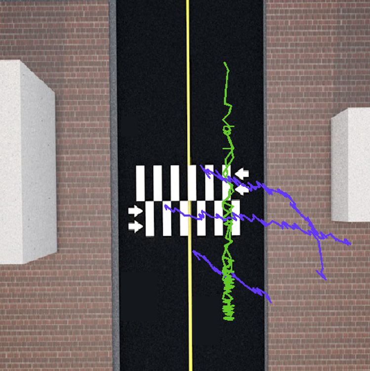
Appl. Sci. 2020, 10, 1057 3 of 21
Appl. Sci. 2020, 10, x FOR PEER REVIEW 3 of 21
Appl. Sci. 2020, 10, x FOR PEER REVIEW 3 of 21
(a) (b)
Figure 1.
Figure (a)
Closed-circuit
1. Closed-circuit television (CCTV)
television (CCTV) views
views in
in (a)
(a) spot
spot A; (b) (b)
A; and
and (b) spot
spot B.
B.
Figure 1. Closed-circuit television (CCTV) views in (a) spot A; and (b) spot B.
All videos
All videosframesframeswere were handled
handled locally on aon
locally server we deployed
a server in the Osan
we deployed in theSmartOsanCitySmart
Integrated
City
Operations
Integrated Center.
Operations
All videos Since
frames these
Center. areas
were Since
handled are
these located
areason
locally near schools
arealocated
server we and residential
neardeployed
schools and complexes,
in theresidential
Osan Smartthe “floating
complexes,
City
population”
theIntegrated passing through
“floating Operations
population” Center. these
passing Since areas
theseisthese
through highest
areas are
areasduring
located commuting
near
is highest schools hours.
and
during commuting Thus,hours.
residential we used
complexes,
Thus, video
we
footage
used recorded
the video
“floating
footage between
population”
recorded 8 am
passing and
between 9 8am
through on
amtheseweekdays.
and areas
9 amison We extracted
highest duringWe
weekdays. only
commuting video
extracted clipsThus,
hours.
only containing
video we
clips
scenes
used where
containingvideo at least
footage
scenes where oneatpedestrian
recordedleastbetween and8 am
one pedestrian oneand
car
and9were
amoneonsimultaneously
weekdays.
car We in camera
extracted
were simultaneously view.
inonly Asview.
video
camera aclips
result,
As
we processed
containing 429
scenes and 359
where video
at leastclips
one of potential
pedestrian vehicle–pedestrian
and one car were interaction
simultaneously
a result, we processed 429 and 359 video clips of potential vehicle–pedestrian interaction events events
in camerain spots
view. AAsand
in
B, arespectively.
spots result,
A andwe B, processed
Frame sizes
respectively. 429 Frame
and 359
of the video
obtained
sizes clips
of the of potential
video
obtained arevehicle–pedestrian
clipsvideo clips×are
1280 7201280
pixels
× 720interaction
at both atevents
pixelsspots, bothand inhad
spots,
andspots
been had Abeen
and B,
recorded atrespectively.
15 andat1115fps
recorded Frame
and 11sizes of the obtained
(frames-per-second),
fps (frames-per-second), video clips
respectively. are
Due1280
respectively.to ×privacy
720 pixels
Due at both
issues,
to privacy we spots,
viewed
issues, we
and
viewed had
the processed been recorded
trajectory
the processed at 15 and
data only
trajectory 11 fps
after
data (frames-per-second),
onlyremoving the original
after removing respectively. Due
videos. Figure
the original to privacy
videos. 2Figure issues,
represents we A
spots
2 represents
andviewed
BAwith the processed trajectoryand datacrosswalks
only after fromremoving the original videos. Figure as well2as represents
spots andthe roads,the
B with sidewalks,
roads, sidewalks, and crosswalks an overhead
from an perspective,
overhead perspective, illustrating
as well as
a spots
sample A and
of B
objectwith the roads,
trajectories sidewalks,
which and
resulted crosswalks
from our from an
processing. overhead
Blue perspective,
and green as well
lines as
indicate
illustrating a sample of object trajectories which resulted from our processing. Blue and green lines
illustratingand
pedestrians a sample
vehicles,of object trajectories which resulted from our processing. Blue and green lines
respectively.
indicate pedestrians and vehicles, respectively.
indicate pedestrians and vehicles, respectively.
(a) (b)
(a) (b)
Figure2.2.Diagrams
Figure Diagramsof
of objects’
objects’ trajectories
trajectories in
in(a)
(a)spot
spotA;
A;and
and(b)
(b)spot
spotBB
inin
overhead view.
overhead view.
Figure 2. Diagrams of objects’ trajectories in (a) spot A; and (b) spot B in overhead view.
2.2. Proposed
2.2. ProposedPPRE
PPREAnalysis
AnalysisSystem
System
2.2. Proposed PPRE Analysis System
InIn thissection,
this section,wewepropose
proposeaasystem
system which
which can
can analyze
analyzepotential
potentialpedestrian
pedestrian risky events
risky eventsusing
using
In this
various section, we
traffic-related propose
objects’ a system
behavioralwhich can
features. analyze
Figure potential pedestrian
3 illustrates the overall risky events
structure. using
The
various traffic-related objects’ behavioral features. Figure 3 illustrates the overall structure. The system
various
systemtraffic-related objects’ behavioral features. (2)
Figure 3 illustrates the overall and
structure. The
consists ofconsists of three
three modules: modules: (1) Preprocessing,
(1) Preprocessing, behavioral
(2) behavioral feature feature extraction,
extraction, and (3) PPRE(3) analysis.
PPRE
system consists of three modules: (1) Preprocessing, (2) behavioral feature extraction, and
analysis. In the first module, traffic-related objects are detected from the video footage using the mask (3) PPRE
analysis.
R-CNNIn(regional
the first convolutional
module, traffic-related objectsmodel,
neural network) are detected from thedeep
a widely-used video footagealgorithm.
learning using theWemask
R-CNN (regional convolutional neural network) model, a widely-used deep learning algorithm. We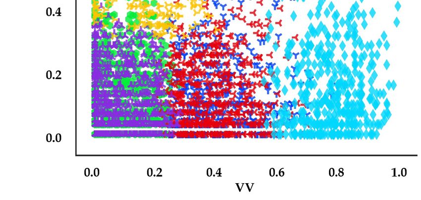
Appl. Sci. 2020, 10, 1057 4 of 21
Appl. Sci. 2020, 10, x FOR PEER REVIEW 4 of 21
In the first module, traffic-related objects are detected from the video footage using the mask R-CNN
first capture the “ground tip” point of each object, which are the points on the ground directly
(regional convolutional neural network) model, a widely-used deep learning algorithm. We first
underneath the front center of the object in oblique view. These ground tip points are then
capture the “ground tip” point of each object, which are the points on the ground directly underneath
transformed into the overhead perspective, with the obtained information being delivered to the next
the front center of the object in oblique view. These ground tip points are then transformed into the
module.
overhead perspective, with the obtained information being delivered to the next module.
Figure 3. Overall architecture of the proposed analysis system.
Figure 3. Overall architecture of the proposed analysis system.
InInthe
thesecond
secondmodule,
module,wewe extract
extract various
various features
features frame-by-frame,
frame-by-frame,such as as
such vehicle velocity,
vehicle velocity,
vehicle acceleration, pedestrian velocity, the distance between vehicle and pedestrian,
vehicle acceleration, pedestrian velocity, the distance between vehicle and pedestrian, and the and the
distance
distance between vehicle and crosswalk. In order to obtain objects’ behavioral features, it is important
between vehicle and crosswalk. In order to obtain objects’ behavioral features, it is important to
to obtain the trajectories of each object. Thus, we apply a simple tracking algorithm through the use
obtain the trajectories of each object. Thus, we apply a simple tracking algorithm through the use
of threshold and minimum distance methods, and then extract their behavioral features. In the last
of threshold and minimum distance methods, and then extract their behavioral features. In the last
module, we analyze the relationships between the extracted object features through data mining
module, we analyze the relationships between the extracted object features through data mining
techniques such as k-means clustering and decision tree methodologies. Furthermore, we describe
techniques such as k-means clustering and decision tree methodologies. Furthermore, we describe
the means of each cluster, and discuss the rules of the decision tree and explain how these statistical
themethods
means of each cluster,
strengthen and discuss
the analysis the rules of the decision
of pedestrian–automobile tree and explain how these statistical
interactions.
methods strengthen the analysis of pedestrian–automobile interactions.
2.3. Preprocessing
2.3. Preprocessing
This section briefly describes how we capture the “contact points” of traffic-related objects such
This section
as vehicles and briefly describes
pedestrians. how we
A contact capture
point the “contact
is a reference pointpoints”
we assignof traffic-related
to each object toobjects such as
determine
vehicles and pedestrians.
its velocity and distance A contact
from otherpoint is aTypical
objects. reference point
video we assign
footage to each
extracted fromobject
CCTVtoare determine
captured its
velocity
in oblique view, since the cameras are installed at an angle from the view area, so the contact captured
and distance from other objects. Typical video footage extracted from CCTV are points
in of
oblique view,depends
each object since theon cameras are installed
the camera’s angle asatwell
an angle from the view
as its trajectory. Thus,area, so the
we need tocontact
convertpoints
the
of contact
each object
points depends on thetocamera’s
from oblique overheadangle as welltoas
perspective its trajectory.
correctly Thus,the
understand we need to
objects’ convert the
behaviors.
contactThis
points
is afrom oblique
recurring to overhead
problem in trafficperspective
analysis that toothers
correctly
haveunderstand theIn
tried to solve. objects’ behaviors.
one case, Sochor
et This
al. proposed a model
is a recurring problemconstructing 3-D bounding
in traffic analysis boxes
that others havearound
tried tovehicles
solve. Inthrough
one case,the use of
Sochor et al.
convolutional
proposed a model neural networks3-D
constructing (CNNs)
boundingfrom boxes
only a around
single camera
vehiclesviewpoint. Thisuse
through the makes it possible
of convolutional
to project
neural the coordinates
networks (CNNs) from of the car afrom
only an oblique
single camera viewpoint
viewpoint.toThisdimensionally-accurate
makes it possible to space [16].the
project
Likewise, Hussein et al. tracked pedestrians from two hours of video data
coordinates of the car from an oblique viewpoint to dimensionally-accurate space [16]. Likewise, from a major signalized
Appl. Sci. 2020, 10, 1057 5 of 21
Appl. Sci. 2020, 10, x FOR PEER REVIEW 5 of 21
Hussein et al.intracked
intersection New York pedestrians fromThe
City [17]. twostudy
hours used
of video an data from a major
automated videosignalized
handling intersection
system set in to
New York City [17]. The study used an automated video handling
calibrate the image into an overhead view, and then tracked the pedestrians using computer system set to calibrate the image
vision
into an overhead
techniques. These view,
twoand then tracked
studies appliedthe pedestrians
complex using computer
algorithms or multiplevision techniques.
sensors These two
to automatically
studies applied complex algorithms or multiple sensors to automatically
obtain objects’ behavioral features, but, in practice, these approaches require high computational obtain objects’ behavioral
features,
power, and but,arein difficult
practice,tothese
expandapproaches
to a largerrequire
urbanhigh computational
scale. Therefore, it power, and are
is still useful todifficult
developtoa
expand
simpler to a largerfor
algorithm urban scale. Therefore,
the processing of videoit data.
is still useful to develop a simpler algorithm for the
processing of video data.
First, we used a pre-trained mask R-CNN model to detect and segment the objects in each frame.
First, R-CNN
The mask we usedmodel a pre-trained mask R-CNN
is an extension of the model to detectmodel,
faster R-CNN and segment the objects
and it provides theinoutput
each frame.
in the
The
form of a bitmap mask with bounding-boxes [18]. Currently, deep-learning algorithms in the fieldthe
mask R-CNN model is an extension of the faster R-CNN model, and it provides the output in of
form of a bitmap
computer vision mask with bounding-boxes
have encouraged [18]. Currently,
the development of object deep-learning
detection and algorithms in the field of
instance segmentation
computer vision have
[19]. In particular, encouraged
faster R-CNN models the development
have beenof object detection
commonly used toand instance
detect segmentation
and segment objects[19].
in
In particular, faster R-CNN models have been commonly used to detect
image frames, with the only output being a bounding-box [20]. However, since the proposed system and segment objects in image
frames,
estimates with
thethe only output
contact point being a bounding-box
of objects through the [20].
useHowever, since the proposed
of a segmentation mask over system
the estimates
region of
the contact
interest point
(RoI) in of objects through
combination withthetheusebounding-box,
of a segmentation we mask
used over the region
the mask R-CNN of interest
model(RoI) in
in our
combination
experiment [21]. with the bounding-box, we used the mask R-CNN model in our experiment [21].
In
In our
our experiment,
experiment, we we applied
applied object
object detection
detection APIAPI (application
(application programming
programming interface)
interface) within
within
the Tensorflow platform. The pre-trained mask R-CNN model is RestNet-101-FPN,
the Tensorflow platform. The pre-trained mask R-CNN model is RestNet-101-FPN, which is provided which is provided
by
by Microsoft
Microsoft common
common objects
objects in in the
the context
context (MS(MS COCO)
COCO) image image dataset
dataset [22,23].
[22,23]. Our
Our target
target objects
objects
consisted
consisted only
onlyofofvehicles
vehiclesand andpedestrians,
pedestrians, which waswas
which accomplished
accomplished withwith
aboutabout99.9%99.9%
accuracy. Thus,
accuracy.
no additional model training was needed for our
Thus, no additional model training was needed for our purposes. purposes.
Second,
Second, we we aimed
aimed to to capture
capture thethe ground
ground tip tip points
points of of vehicles
vehicles and pedestrians, which
and pedestrians, which are are located
located
directly under the
directly under the center
centerofofthe thefront
frontbumper
bumper and
and ononthethe ground
ground between
between the the
feet,feet, respectively.
respectively. For
For vehicles, we captured the ground tip by using the object mask and central
vehicles, we captured the ground tip by using the object mask and central axis line of the vehicle lane, axis line of the vehicle
lane,
and aandmorea more detailed
detailed procedure
procedure for for
thisthis is described
is described in in
ourour previousstudy,
previous study,[24].[24].WeWe used
used aa similar
similar
procedure
procedure for pedestrians, and as seen in Figure 4, we regarded the midpoint from their tiptoe points
for pedestrians, and as seen in Figure 4, we regarded the midpoint from their tiptoe points
within
within mask,
mask, as as the
the ground
ground tip tip point.
point.
Figure 4. Ground point of pedestrian for recognizing its
its overhead
overhead view
view point.
point.
Next,
Next, with
with the
the recognized
recognized ground
ground tip
tip points,
points, we
we transformed
transformed themthem into
into an
an overhead
overhead perspective
perspective
using
using the “transformation matrix” within the OpenCV library. The transformation matrix
the “transformation matrix” within the OpenCV library. The transformation matrix can
can be
be
derived
derived from
from four
four pairs
pairs of
of corresponding
corresponding “anchor
“anchor points”
points” in
in real
real image
image (oblique
(oblique view)
view) and
and virtual
virtual
space
space (overhead
(overheadview). Figure
view). 5 represents
Figure the anchor
5 represents points as
the anchor green as
points points frompoints
green the two perspectives.
from the two
In our experiment, we used the four corners of the rectangular crosswalk area as
perspectives. In our experiment, we used the four corners of the rectangular crosswalk area as anchor anchor points.
We measured
points. the real the
We measured length
realand width
length andofwidth
the crosswalk area on-site,
of the crosswalk then reconstructed
area on-site, it in virtual
then reconstructed it in
space
virtual space from an overhead perspective with proportional dimensions, oriented orthogonallyx–y
from an overhead perspective with proportional dimensions, oriented orthogonally to the to
plane.
the x–yWe then identified
plane. the vertex coordinates
We then identified of the rectangular
the vertex coordinates of the crosswalk
rectangulararea in the camera
crosswalk area image
in the
and the corresponding
camera image and the vertices in our virtual
corresponding verticesspace, andvirtual
in our used these
space,toand
initialize
used the OpenCV
these function
to initialize the
OpenCV function to apply to all detected contact points. A similar procedure for perspective
transformation is also described in detail in [24].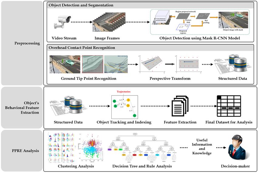
Appl. Sci. 2020, 10, 1057 6 of 21
to apply to all detected contact points. A similar procedure for perspective transformation is also
described in detail in [24].
Appl.
Appl. Sci.
Sci. 2020,
2020, 10,
10, xx FOR
FOR PEER
PEER REVIEW
REVIEW 66 of
of 21
21
(a)
(a) (b)
(b)
Figure
Figure5.5.
Figure Example
5.Example of
Exampleof perspective
ofperspective transform
perspectivetransform from
transformfrom (a)
from(a) oblique
(a)oblique view;
obliqueview; into
view;into (b)
into(b) overhead
(b)overhead view.
overheadview.
view.
2.4.
2.4.Object
2.4. ObjectBehavioral
Object BehavioralFeature
Behavioral FeatureExtraction
Feature Extraction
Extraction
In
Inthis
In thissection,
this section,we
section, wedescribe
we describehow
describe howto
how toextract
to extractthe
extract theobjects’
the objects’behavioral
objects’ behavioralfeatures
behavioral featuresfrom
features fromthe
from therecognized
the recognized
recognized
overhead
overhead contact
overhead contact point.
contact point. Vehicles
point. Vehicles
Vehicles andand pedestrians
and pedestrians
pedestrians existexist
exist as as contact
as contact points
contact points
points in in each
in each individual
each individual
individual frame.frame.
frame. To
To
To estimate
estimate velocity
estimate velocity
velocity andand acceleration,
and acceleration,
acceleration, we we must
we must identify
must identify each
identify each object
each object in
object in successive
in successive frames
successive frames and
frames and link
and link them
link them
them
into
intotrajectories.
into trajectories. The
trajectories. The field
The field of
field ofcomputer
of computervision
computer visionhas
vision hasdeveloped
has developedmany
developed manysuccessful
many successfulstrategies
successful strategiesfor
strategies forobject
for object
object
tracking
tracking[25–27].
tracking [25–27]. In
[25–27]. Inthis
In thisstudy,
this study,we
study, weapplied
we appliedaaasimple
applied simpleand
simple andlow-computational
and low-computationaltracking
low-computational trackingand
tracking andindexing
and indexing
indexing
algorithm,
algorithm, since
algorithm, since most
since most unsignalized
most unsignalized crosswalks
unsignalized crosswalks are
crosswalks areon narrow
are on
on narrowroads
narrow roadswith light
roads with pedestrian
with light pedestrian[25,27].
traffic
light pedestrian traffic
traffic
The algorithm
[25,27].
[25,27]. The identifies
The algorithm
algorithm each individual
identifies
identifies each object in
each individual
individual consecutive
object
object in framesframes
in consecutive
consecutive by using
frames by the threshold
by using
using the and
the threshold
threshold
minimum
and
and minimum distances
minimum distances of objects.
distances of For
of objects.example,
objects. For assume
For example, that
example, assume there
assume thatare three
that there detected
there areare three object (pedestrian)
three detected
detected object
object
positions in the
(pedestrian)
(pedestrian) first frame
positions
positions in named
in the
the firstA,
first B, and
frame
frame C, and
named
named A,in
A, B,the
B, andsecond
and C, andframe
C, and in thenamed
in the secondD,
second E, and
frame
frame F, respectively
named
named D,
D, E,
E, and
and
(see
F, Figure 6). (see
F, respectively
respectively (see Figure
Figure 6).
6).
Figure
Figure 6.Example
Figure6.6. Exampleof
Example ofobject
of objectpositions
object positionsin
positions intwo
in twoconsecutive
two consecutiveframes.
consecutive frames.
frames.
There
There are multiple object positions defined as x–y coordinates (contact points) in each frame,
There areare multiple
multiple object
object positions
positions defined
defined as as x–y
x–y coordinates
coordinates (contact
(contact points)
points) in in each
each frame,
frame,
and
and each object has a unique identifier (ID) ordered by detection accuracy. In Figure 6, A and B in the
and each
each object
object has
has aa unique
unique identifier
identifier (ID)
(ID) ordered
ordered byby detection
detection accuracy.
accuracy. In
In Figure
Figure 6,6, AA and
and BB in
in the
the
first
firstframe move to E and F in the second frame, respectively. C moves to somewhere out-of-frame,
first frame
frame move
move to to EE and
and FF in
in the
the second
second frame,
frame, respectively.
respectively. C C moves
moves toto somewhere
somewhere out-of-frame,
out-of-frame,
while
while D emerges in the second frame.
while D D emerges
emerges in in the
the second
second frame.
frame.
To
To ascertain
ascertain thethe trajectories
trajectories of
of each
each object,
object, we
we set
set frame-to-frame
frame-to-frame distance
distance thresholds
thresholds for for vehicles
vehicles
and
and pedestrians,
pedestrians, andand then
then compare
compare allall distances
distances between
between positions
positions from
from the
the first
first to
to the
the second
second frame,
frame,
as
as seen
seen inin Table
Table 1. 1. In
In this
this example,
example, ifif we
we set
set the
the pedestrian
pedestrian threshold
threshold at
at 3.5,
3.5, C C is
is too
too far
far from
from either
either
position
position in in the
the second,
second, but but within
within range
range ofof the
the edge
edge ofof the
the frame.
frame. When
When A A is
is compared
compared with with D,
D, E,
E, and
and
F, it is closest to E; likewise, B is closest to F. We can infer that A moved to E, and B moved to F, while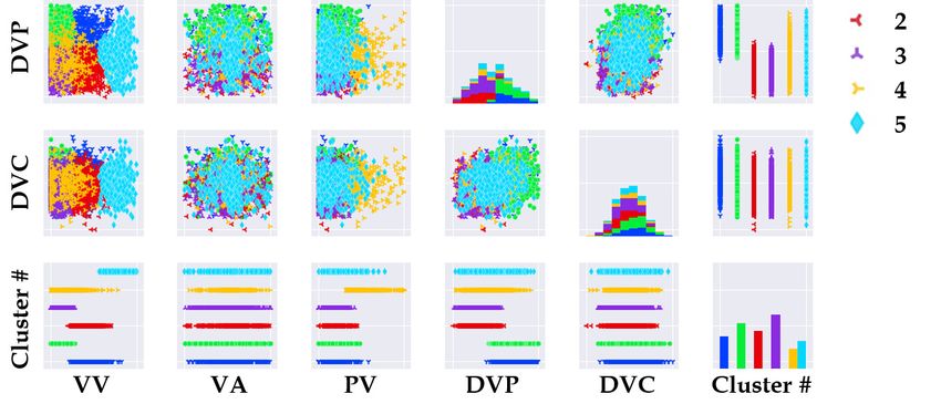
Appl. Sci. 2020, 10, 1057                                                                               7 of 21

       To ascertain the trajectories of each object, we set frame-to-frame distance thresholds for vehicles
and pedestrians, and then compare all distances between positions from the first to the second frame,
as seen in Table 1. In this example, if we set the pedestrian threshold at 3.5, C is too far from either
position in the second, but within range of the edge of the frame. When A is compared with D, E, and
F, it is closest to E; likewise, B is closest to F. We can infer that A moved to E, and B moved to F, while
a pedestrian at C left the frame, and D entered the frame. We apply this algorithm to each pair of
consecutive frames in the dataset to rebuild the full trajectory of each object.

            Table 1. Result of tracking and indexing algorithm using threshold and minimum distance.

        Object ID in First Frame     Object ID in Second Frame         Distance (m)        Result
                      A                           D                         4.518      Over threshold
                      A                           E                         1.651        Min. dist.
                      A                           F                         2.310
                      B                           D                         3.286
                      B                           E                         2.587
                      B                           F                         1.149        Min. dist.
                      C                           D                         7.241      Over threshold
                      C                           E                         5.612      Over threshold
                      C                           F                         3.771      Over threshold

      With the trajectories of these objects, we can extract the object’s behavioral features which affect
the potential risk. At each frame, we extracted five behavioral features for each object: Vehicle velocity
(VV), vehicle acceleration (VA), pedestrian velocity (PV), distance between vehicle and pedestrian
(DVP), and distance between vehicle and crosswalk (DVC). The extracting methods are described
below in detail.
      Vehicle and pedestrian velocity (VV and PV): In general, object velocity is a basic measurement
that can signal the likelihood of potentially dangerous situations. The speed limit in our testbed,
spots A and B, is 30 km/h, so if there are many vehicles detected driving over this limit at any point,
this contributes to the risk of that location. Pedestrian velocity alone is not an obvious factor for risk,
but when analyzed together with other features, we may find important correlations and interactions
between the object velocities and the likelihood for pedestrian risk.
      Velocity of objects is calculated by dividing an object’s distance moving between frames by the time
interval between the frames. In our experiment, videos were recorded at 15 and 11 fps in spots A and B,
respectively, and sampled at every fifth frame. Therefore, the time interval F between two consecutive
frames was 1/3 s in spot A, and 5/11 s, in spot B. Meanwhile, pixel distance in our transformed overhead
points was converted into real-world distance in meters. We infer pixel-per-meter constant (P) using
the actual length of the crosswalks as our reference point. In our experiment, the actual length of both
crosswalks in spots A and B were 15 m, and the pixel lengths of these crosswalks were 960 pixels. Thus,
object velocity was calculated as:

                                                     ob ject distance
                                        Velocity =                    m/s                                  (1)
                                                           F∗P
      The unit is finally converted into km/h.
      Vehicle acceleration (VA): Vehicle acceleration is also an important factor to determine the potential
risk for pedestrian injury. In general, while vehicles pass over a crosswalk with a pedestrian nearby,
they reduce speed (resulting in negative acceleration values). If many vehicles maintain speed (zero
value) or accelerate (positive values) while nearby the crosswalk or pedestrian, it can be considered as
a risky situation for pedestrians.
Appl. Sci. 2020, 10, 1057 8 of 21
Vehicle acceleration is the difference between vehicle velocities in the current frame (v0 ) and in the
next frame (v):
v − v0
Acceleration = m/s2 (2)
F
The unit is finally converted into km/h2 .
Distance between vehicle and pedestrian (DVP): This feature refers to the physical distance
between each vehicle and pedestrian. In general, if this distance is short, the driver should slow
down with additional caution. However, if the vehicle has already passed the pedestrian, accelerating
presents less risk than when the pedestrian ahead of the car. Therefore, we measure DVP to distinguish
between these types of situations. If a pedestrian is ahead of the vehicle, the distance has a positive
sign, if not, it has a negative sign:
object distance
+
P (m), i f the pedestrian is in f ront o f the vehicle
DVP = object distance (3)
−
P (m), otherwise
Distance between vehicle and crosswalk (DVC): This feature is also extracted by calculating the
distance between vehicle and crosswalk. We measure this distance from the crosswalk line closest to
the vehicle; when vehicle is on the crosswalk, the distance is 0:
ob ject distance
(m), i f a vehicle is out o f crosswalk
DVC = P (4)
0, otherwise
As a result of feature extraction, we can obtain a structured dataset suitable for various data
mining techniques, as seen in Table 2.
Table 2. Example of the structured dataset for analysis.
Spot # Event # Frame # VV (km/h) VA (km/h2 ) PV (km/h) DVP (m) DVC (m)
1 1 1 19.3 5.0 3.2 12.1 8.3
1 1 2 16.6 −2.1 2.9 −11.4 6.2
...
1 529 8 32.1 8.4 4.1 8.0 0
2 1 1 11.8 1.2 3.3 17.2 18.3
2 1 2 9.5 0.3 2.7 7.8 4.3
...
2 333 12 22.3 1.6 7.2 3.3 2.3
... : It means that the records are still listed
2.5. Data Mining Techniques for PPRE Analysis
In this section, we describe two data mining techniques used to elicit useful information for
an in-depth understanding of potential pedestrian risky events: K-means clustering and decision
tree methods.
K-means clustering: Clustering techniques consist of unsupervised and semi-supervised learning
methods and are mainly used to handle the associations of some characteristic features [28]. In this
study, we considered each frame with its extracted features as a record, and used k-means clustering to
classify them into categories which could indicate degrees of risk. The basic idea of k-means clustering
is to classify the dataset D into K different clusters, with the classified clusters Ci consisting of the
elements (records or frames) denoted as x. The set of elements between classified clusters is disjointed,
and the number of elements in each cluster Ci is denoted by ni . The k-means algorithm consists of
two steps [29]. First, the initial centroids for each cluster are chosen randomly, then each point in
the dataset is assigned to its nearest centroid by Euclidean distance [30]. After the first assignment,
each cluster’s centroid is recalculated for its assigned points. Then, we alternate between reassigning
Appl. Sci. 2020, 10, 1057                                                                                 9 of 21

points to the cluster of its closest centroid, and recalculating those centroids. This process continues
until the clusters no longer differ between two consecutive iterations [31].
     In order to evaluate the results of k-means clustering, we used the elbow method with the sum of
squared errors (SSE). SSE is the sum of squared differences between each observation and mean of its
group. It can be used as a measure of variation within a cluster, and the SSE is calculated as follows:
                                                        n
                                                        X
                                                SSE =         (xi − x)2                                      (5)
                                                        i=1

where n is the number of observations xi , which is a value of the i-th observation, and x is the mean of
all the observations.
      We ran k-means clustering on the dataset for a certain range of values of K, and calculate the SSE
for each result. If the line chart of SSE plotted against K resembles an arm, then the “elbow” on the
arm represents a point of diminishing returns when increasing K. Therefore, with the elbow method,
we selected an optimal number of K clusters without overfitting our dataset. Then, we validated the
accuracy of our clustering by using the decision tree method.
      Decision tree: Decision trees are widely used to model classification processes [32,33]. It is one of
many supervised learning algorithms, and can effectively divide a dataset into smaller subsets [34].
It takes a set of classified data as input, and arranges the outputs into a tree structure composed of
nodes and branches.
      There are three types of nodes: (1) root node, (2) internal node, and (3) leaf node. Root nodes
represent a choice that will result in the subdivision of all records into two or more mutually exclusive
subsets. Internal nodes represent one of the possible choices available at that point in the tree structure.
Lastly, the leaf node, located at the end of the tree structure, represents the final result of a series of
decisions or events [35,36]. Since a decision tree model forms a hierarchical structure, each path from
the root node to leaf node via internal nodes represents a classification decision rule. These pathways
can be also described as “if-then” rules [36]. For example, “if condition 1 and condition 2 and . . . condition
k occur, then outcome j occurs.”
      In order to construct a decision tree model, it is important to split the data into subtrees by
applying criteria such as information gain and gain ratio. In our experiment, we applied the popular
C4.5 decision tree algorithm, an extended algorithm of ID3 that uses information gain as its attribute
selection measure. Information gain is based on the concept of entropy of information, referring to the
reduction of the weight of desired information, which then determines the importance of variables [35].
C4.5 decision tree algorithm selects the attribute of the highest information gain (minimum entropy) as
the test attribute of the current node. Information gain is calculated as follows:

                                                                          v
                                                                          X Dj
                            In f ormation Gain(D, A) = Entropy(D) −                     Entropy D j          (6)
                                                                                  |D|
                                                                          j=1

where D is a given data partition, and A n is the attribute    o (the extracted five features in our experiment).
D is split into v partitions (subsets) as D1 , D2 , . . . , D j . Entropy is calculated as follows:

                                                               C
                                                               X
                                           Entropy(D) = −            pi log2 pi                              (7)
                                                               i=1

                            |Ci, D |
where pi is derived from |D|         , and has non-zero probability that an arbitrary tuple in D belongs to
class (cluster, in our experiment) C. The attribute with the highest information gain is selected. In the
decision tree, entropy is a numerical measure of impurity, and is the expected value for information.
The decision tree is constructed to minimize impurity.
Appl. Sci. 2020, 10, 1057 10 of 21
Note that in order to minimize entropy, the decision tree is constructed to maximize information
gain. However, information gain is biased toward attributes with many outcomes, referred to as
multivalued attributes. To address this challenge, we used C4.5 with “gain ratio”. Unlike with
information gain, the split information value represents the potential information generated by
splitting the training dataset D into v partitions, corresponding to v outcomes on attribute A. Gain
ratio are used for split criteria and calculated as follows [37,38]:
In f ormation Gain(A)
GainRatio(A) = (8)
SplitIn f o(A)
v
X Dj D j
SplitIn f o(A) = − log2 (9)
|D| |D|
j=1
The attribute with the highest gain ratio will be chosen for splitting attributes.
In our experiment, there are two reasons for using the decision tree algorithm. First, we can
validate the result of the k-means clustering algorithm. Unlike k-means clustering, the performance
of the decision tree can be validated through its accuracy, precision, recall, and F1 score. Precision is
the ratio of positive classification to the classified results, and recall is the ratio of data successfully
classified in the input data [37,39].
TP
Precision = (10)
(TP + FP)
TP
Recall = (11)
(TP + FN )
(Precision ∗ Recall)
F1 score = 2 × (12)
(Precision + Recall)
where TP is true positive, FP is false positive, and FN is false negative.
Second, we can analyze the decision tree results in-depth, by treating them as a set of “if-then”
rules applying to every vehicle–pedestrian interaction at that location. At the end of Section 3, we will
discuss the results of the decision tree and confirm the feasibility and applicability of the proposed
PPRE analysis system by analyzing these rules.
3. Experiments and Results
3.1. Experimental Design
In this section, we describe the experimental design for k-means clustering and decision trees as
core methodologies for the proposed PPRE analysis system. First, we briefly explain the results of
data preprocessing and statistical methodologies. The total number of records (frames) is 4035 frames
(spot A: 2635 frames and spot B: 1400 frames). Through preprocessing, we removed outlier frames
based on extreme feature values, yielding 2291 and 987 frames, respectively. We then conducted [0, 1]
normalization on the features as follows:
di − min(d)
d̂i = (13)
max(d) − min(d)
Prior to the main analyses, we conducted statistical analyses such as histogram and correlation
analysis. Figure 7a–f illustrated histograms of all features and each feature, respectively. VV and
PV features are skewed low since almost all cars and pedestrians stopped or moved slowly in these
areas. Averages of VV and PV are at about 24.37 and 2.5 km/h, respectively. When considering speed
limits are 30 km/h in these spots, and the average person’s speed is approximately 4 km/h, these
are reasonable values. DVP (distance from vehicle to pedestrian) shows two local maxima: One for
pedestrians ahead of the car, and one for behind.Appl. Sci.
Appl. Sci. 2020,
2020, 10,
10,1057
x FOR PEER REVIEW 11of
11 of21
21
Appl. Sci. 2020, 10, x FOR PEER REVIEW 11 of 21
(a) (b) (c)
(a) (b) (c)
(d) (e) (f)
(d) 7. Histograms of (a) all features; (b)
Figure (e)VV; (c) VA; (d) PV; (e) DVP; and (f)(f)DVC.
Figure 7. Histograms
Histograms of
of (a)
(a) all
all features;
features; (b) VV; (c) VA; (d) PV;
VA; (d) PV; (e)
(e) DVP;
DVP; and
and (f)
(f) DVC.
DVC.
Next, we can study the relationships between each feature by performing correlation analysis.
Figure 8a,bwe
Next, represents
can studycorrelation matrices
the relationships in spots
between A and
each B. In
feature byspot A, we can
performing observe analysis.
correlation negative
analysis.
correlation between VV and DVP. This indicates that
Figure 8a,b represents correlation matrices in spots A and B. In spot A, vehicles tended
A, we to
we can move
can observequickly near
observe negative
negative
pedestrians,
correlation
correlation indicating
between
between VVVV a and
and dangerous
DVP.DVP. situation
This indicates
This forvehicles
that
indicates the
that pedestrian. In spot
tended totended
vehicles move to B,
quickly there
move is negative
nearquickly
pedestrians,
near
correlation
indicating a between
dangerous PV and
situation DVP,
for which
the could
pedestrian. be
In interpreted
spot B, there in
is two ways:
negative
pedestrians, indicating a dangerous situation for the pedestrian. In spot B, there is negative Pedestrians
correlation betweenmoved
PV
quickly
and DVP,towhich
correlation avoidcould
betweena near-miss
PV beand by an
interpreted
DVP, inapproaching
whichtwocould car,
ways:bePedestriansor pedestrians
interpreted moved
in two slowed
quickly
ways: down
avoid aornear-miss
toPedestrians stopped
moved
altogether
by an to
approachingwait for
car,the
or car to pass
pedestrians nearby.
slowed Since
down we
or extracted
stopped only
altogether
quickly to avoid a near-miss by an approaching car, or pedestrians slowed down or stopped video
to clips
wait containing
for the car scenes
to pass
where
nearby. at least
Since
altogether one pedestrian
we extracted
to wait for the car onlyand one
to video car were in the
clips containing
pass nearby. camera
Since we scenes view
where
extracted at the
onlyatvideosame
least one time, DVP
clipspedestrian and
containingand DVC
one
scenes
have
car
where positive
wereat in thecorrelation.
least camera
one view atand
pedestrian the one
samecartime, DVP
were andcamera
in the DVC haveviewpositive correlation.
at the same time, DVP and DVC
have positive correlation.
(a) (b)
(a)
Figure8.
Figure 8. Correlation
Correlation matrices
matrices in
in (a)
(a) spot
spot A;
A;and
and(b) spot(b)
(b)spot B.
B.
Figure 8. Correlation matrices in (a) spot A; and (b) spot B.Appl. Sci. 2020, 10, 1057 12 of 21
Appl. Sci. 2020, 10, x FOR PEER REVIEW 12 of 21
For our experiment, we conducted both quantitative
quantitative and qualitative
qualitative analyses.
analyses. In the quantitative
analysis, we
analysis, weperformed
performed k-means
k-means clustering
clustering to obtain
to obtain the optimal
the optimal numbernumber of (K).
of clusters clusters (K). Each
Each clustering
clustering experiment was evaluated by the SSE depending on K between 2 to 10,
experiment was evaluated by the SSE depending on K between 2 to 10, and through the elbow method, and through the
elbow
we method,
chose we chose
the optimal the optimal
K. Then, we usedK.theThen, we used
decision tree the decision
method tree method
to validate to validate
the classified the
dataset
classified
with dataset
a chosen withproportion
K. The a chosen K.ofThe proportion
training of data
and test training
wereand test data
at about 70%were
(2287at frames)
about 70%and(2287
30%
frames)
(991 and 30%
frames), (991 frames),
respectively. respectively.
In the qualitativeInanalysis,
the qualitative analysis,
we analyzed wefeature
each analyzedandeach feature and
its relationship
its relationship
with withfeatures
multiple other multiple
byother features
clustering by clustering
them. them. Then,
Then, we analyzed we analyzed
the rules the rules
derived from derived
the decision
from the decision tree and their implications for the behavior and
tree and their implications for the behavior and safety at the two sites. safety at the two sites.
3.2. Quantitative Analysis
In order to obtain the optimal number of clusters, K, we looked at the sum of squared errors
between the
the observations
observationsandandcentroids
centroidsinineach
each cluster
cluster byby adjusting
adjusting K from
K from 2 to210
to(see
10 (see Figure
Figure 9).
9). SSE
SSE decreases
decreases withwith
eacheach additional
additional cluster,
cluster, butbut whenconsidering
when consideringcomputational
computationaloverhead,
overhead, the
the curve
flattens at K =
= 6. Thus,
Thus, we
we set
set the
the optimal
optimal KK at
at 6,
6, which
which means
means that the five behavioral features could
be sufficiently classified
classified into
into six
six categories.
categories.
Figure 9.
Figure Sum of
9. Sum of squared
squared errors
errors with
with elbow
elbow method
method for
for finding optimal K.
finding optimal K.
As a result of this clustering method, we obtained the labels (i.e., classes or categories). Since this
As a result of this clustering method, we obtained the labels (i.e., classes or categories). Since this
is an unsupervised learning model, and since the elbow method is partly subjective, we need to ensure
is an unsupervised learning model, and since the elbow method is partly subjective, we need to
that the derived labels are well classified.
ensure that the derived labels are well classified.
Thus, with the chosen K, we performed the decision tree classifier as a supervised model, and
Thus, with the chosen K, we performed the decision tree classifier as a supervised model, and
used the following parameter options for learning process: a gain ratio for split criterion, max tree
used the following parameter options for learning process: a gain ratio for split criterion, max tree
depth of 5, and binary tree structure. As a result, Table 3 shows the confusion matrix, with the accuracy
depth of 5, and binary tree structure. As a result, Table 3 shows the confusion matrix, with the
remaining at 92.43%, and the average precision, recall, and F1-score all staying at 0.92.
accuracy remaining at 92.43%, and the average precision, recall, and F1-score all staying at 0.92.
Table 3. Confusion matrix.
Table 3. Confusion matrix.
Actual Class
Expected Expected Class Actual Class
Class 0 1 0 12 2 33 4 54 5
0 137 0 1 137 14 4 00 1 21 2
1 1 1 212 1 2120 0 88 1 01 0
2 7 0 156 5 2 3
2 7 3
0 0
156 6
7
5
240 1 0
2 3
3 0 4 7 0 36 4 240
6 75 01 0
4 0 5 3 4 04 7 06 2 75
96 0
5 4 0 7 0 2 96
Thus, with the k-means clustering and decision tree methods, we determined an optimal number
Thus, (6),
of clusters withand
theevaluated
k-means clustering and decision
the performance of thetree methods,
derived we determined an optimal number
clusters.
of clusters (6), and evaluated the performance of the derived clusters.Appl. Sci. 2020, 10, x1057
FOR PEER REVIEW 13 of 21
3.3. Qualitative Analysis
3.3. Qualitative Analysis
We scrutinized the distributions and relationships between each two features, and clarified the
meaning scrutinized
We of each clusterthe by distributions
matching each andcluster’s
relationships between
classification eachand
rules two thefeatures,
degree of and clarified
PPRE. This
the meaning of each cluster by matching each cluster’s classification rules and
section consists of three parts: (1) Boxplot analysis for single feature by cluster, (2) scatter analysis the degree of PPRE.
for
This section consists
two features, and (3)ofrulethree parts: by
analysis (1) decision
Boxplot analysis
tree. for single feature by cluster, (2) scatter analysis
for two features, and (3) rule analysis by decision tree.
First, we viewed
viewed the the boxplot
boxplotgrouped
groupedby bycluster,
cluster,asasillustrated
illustratedinin
Figure
Figure 10a–e,
10a–e,as as
distributions
distributions of
VV, VA,VA,
of VV, PV, PV,
DVP,DVP,and DVC
and DVC features, respectively.
features, In Figure
respectively. 10a, cluster
In Figure #5 is skewed
10a, cluster higher higher
#5 is skewed than others,
than
and thisand
others, would
thisdistinguish it from the
would distinguish others
it from theoverall.
others In FigureIn10b,e,
overall. most
Figure frames
10b,e, most are evenlyare
frames allocated
evenly
to each cluster,
allocated to each and a clearand
cluster, lineadoes
clearnot lineseem
doestonot
exist for to
seem their classification.
exist In Figure 10c,
for their classification. we can10c,
In Figure see
that
we canin cluster
see that#4,in
most frames
cluster #4, are
mostassociated
frames arewithassociated
high walking withspeed. In Figurespeed.
high walking 10d, cluster #0 and
In Figure #1
10d,
are skewed higher than others, and have similar means and deviations.
cluster #0 and #1 are skewed higher than others, and have similar means and deviations. Comprehensively, cluster #5
has high VV and low
Comprehensively, PV, and
cluster #5 hascluster
high VV #4 has
andlow
lowVV PV,and
andhigh PV.#4Cluster
cluster has low#0VV andand#1high
havePV.high DVP,
Cluster
but cluster
#0 and #0 has
#1 have highmoderate
DVP, butVV, and#0
cluster cluster #1 has low
has moderate VV,VV.andAs above#1results
cluster has low reveal,
VV. As partial
aboveclusters
results
have
reveal, distinguishable
partial clusters features. However, boxplot
have distinguishable analysis
features. only illustrates
However, boxplotaanalysis
single feature, limiting itsa
only illustrates
use in clearly
single feature,defining
limitingthe degrees
its use of PPRE.
in clearly defining the degrees of PPRE.
(a) (b)
(c) (d)
(e)
Figure
Figure 10.
10. Boxplots
Boxplots of
of (a)
(a) VV;
VV; (b)
(b) VA; DVP; and
VA; (c) PV; (d) DVP; and (e)
(e) DVC
DVC by
by clusters.
clusters.Appl. Sci. 2020, 10, 1057 14 of 21
Appl. Sci. 2020, 10, x FOR PEER REVIEW 14 of 21
Second,
Second, we
we performed
performedthethecorrelation
correlationanalysis
analysisbetween
betweentwo
twofeatures byby
features using scatter
using matrices
scatter as
matrices
illustrated in Figure 11. This figure describes the comprehensive results for labeled frames by hue
as illustrated in Figure 11. This figure describes the comprehensive results for labeled frames by hue and
correlations between
and correlations each each
between feature.
feature.
Figure 11. Result of correlation analysis using scatter matrices by clusters.
We studied three cases which are well-marked in detail (see Figure 12a–c). Figure 12a represents
the distributions between VV and PV features by cluster. Cluster #5 features high-speed cars and
slow pedestrians. This could be interpreted as moments when pedestrians walk slowly or stop to
wait for fast-moving cars to pass by. Cluster #4 could be similarly interpreted as moments when cars
stop or drive slowly to wait for pedestrians to quickly cross the street.
Figure 12b illustrates the scatterplot between VV and DVP features. Remarkably, most clusters
appear well-defined except for cluster #4. For example, cluster #3 has low VV and low DVP, for cars
slowing or stopped while near pedestrians. Cluster #2 has higher VV than those of cluster #3 and low
DVP, representing cars11.
Figure that
11. move
Result quickly while
of correlation analysisnear
usingpedestrians. Cluster
matrices
scatter matrices #5 seems to capture
by clusters.
by clusters.
vehicles traveling at high speeds regardless of their distance from pedestrians.
We
We studied
studied
Finally, three
Figurethree
12ccases
cases
showswhich
the are
which are well-marked
well-marked
relationships in
in detail
between PV(see
detail andFigure
(see DVP. 12a–c).
Figure 12a–c). Figure 12a
In this figure, represents
cluster #1 has
the
low distributions
the distributions between
PV and high DVP, between VV and PV features
VV andpedestrians
capturing PV features by cluster. Cluster
by cluster.
walking slowly #5
Cluster features high-speed
#5 features
even when far from and
cars
high-speed
cars are carsslow
them. and
In
pedestrians.
cluster This could
slow pedestrians.
#4, regardless bedistance
interpreted
Thisofcould as cars,
be interpreted
from moments when pedestrians
aspedestrians
moments when walk
to slowly
pedestrians
run quickly or stop to
walkapproaching
avoid slowly orwait
stop for
to
cars.
fast-moving
wait for cars
fast-moving to pass
carsby.
to Cluster
pass by. #4 could
Cluster #4be similarly
could be interpreted
similarly as moments
interpreted as when
moments
Through these analyses, it is possible to know features’ distributions as allocated to each cluster, and cars stop
when or
cars
drive
stop
to slowly
or
simply drive to
infer wait
slowly
the for pedestrians
to wait
type of thattoeach
quickly
for pedestrians
PPRE cross
to quickly
cluster thecross
street.
represents. the street.
Figure 12b illustrates the scatterplot between VV and DVP features. Remarkably, most clusters
appear well-defined except for cluster #4. For example, cluster #3 has low VV and low DVP, for cars
slowing or stopped while near pedestrians. Cluster #2 has higher VV than those of cluster #3 and low
DVP, representing cars that move quickly while near pedestrians. Cluster #5 seems to capture
vehicles traveling at high speeds regardless of their distance from pedestrians.
Finally, Figure 12c shows the relationships between PV and DVP. In this figure, cluster #1 has
low PV and high DVP, capturing pedestrians walking slowly even when cars are far from them. In
cluster #4, regardless of distance from cars, pedestrians run quickly to avoid approaching cars.
Through these analyses, it is possible to know features’ distributions as allocated to each cluster, and
to simply infer the type of PPRE that each cluster represents.
(a) (b) (c)
Figure
Figure12.
12.Cluster
Clusterdistributions
distributionsof
of(a)
(a)VV–PV;
VV–PV; (b)
(b) VV–DVP;
VV–DVP; and (c) PV–DVP.
PV–DVP.
Figure 12b
Finally, we illustrates
visualizedthe
thescatterplot
decision treebetween VV and it
and analyzed DVP features.
in order Remarkably,
to figure out howmost
eachclusters
cluster
appearbewell-defined
could matched to except
degrees forofcluster
PPRE.#4.NoteForthat
example, cluster tree
the decision #3 has low VV
makes and lowtoDVP,
it possible for cars
analyze the
slowing or stopped while near pedestrians. Cluster #2 has higher VV than those of cluster #3
classified frames in detail in the form of “if-then” rules. Figure 13 shows the result of the full decisionand low
DVP, representing cars that move quickly while near pedestrians. Cluster #5 seems to capture vehicles
traveling at high speeds regardless of their distance from pedestrians.
Finally, Figure 12c shows the relationships between PV and DVP. In this figure, cluster #1 has low
PV and high DVP, capturing pedestrians walking slowly even when cars are far from them. In cluster
#4, regardless of(a)
distance from cars, pedestrians run (b)
quickly to avoid approaching cars. (c)
Through these
analyses, it is possible to know
Figure 12. Clusterfeatures’ distributions
distributions as allocated
of (a) VV–PV; to each
(b) VV–DVP; and cluster, and to simply infer
(c) PV–DVP.
the type of PPRE that each cluster represents.
Finally, we visualized the decision tree and analyzed it in order to figure out how each cluster
could be matched to degrees of PPRE. Note that the decision tree makes it possible to analyze the
classified frames in detail in the form of “if-then” rules. Figure 13 shows the result of the full decisionYou can also read