Automated Location Matching in Movies
←
→
Page content transcription
If your browser does not render page correctly, please read the page content below
Automated Location Matching in Movies
F. Schaffalitzky1,2 and A. Zisserman2
1
Balliol College, University of Oxford
2
Robotics Research Group, University of Oxford, UK
{fsm,az}@robots.ox.ac.uk
Abstract. We describe progress in matching shots which are images of the same 3D loca-
tion in a film. The problem is hard because the camera viewpoint may change substantially
between shots, with consequent changes in the imaged appearance of the scene due to
foreshortening, scale changes, partial occlusion and lighting changes.
We develop and compare two methods which achieve this task. In the first method we
match key frames between shots using wide baseline matching techniques. The wide base-
line method represents each frame by a set of viewpoint covariant local features. The lo-
cal spatial support of the features means that segmentation of the frame (e.g. into fore-
ground/background) is not required, and partial occlusion is tolerated. Matching proceeds
through a series of stages starting with indexing based on a viewpoint invariant description
of the features, then employing semi-local constraints (such as spatial consistency) and
finally global constraints (such as epipolar geometry).
In the second method the temporal continuity within a shot is used to compute invariant
descriptors for tracked features, and these descriptors are the basic matching unit. The
temporal information increases both the signal to noise ratio of the data and the stability of
the computed features. We develop analogues of local spatial consistency, cross-correlation
and epipolar geometry for these tracks.
Results of matching shots for a number of very different scene types are illustrated on two
entire commercial films.
1 Introduction
The objective of this work is to establish matches between the various locations (3D scenes) that
occur throughout a feature length movie. Once this is achieved a movie can be browsed by, for
example, only watching scenes that occur on a particular “set” [4, 7] – such as all the scenes
that take place in Rick’s bar in “Casablanca”. Matching on location is a step towards enabling
a movie to be searched by visual content, and complements other search methods such as text
(from subtitles or voice recognition transcription) or matching on actor’s faces.
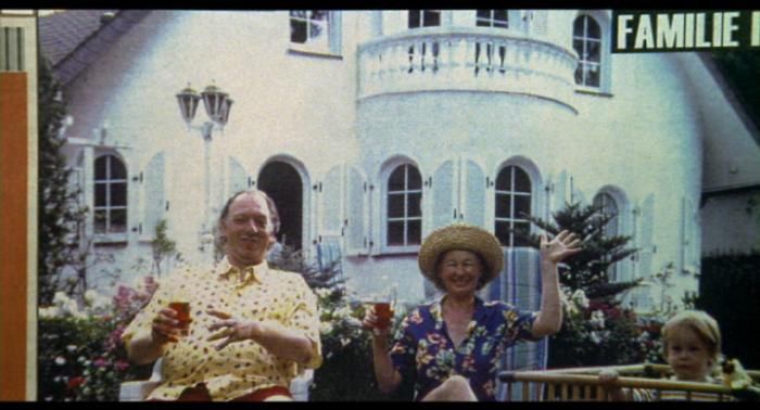
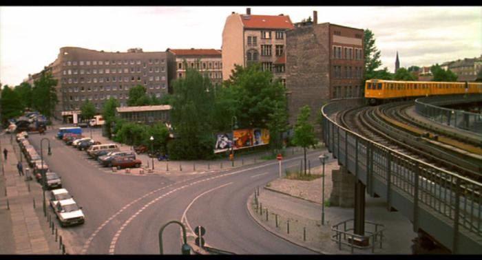
This is a very challenging problem: locations may be filmed under very different imaging
conditions including changes of lighting, scale and viewpoint. There is often also partial occlu-
sion by foreground objects (actors, vehicles). These problems are illustrated in figure 1. For such
cases a plethora of so called “wide baseline” methods have been developed, and this is still an
area of active research [2, 10–12, 15, 14, 17–20, 22, 24, 25, 27, 28]).
Here the question we wish to answer for each pair of shots is “Do these shots include com-
mon 3D locations?”. Shots are used because a film typically has 100–150K frames but only of
the order of a thousand shots, so the matching complexity is considerably reduced. However,
to date wide baseline methods have mainly been applied to a relatively small number of views
(usually two, but of the order of tens in [22]), so the task is two orders of magnitude greater
than the state of the art. Since this involves exploring a 1000 × 1000 shot matching matrix, we
make careful use of indexing and spatial consistency tests to reduce the cost of the potentially
quadratic complexity. The final outcome is a film’s shots partitioned into sub-sets corresponding
to the same location.

Fig. 1. These three images are acquired at the same 3D location but from very different viewpoints. The
affine distortion between the imaged sides of the tower is evident, as is the difference in brightness. There
is considerable foreground occlusion of the church, plus image rotation . . .

     We develop and compare two approaches. Both approaches are based on representing the
location by a set of viewpoint independent feature vectors as described in section 2. In the
first approach each shot is represented by a small number of independent key frames. Invariant
features descriptors are computed for these frames, and key frames are then matched using a set
of progressively stronger multiview constraints. The constraints capture the fact that not only
should the features match, but that the matches should be spatially consistent. This approach is
described in detail in section 3, and is similar to that of [22].
     Key frames only capture a limited part of a shot. An alternative is to compute descriptors
using all the contiguous frames within a shot. This is the basis of the second approach in which
viewpoint invariant features for individual frames are tracked throughout the shot. The temporal
continuity is used to improve the estimation of the invariant descriptors and to identify stable
features. We develop a second algorithm for shot matching based on these tracked features which
is described in section 4. This approach is entirely novel compared to [22] but follows naturally
from [21].
     The most closely related work to the shot matching is that of Aner and Kender [1], though
an earlier example is [3]. In [1] image mosaics are built for panning cameras and matched using
colour histograms for spatial blocks. However, the matching constraints are not rooted in the
fact that the scenes are 3D.
     The algorithms described here for each approach are designed with efficiency in mind and
use invariant indexing to avoid exhaustive search in matching between shots. In order to avoid a
combinatorial explosion the invariant descriptors must be sufficiently distinctive, and this is one
of the key issues investigated here. Different methods of achieving distinctive descriptors can be
employed in the key frame and complete shot cases.
We illustrate the method on two feature films: “Groundhog Day” [Ramis, 1993] and “Run
Lola Run” (“Lola Rennt”) [Tykwer, 1999]. These films are chosen because they are both ‘time
films’ – where the characters act out the same time sequences several times, but with minor or
major variations. This means that many more locations are returned to than in a typical film,
and so the matching matrix is denser. In both cases the film is first partitioned into shots using
standard methods (colour histograms and motion compensated cross-correlation [8]).

2 Invariant descriptors for multiview matching
In this section we describe the invariant descriptors which facilitate multiple view matches, i.e.
point correspondences over multiple images.
    We follow the, now standard, approach in the wide baseline literature and start from features
from which we can compute viewpoint invariant descriptors. The viewpoint transformations
we consider are an affine geometric transformation (which models viewpoint change locally),
x 7→ Ax + b where x, b are 2-vectors and A is a 2 × 2 matrix; and an affine photometric trans-
formation on the intensity (which models lighting change locally), I 7→ sI + t. The descriptors
are constructed to be unaffected by these classes of geometric and photometric transformation;
this is the meaning of invariance.
    Features are determined in two stages: first, image regions which transform covariantly with
viewpoint are detected in each frame, second, a vector of invariant descriptors is computed for
each region. The invariant vector is a label for that region, and will be used as an index into
an indexing structure for matching between frames — the corresponding region in other frames
will (ideally) have an identical vector.
    We use two types of feature: one based on interest point neighbourhoods, the other based on
the “Maximally Stable Extremal” (MSE) regions of Matas et al. [13]. In both types an elliptical
image region is used to compute the invariant descriptor. Both features are described in more
detail below. It is beneficial to have more than one type of feature because in some imaged
locations a particular type of feature may not occur at all.

Invariant interest point neighbourhoods: In each frame, Harris [5] interest points are com-
puted independently over several scales and the detection scale of each interest point is deemed
to be verified if it is a local extremum (across scale) for the Laplacian operator. This is the
method described in [16] and corrects for the effects of scale changes due to camera zoom or
motion. Next, the neighbourhood of the feature is affinely rectified in such a way as to maximize
the isotropy of the intensity gradient nearby, as described in [9, 2]. This step corrects for the
effects of foreshortening.
    In brief, the Harris interest operator at scale s > 0 works as follows. Given an intensity
image I(x, y), the partial derivatives Ix , Iy are computed by convolution with derivatives of a
2D isotropic Gaussian filter with width sσg . Next we form, at each pixel, the 2 × 2 matrix

                                                        Ix Ix Ix Iy
                               F(x, y) = ∇I ⊗ ∇I =
                                                        Ix Iy Iy Iy

which obviously has rank at most one. We then smooth this “matrix field” (by convolving each
of the scalar images Ix Ix , Ix Iy , Iy Iy separately) using another Gaussian filter of width sσi . The
result is a symmetric matrix M = M(x, y), at each position (x, y) of the image. It is a weighted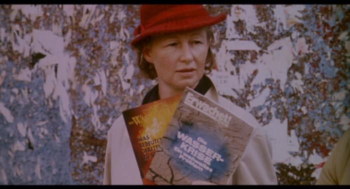
Fig. 2. Covariant region I. Invariant neighbourhood process, illustrated on details from the first and last
images from figure 1. In each case, the left image shows the original image and the right image shows
one of the detected feature points with its associated neighbourhood. Note that the ellipses are computed
independently in each image, but deform covariantly with the viewpoint to cover the same surface region
in both images.

form of the covariance matrix of the image intensity gradient around each point. It follows that
if there is no preferred or distinguished direction for image gradients near (x, y) then M will be
a scalar multiple of the identity matrix. On the other hand, if all the intensity gradients near
(x, y) are in the same direction then M will be close to having rank one. The Harris interest point
detector works by maximimizing the cornerness measure det M − 0.04(trace M) 2 over image
position (x, y). The affine adaptation works by searching, over unimodular (area preserving)
affine transformations of the image, for the affine rectification that maximizes the isotropy of the
rectified image. The idea is straightforward: if the point (x, y) has moment matrix M then, due
to the way that derivatives transform under affine rectification, the image should be transformed
by the matrix M1/2 , assuming that σg is negligible compared with σi . In practice this assumption
is not valid (in fact σg = 1.0 and σi = 1.6 in these experiments) and an iterative procedure is
needed: given an estimated rectification matrix A, rectify (warp) the image using A and compute
the moment matrix M of the warped image. Then update using Anew = M1/2 A and repeat till
convergence. This complication deals only with the issue of the shape of the support region of
the derivative operators. A real implementation would also need to use some damping in the
update and to test for cycles arising in the iteration. The image should be over-sampled to avoid
aliasing.
     The procedure is originally due to Baumberg [2], was also employed in [22], and is similar
to that of Mikolajczyk and Schmid [17].
     The outcome is an elliptical image region with the interest point as centre. The size of the el-
lipse is governed by the scale parameter s of the Laplacian operator at the extremum by choosing
the radius of the disk before affine rectification as 5 times the Laplacian scale. Figure 2 shows
an example of elliptical neighbourhoods detected independently in two views.
     For a 720 × 405 pixel video frame the number of neighbourhoods computed is typically
1600, but the number depends of course on the visual richness of the image. The computation
of the neighbourhood generally succeeds at points where there is signal variation in more than
one direction (e.g. near “blobs” or “corners”). It is possible for several neighbourhoods to have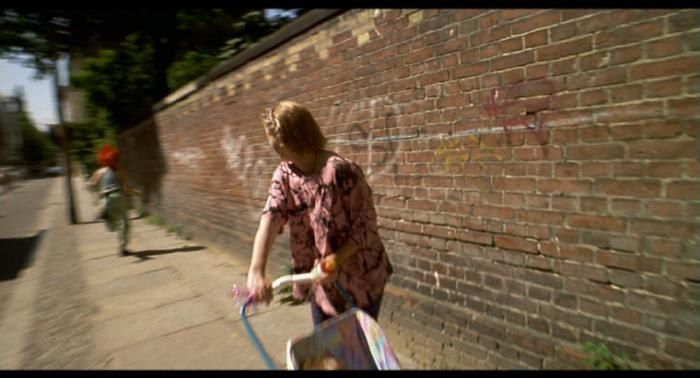
(virtually) the same centre, because there may be several characteristics scales for the same
interest point.

MSE regions: The regions are obtained by thresholding the intensity image and tracking the
connected components as the threshold value changes. A MSE region is declared when the area
of a component being tracked is approximately stationary. See figure 3 for an example. The idea
(and implementation used here) is due to Matas et al. [13]. Typically the regions correspond
to blobs of high contrast with respect to their surroundings such as a dark window on a grey
wall. Once the regions have been detected, the 2nd moments of the boundary of each region

Fig. 3. Covariant regions II. MSE (see main text) regions (outline shown in white) detected in images from
the data set illustrated by figure 1. The change of view point and difference in illumination are evident but
the same region has been detected in both images independently.

is computed and we construct an ellipse with the same 2nd moments. Finally, the regions are
replaced with elliptical regions twice the size of their associated 2nd moment ellipses. These
final regions are illustrated in figure 4.

Fig. 4. Example of covariant region detection. Left: frame number 40000 from “Run Lola Run”. Middle:
ellipses formed from 621 affine invariant interest points. Right: ellipses formed from 961 MSE regions.
Note the sheer number of regions detected just in a single frame and also the two types of region detectors
fire at different and complementary image locations.

Size of elliptical regions: In forming invariants from a feature, there is always a tradeoff be-
tween using a small intensity neighbourhood of the feature (which gives tolerance to occlusion)
and using a large neighbourhood (which gives discrimination). Since each type of feature gives
a family of nested elliptical regions (by scaling) we can address the problem by taking three
neighbourhoods (of relative sizes 1, 2, 3) of each feature and using all three in our image rep-
resentation. This idea has been formalized by Matas [15], who makes a distinction between the
region that a feature occupies in the image and the region (the measurement region) which one
derives from the feature in order to describe it. In our case, this means that the scale of detection
of a feature need not coincide with the scale of description.

                                                           Invariant 1


                                                                     Invariant 2


                                                                         Invariant 3

Fig. 5. Left and right: examples of corresponding features in two images. Each ellipse represents the de-
tected feature, so the nested ellipses are due to distinct features detected at different scales. Middle: Each
feature (shaded ellipse) gives rise to a set of derived covariant regions (unshaded ellipses). By choosing
a few (three) sizes of derived region one can tradeoff the distinctiveness of the regions against the risk of
hitting an occlusion boundary. Each size of region gives an invariant vector per feature.

Invariant descriptor: Given an elliptical image region which is co-variant with 2D affine trans-
formations of the image, we wish to compute a description which is invariant to such geometric
transformations and to 1D affine intensity transformations.
    Invariance to affine lighting changes is achieved simply by shifting the signal’s mean (taken
over the invariant neighbourhood) to zero and then normalizing its variance to unity.
    The first step in obtaining invariance to the geometric image transformation is to affinely
transform each neighbourhood by mapping it onto the unit disk. The process is canonical except
for a choice of rotation of the unit disk, so this device has reduced the problem from computing
affine invariants to computing rotational invariants. The idea was introduced by Baumberg in [2].
    The objective of invariant indexing is to reduce the cost of search by discarding match can-
didates whose invariants are different. While two very different features can have similar in-
variants, similar features cannot have very different invariants. Conceptually, the “distance” in
invariant space predicts a lower bound on the “distance” in feature space. Our invariant scheme
is designed so that Euclidean distance between invariant vectors actually (and not just con-
ceptually) provide a lower bound on the SSD difference between image patches. By contrast
Schmid [23] and Baumberg [2] both learn a distance metric in invariant space from training
data, which has the disadvantage of tuning the metric to the domain of training data.
    We apply a bank of linear filters, similar to derivatives of a Gaussian, and compute rotational
invariants from the filter responses. The filters used are derived from the family
                                Kmn (x, y) = (x + iy)m (x − iy)n G(x, y)

 where G(x, y) is a Gaussian. Under a rotation by an angle θ, the two complex quantities z =
x + iy and z̄ = x − iy transform as z 7→ eiθ z and z̄ 7→ e−iθ z̄, so the effect on Kmn is simply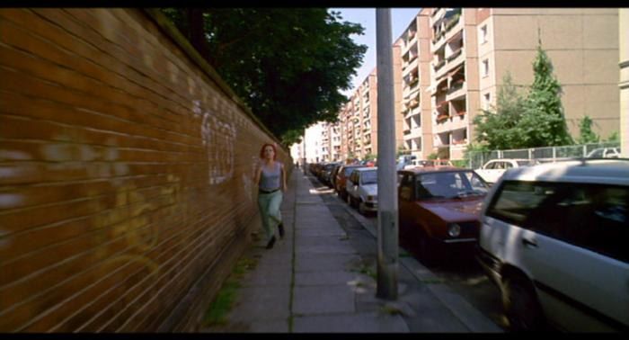
multiplication by ei(m−n)θ . Along the “diagonal” given by m − n = const the group action
is the same and filters from different “diagonals” are orthogonal so if we orthonormalize each
“diagonal” separately we arrive at a new filter bank with similar group action properties but
which is also orthonormal. This filter bank differs from a bank of Gaussian derivatives by a
linear coordinates change in filter response space. The advantage of our formulation is that the
group acts separately on each component of the filter response and does not “mix” them together,
which makes it easier to work with. Note that the group action does not affect the magnitude of
filter responses but only changes their relative phases. We used all the filters with m + n ≤ 6
and m ≥ n (swapping m nd n just gives complex conjugate filters) which gives a total of 16
complex filter responses per image patch.
     Taking the absolute value of each filter response gives 16 invariants. The inequality ||z| −
|w|| ≤ |z −w| guarantees (by Parseval’s theorem – the filter bank is orthonormal) that Euclidean
distance in invariant space is a lower bound on image SSD difference. Unfortunately, this ignores
the relative phase between the components of the signal.
     Alternatively, following [10, 16] one could estimate a gradient direction over the image patch
and artifically “rotate” each coefficient vector to have the same gradient direction. Instead, we
find, among the coefficients for with p = m − n 6= 0 the one with the largest absolute value
and artificially “rotate” the patch so as to make the phase 0 (i.e. the complex filter response is
real and positive). When p > 1 there are p ways to do this (p roots of unity) and we just put all
the p candidate invariant vectors into the index table. The property of distance in invariant space
being a lower bound on image SSD error is also approximately true for this invariant scheme,
the source of possible extra error coming from feature localization errors. The dimension of the
invariant space is 32.

Summary: We have constructed, for each invariant region, a feature vector which is invariant
to affine intensity and image transformations. Morever, the Euclidean distance between feature
vectors directly predicts a lower bound on the SSD distance between image patches, obviating
the need to learn this connection empirically.

3 Matching shots using key frames
In this section we sketch out the wide baseline approach to matching pairs of images. The
question we wish to answer is “Are these two images viewing the same scene or not?”. Our
measure of success is that we match shots of the same location but not shots of different 3D
locations. Shots are represented by key frames.
    The approach involves a number of steps, starting from local image descriptors which are
viewpoint invariant, progressing to the use of semi-local and finally global geometric constraints.
This order is principally due to efficiency considerations: the invariants are used within an in-
dexing structure. This is cheap (it involves only near-neighbour computations in the invariant
feature space) but there are many mismatches. A simple semi-local spatial consistency test re-
moves many of the mis-matches, and then a more expensive spatial consistency method is used
to accumuate more evidence for each surviving match. Finally, the most expensive and thorough
test is to verify that the matches satisfy the epipolar constraint. The various steps are described
in more detail below and are summarized in the algorithm of table 1.
    We will illustrate the method using key frames from shots 2 & 7, and 2 & 6 of figure 6, in
which one pair of frames is of the same scene, and the other is not. In ‘Run Lola Run’ there are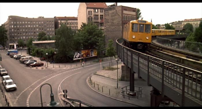
0                    1                    2                     3                    4

        18500                 19670                26000                27350                33900

           5                    6                    7                     8                    9

        52030                 53380                55800                56660                88300

Fig. 6. Ten test shots from the film “Run Lola Run” represented by key frames. The numbers above the key
frames gives the numbering of the shots which are selected in pairs corresponding to the same location.
The frame numbers are given below the key frames and these give an indication of the temporal position
of the shot within the film (which has a total of 115345 frames).

  1. Invariant descriptors for image features:
      (a) Detect features independently in each image.
     (b) In each image, compute a descriptor for each feature.
  2. Invariant indexing:
      (a) intra-image matching: Use invariant indexing to suppress indistinctive features, namely those
          that match six or more features in the same image.
     (b) inter-image matching: use invariant indexing of features descriptors to hypothesize matching
          features.
  3. Neighbourhood consensus: For each pair of matched features require that, among the K(= 10)
     nearest neighbours, N (= 1) are also matched.
  4. Local verification: Verify putatively matched features using intensity correlation.
  5. Semi-local and global verification: Use existing features matches to hypothesize new ones. Suppress
     ambiguous matches. Robustly fit epipolar geometry.

Table 1. Algorithm I: matching key frames with features. This is a simpler version of Algorithm II for
matching shots using feature tracks since the complications that arise from having feature tracks that extend
across multiple frames are absent. In outline the procedure is similar, though, progressing from invariant
feature descriptors through several stages of stronger matching criterion.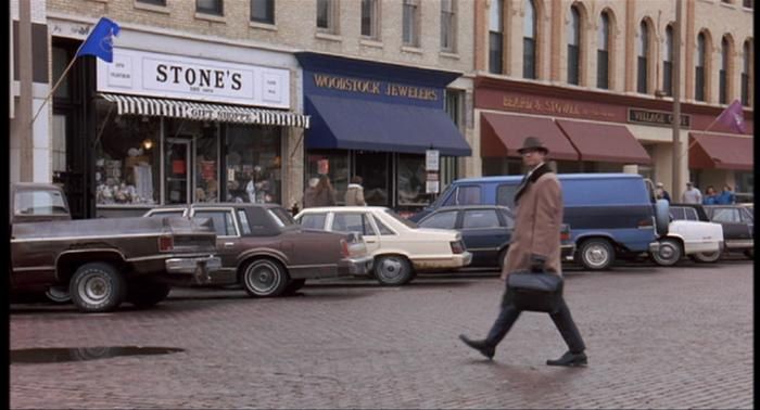
0     1     2     3     4     5     6     7     8     9
                  0     -   219   223   134   195   266   187   275   206   287
                  1   219     -   288   134   252   320   246   345   189   251
                  2   223   288     -   178   215   232   208   341   190   231
                  3   134   134   178     -   143   158   130   173   169   172
   Stage (1)      4   195   252   215   143     -   228   210   259   174   270
                  5   266   320   232   158   228     -   189   338   210   295
                  6   187   246   208   130   210   189     -   278   171   199
                  7   275   345   341   173   259   338   278     -   231   337
                  8   206   189   190   169   174   210   171   231     -   204
                  9   287   251   231   172   270   295   199   337   204     -

                        0     1     2     3     4     5     6     7     8     9
                  0     -     2     3     6     4    13     1     6     2     3
                  1     2     -     5     3     4    11    34     3     5     3
                  2     3     5     -    14     2     6    10    10     8     4
                  3     6     3    14     -     6     0     0     1    28     5
   Stage (2)      4     4     4     2     6     -     1     7     0     3    23
                  5    13    11     6     0     1     -     2     2     8     6
                  6     1    34    10     0     7     2     -     2     4     3
                  7     6     3    10     1     0     2     2     -     5    11
                  8     2     5     8    28     3     8     4     5     -     1
                  9     3     3     4     5    23     6     3    11     1     -

                        0     1     2     3     4     5     6     7     8     9
                  0     -     0     1     1     0     8     0     0     0     0
                  1     0     -     0     0     0     0    16     0     0     0
                  2     1     0     -     1     0     0     0     5     1     1
                  3     1     0     1     -     4     0     0     0    11     0
   Stage (3)      4     0     0     0     4     -     0     0     0     2    14
                  5     8     0     0     0     0     -     0     0     0     2
                  6     0    16     0     0     0     0     -     0     0     0
                  7     0     0     5     0     0     0     0     -     0     2
                  8     0     0     1    11     2     0     0     0     -     0
                  9     0     0     1     0    14     2     0     2     0     -

                        0     1     2     3     4     5     6     7     8     9
                  0     -     0     0     0     0   163     0     0     0     0
                  1     0     -     0     0     0     0   328     0     0     0
                  2     0     0     -     0     0     0     0   137     0     0
                  3     0     0     0     -     0     0     0     0    88     0
   Stage (4)      4     0     0     0     0     -     0     0     0     9   290
                  5   163     0     0     0     0     -     0     0     0     0
                  6     0   328     0     0     0     0     -     0     0     0
                  7     0     0   137     0     0     0     0     -     0     0
                  8     0     0     0    88     9     0     0     0     -     0
                  9     0     0     0     0   290     0     0     0     0     -

Table 2. Tables showing the number of matches found between the key frames of figure 6 at various stages
of the key frame matching algorithm of table 1. The image represents the table in each row with intensity
coding the number of matches (darker indicates more matches). Frames n and n + 5 correspond. The
diagonal entries are not included. Stage (1): matches from invariant indexing alone. Stage (2): matches
after neighbourhood consensus. Stage (3): matches after local correlation/registration verification. Stage
(4): matches after guided search and global verification by robustly computing epipolar geometry. Note
how the stripe corresponding to the correct entries becomes progressively clearer. The stages in this process
of frame matching can be compared to those in figure 9 for shot matching.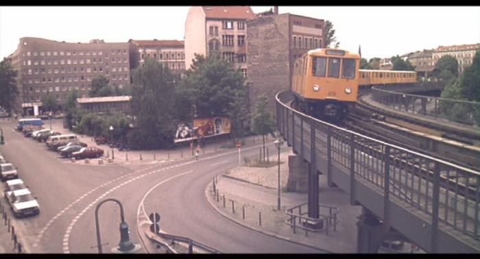
0                      1                     2                     3                     4

          5                      6                     7                     8                     9

Fig. 7. Verified feature matches after fitting epipolar geometry for the 10 key frames of figure 6. It is hard
to tell in these small images, but each feature is indicated by an ellipse and lines indicate the image motion
of the matched features between frames. In this case the matches are to the image below (top row) or
above(bottom row). Note that the spatial distribution of matched features indicates the extent to which the
images overlap.

three repeats of a basic sequence (with variations). Thus locations typically appear three times,
at least once in each sequence, and shots from two sequences are used here. Snapshots of the
progress at various stages of the algorithm are shown in figure 9. Statistics on the matching are
given in table 2.

3.1   Near neighbour indexing
By comparing the invariant vectors for each point over all frames, potential matches may be
hypothesized: i.e. a match is hypothesized if the invariant vectors of two points are within a
threshold distance. The basic query that the indexing structure must support is the “ε-search”,
i.e. “to find all points within distance ε of this given point”. We take ε to be 0.2 times the image
dynamic range (recall this is an image intensity SSD threshold).
     For the experiments in this paper we used a binary space partition tree, found to be more
time efficient than a k-d tree, despite the extra overhead. The high dimensionality of the invariant
space (and it is generally the case that performance increases with dimension) rules out many
indexing structures, such as R-trees, whose performances do not scale well with dimension.
     In practice, the invariant indexing produces many false putative matches. The fundamental
problem is that using only local image appearance is not sufficiently discriminating and each
feature can potentially match many other features. There is no way to resolve these mismatches
using local reasoning alone. However, before resorting to the non-local stages below, two steps
are taken. First, as a result of using several (three in this case) sizes of elliptical region for
each feature it is possible to only choose the most discriminating match. Indexing tables are
constructed for each size separately (so for example the largest elliptical neighbourhood can
only match that corresponding size), and if a particular feature matches another at more than
one region size then only the most discriminating (i.e. larger) is retained. Second, some features
are very common and some are rare. This is illustrated in figure 8 which shows the frequency
of the number of hits that individual features find in the indexing structure. Features that are
common are not very useful for matching because of the combinatorial cost of exploring all
the possibilities, so we want to exclude such features from inclusion in the indexing structure
(similar to a stop list in text retrival). Our method for identifying such features is to note that
a feature is ambiguous for a particular image if there are many similar-looking features in that
image. Thus intra-image indexing is first applied to each image separately, and features with five
or more intra-image matches are suppressed.
1 1 1
0.9 0.9 0.9
0.8 0.8 0.8
0.7 0.7 0.7
frequency
frequency
frequency
0.6 0.6 0.6
0.5 intra, s = 1.0 0.5 intra, s = 2.0 0.5 intra, s = 3.0
0.4 0.4 0.4
0.3 0.3 0.3
0.2 0.2 0.2
0.1 0.1 0.1
0 0 0
0 50 100 150 0 5 10 15 20 25 30 35 40 0 5 10 15 20 25 30
# hits # hits # hits
1 1 1
0.9 0.9 0.9
0.8 0.8 0.8
0.7 0.7 0.7
frequency
frequency
frequency
0.6 0.6 0.6
0.5 inter, s = 1.0 0.5 inter, s = 2.0 0.5 inter, s = 3.0
0.4 0.4 0.4
0.3 0.3 0.3
0.2 0.2 0.2
0.1 0.1 0.1
0 0 0
0 10 20 30 40 50 60 0 10 20 30 40 50 60 70 0 10 20 30 40 50 60
# hits # hits # hits
Fig. 8. Statistics on intra- and inter-image matching for the 15 images from the church at Valbonne (three
of which are shown in figure 1). For each scale (s = 1, 2, 3) the number of hits that each feature finds
in the index table is recorded. Distinctive features find 2-3 hits; features that find 20 or more hits are not
useful. The histograms show how the number of hits is distributed; note that as s increases, the maximum
number of intra-image hits drops. The number of inter-image hits (using only features deemed distinctive)
is fairly constant.
3.2 Filtering matches
Neighbourhood consensus: This stage measures the consistency of matches of spatially neigh-
bouring features as a means of verifying or refuting a particular match. For each putative match
between two images the K (= 10) spatially closest features are determined in each image giving,
for each matched feature, a set of image “neighbour” features. If at least N (= 1) neighbours
have been matched too, the original putative match is retained, otherwise it is discarded.
This scheme for suppressing putative matches that are not consistent with nearby matches
was originally used in [23, 29]. It is, of course, a heuristic but it is quite effective at removing
mismatches without discarding correct matches; this can be seen from table 2.
Local verification: Since two different patches may have similar invariant vectors, a “hit”
match does not mean that the image regions are affine related. For our purposes two pointsare deemed matched if there exists an affine geometric and photometric transformation which
registers the intensities of the elliptical neighbourhood within some tolerance. However, it is too
expensive, and unnecessary, to search exhaustively over affine transformations in order to verify
every match. Instead an estimate of the local affine transformation between the neighbourhoods
is computed from the linear filter responses. If after this approximate registration the intensity
at corresponding points in the neighbourhood differ by more than a threshold, or if the implied
affine intensity change between the patches is outside a certain range then the match can be
rejected. The thresholds used for the photometric transformation are that the offset must be at
most 0.5, and the scaling must be at most 2 (the images have dynamic range from 0 to 1).
Semi-local search for supporting evidence: In this step new matches are grown using a locally
verified match as a seed. The objective is to obtain other verified matches in the neighbourhood,
and then use these to grow still further matches etc. Given a verified match between two views,
the affine transformation between the corresponding regions is now known and provides infor-
mation about the local orientation of the scene near the match. The local affine transformation
can thus be used to guide the search for further matches which have been missed as hits, perhaps
due to feature localization errors, to be recovered and is crucial in increasing the number of cor-
respondences found to a sufficient level. This idea of growing matches was introduced in [19]
and also applied in [22].
Removing ambigous matches: While growing can produce useful matches that had been missed
it can also result in large numbers of spurious matches when there is repeated structure in a
region of an image. In effect, a feature corresponding to repeated structure can end up being
matched to several other features in the other frame. Such features are ambiguous and we give
each feature an “ambiguity score” which is the number of features it matches in the other frame.
Then we define the ambiguity of a (putative) match to be the product of the ambiguities for the
features. To reduce the effect of ambiguity, an “anti-ambiguity” filter is run over the matches at
this stage, greedily deleting the most ambiguous matching until no match has ambiguity score
greater than 6 (six).
3.3 Global constraints
Epipolar geometry: If the two frames are images of the same 3D location then the matches
will be consistent with an epipolar relation. It is computed here using the robust RANSAC
algorithm [6, 26, 29]. Matches which are inliers to the computed epipolar geometry are deemed
to be globally verified.
In some contexts (when the scene is flat or the camera centre has not moved between the two
frames) a homography relation might be more appropriate but the epipolar constraint is in any
case still valid.
Enforcing uniqueness: The epipolar geometry constraint does not enforce uniqueness of match-
ing but allows multi-matches, so long as they are all consistent with the epipolar geometry. As a
final step of the algorithm we completely suppress multi-matches by the same method as before
but this time only allowing an ambiguity of 1 (one).3.4 Evaluation and discussion
The number of matches at four stages of the algorithm is given in table 2. Matching using
invariant vectors alone (table 2, stage (1)), which would be equivalent to simply voting for the
key frame with the greatest number of similar features, is not sufficient. This is because, as
discussed above, the invariant features alone are not sufficiently discriminating, and there are
many mismatches, we return to this point in section 4. The neighbourhood consensus (table 2,
stage (2)), which is a semi-local constraint, gives a significant improvement, with the stripe of
correct matches now appearing. Local verification, (table 2, stage (3)), removes most of the
remaining mismatches, but the number of feature matches between the corresponding frames is
also reduced. Finally, growing matches and verifying on epipolar geometry, (table 2, stage (4)),
clearly identifies the corresponding frames. Figure 9 compares the progress of the four stages
for a matching and non-matching key-frame pair. Again it can be seen that most of the incorrect
matches have been removed by the neighbourhood consensus stage alone.
The matches between the key frames 4 and 9 (which are shown in detail in Figure 10) demon-
strate well the invariance to change of viewpoints. Standard small baseline algorithms fail on
such image pairs. Strictly speaking, we have not yet matched up corresponding frames because
we have not made a formal decision, e.g. by choosing a threshold on the number of matches
required before we declare that two shots match. In the example shown here, any threshold be-
tween 9 and 88 would do but in general a threshold on match number is perhaps too simplistic
for this type of task. As can be seen in figure 7 the reason why so few matches are found for
frames 2 and 7 is that there is only a small region of the images which do actually overlap. A
more sophisticated threshold would also consider this restriction.
Cost and time complexity: The cost of the various stages on a 2GHz Intel Xeon processor is as
follows: stage (1) takes 5+10 seconds (intra+inter image matching); stage (2) takes 0.4 seconds;
stage (3) takes less than one millisecond; stage (4) takes 15 + 4 seconds (growing+epipolar
geometry). In comparison feature detection takes a longer time by far (several minutes) than all
the matching stages. It is clearly linear in the number of frames.
The complexity of stage (1) intra-image matching is linear in the number of images and the
output is a set of features that find at most 5 hits within their own images. The complexity of
stage (1) inter-image matching is “data-dependent” (which is a nice way to say quadratic); the
cost of indexing depends on how the data is distributed in invariant space. A well-constructed
spatial indexing structure will have typical access time that is logarithmic in the number of fea-
tures. Generally, tight clusters cause problems because the number of neighbours to be recorded
increases quadratically with feature density. However, the intra-matching stage specifically ad-
dresses and reduces the problem of high density regions.
The complexity of stage (2) (neighbourhood consensus) is (using appropriate spatial index-
ing) K times the number of features detected per image, so can be considered to be linear in the
number of images. The complexity of stage (3) (intensity correlation and registration) is linear in
the number of putative matches to be verified so, because each feature is limited to at most five
putative matches, that process is also linear in the number of images. The algorithm variation of
performing correlation before neighbourhood consensus (i.e. stage (3) before stage (2)) makes
only a slight difference to the overall performance so we chose to bring in neighbourhood con-
sensus at the earliest possible stage to reduce cost. The complexity of growing is again linear in
the number of putative matches. Quite often, unrelated images have no matches between them2 7 2 6 Pairs Stage (1) invariant indexing Stage (2) neighbourhood consensus Stage (3) local verification Stage (4) growing epipolar uniqueness Fig. 9. Comparison of progress for matching (2 & 7) and non-matching (2 & 6) key frames. In both cases there are clearly many mis-matches at stage (1). These are almost entirely removed at stage (2). In the case of the matching pair (left) the correct matches remain, and there are many of these. In the case of the non-matching pair (right) only a few erroneous matches remain. Stage (3) removes more of the erroneous matches (right), though at a cost of removing some correct matches (left). The final stage (4) increases the number of matches (by growing), and epipolar geometry and uniqueness remove all erroneous matches for the pair on the right. The stages in this process are analogous to those in table 2 for matching single frames.
Fig. 10. Detail of matches for key frames 4 & 9. Note the large motion vectors resulting from the change
in camera elevation between shots – only one half of each image overlaps with the other.
after stages (2) and (3), and of course these do not have to be attended to so in practice the cost
seems to be incurred mostly by frames that do actually match. For example, for “Run Lola Run”
the number of epipolar geometries actually evaluated was about 18000, which is much smaller
than the worst case of about 5 million. So fitting epipolar geometry between all pairs of frames
is not really quadratic in the number of images and in practice pairs of frames with few putative
matches between are dispatched quickly.

               stage (1)              stage (2)             stage (3)              stage (4)

Fig. 11. Matching results using three keyframes per shot. The images represent the normalized 10 × 10
matching matrix for the test shots under the four stages of the matching scheme. See caption of table 2 for
details.

Using several key frames per shot: One way to address the problem of small image overlap
is to aggregate the information present in each shot before trying to match. As an example, we
chose three frames (30 frames apart) from each of the ten shots and ran the two-view matching
algorithm on the resulting set of 3 × 10 = 30 frames. In the matrix containing number of
matches found, one would then expect to see a distinct 3 × 3 block structure. Firstly, along the
diagonal, the blocks represent the matches that can be found between nearby frames in each
shot. Secondly, off the diagonal, the blocks represent the matches that can be found between
frames from different shots. We coarsen the block matrix by summing the entries in each 3 × 3
block and arrive at a new 10 × 10 matrix Mij ; the diagonal entries now reflect how easy it
is to match within each shot and the off-diagonal entries how easy it is to match across shots.
Thus, the diagonal entries can be used to normalize the other entries in the matrix by forming a
new matrix with entries given by Mii Mij Mjj         (and zeroing its diagonal). Figure 11 shows
                                    −1/2        −1/2

these normalized matrices as intensity images, for the various stages of matching.
    Note that although one would expect the entries within each 3 × 3 block between matching
shots to be large, they can sometimes be zero if there is no spatial overlap (e.g. in a tracking
shot). However, so long as the three frames chosen for each shot cover most of the shot, there is
a strong chance that some pair of frames will be matched. Consequently, using more than one
key-frame per shot extends the range over which the wide baseline matching can be leveraged.
The algorithm for key-frame matching is summarized in table 1. However, the use of more and
more key frames per shot is clearly not scalable for matching the entire movie. This is one of
the motivations for moving to shot based matching descibed in the following section.
4 Matching between shots using tracked features
In this section we describe how the ideas of wide baseline matching of the previous section can
be developed into an algorithm for shot matching. Again, our measure of success is that we
match shots which include the same location but not shots of different 3D locations.
We will employ the temporal information available within a shot from contiguous frames.
Frame-to-frame feature tracking is a mature technology and there is a wealth of information that
can be obtained from putting entire feature tracks (instead of isolated features) into the indexing
structure. For example, the measurement uncertainty, or the temporal stability, of a feature can
be estimated and these measures used to guide the expenditure of computational effort; also, 3D
structure can be used for indexing and verification. In this way the shot-with-tracks becomes the
basic video matching unit, rather than the frames-with-features.
Our aim is to find analogues of the processes on which the successful key-frame matching
algorithm of section 3 were built. For example an analogue to a feature in a frame, an analogue of
neighbourhood consensus, but now with the entire set of frames of the shot available for our use.
As before we first describe the features that will be used in the indexing structure (section 4.1),
and then the stages in using these features to establish sub-sets of matching shots (section 4.2).
The method is evaluated using all the shots of the film ’Run Lola Run’, with a total of 1111 shot
and on the film ’Groundhog Day’, with a total of 753 shots.
4.1 Invariant descriptors for tracks
The overall aim here is to extract stable and distinctive descriptors over the entire shot. Track
persistence will be used to measure stability – so that a feature which is only detected in one
frame, for example, will not be included. In this way weak features which only appear momen-
tarily, i.e. are unstable, are discarded.
The feature extraction and description proceeds as follows. First, feature detection is per-
formed independently in each frame (using affine interest points and MSE regions, in the same
manner as described in section 2). Second, within each shot short baseline feature tracking is
performed using an adaptive disparity threshold with a correlation tracker, followed by removal
of ambiguous matches and robust fitting of between-frame epipolar geometry. (Here, “adaptive”
means that an initial disparity of 10 pixels is used and if the number of final between-frame
matches so obtained is less than 100 then the process is retried with a disparity threshold of 20
pixels). The output of this stage is a set of feature tracks for each shot. Third, each feature track
lasting for 20 or more frames is broken into contiguous fragments each of which is 20 to 30
frames long. Given a fragment, the invariants from section 2 are computed for each frame of the
fragment and the resulting descriptors registered and aggregated by averaging. The aggregated
filter response becomes the descriptor of that fragment.
The motivation for splitting the track into fragments is twofold, one theoretical and one
practical. The theoretical reason is an attempt to avoid averaging together features that could
have “drifted” in appearance from the start of the track to the end. This is possible because
the correlation tracker only compares the appearance of features in consecutive frames. The
practical reason is to make the aggregation of invariants feasible: if no track is longer than 30
frames then it is not necessary to hold more than 60 frames in memory at any one time. The
threshold of 20 frames (i.e. about a second) means that any shot shorter than this is not currently
matched. Also tracks that are broken are not included, for example a background track that iscut by foreground object which temporarily occludes it, or a track that has a feature drop-out
for a single frame. Nevertheless, there are generally sufficient supra-threshold tracks as shown
in figure 15, and the threshold has the desired effect of suppressing many short unstable tracks.
The number 20 is of course a parameter which could be varied; see the results section 4.3 and
figure 18 in particular.
4.2 Shot matching
The process of matching shots using tracks as descriptors proceeds analogously to that of match-
ing images using features as descriptors. In the wider sense of the word “feature”, tracked image
features are the features that we extract from each shot. However, there are several complications
that appear due to the extra temporal dimension.
Near neighbour indexing: The invariant indexing uses as its basic unit track fragments but
since we are ultimately interested in matching complete tracks, there are book-keeping over-
heads that did not arise in the case of single frames.
An important point is that some invariant descriptors (for fragments) are very common and
some are rare. Descriptors that are common are not very useful because they cause confusion
in the matching, so we want to exclude such features from inclusion in the indexing structure,
and concentrate on more distinctive features. We identify indistinctive features by noting that a
feature is ambiguous for a particular shot if there are many similar-looking features in that shot.
Thus intra-shot indexing is first applied to each shot separately, and features with six or more
intra-shots matches are suppressed. This procedure is a generalization of the distinctiveness
approach employed in key frame matching.
Two fragments are deemed matched if in addition to having similar invariants they also
overlap temporally. This is clearly necessary since the two fragments may come from the same
track but also addresses the observation that, in a single shot, the same scene element may
be observed many times without our being able to track it continously (e.g. due to temporary
occlusions): so long as tracks do not overlap temporally they do not detract from each other’s
distinctiveness. In inter-shot matching, each putatively matching pair of fragments coming from
different shots (and therefore different tracks) should vote only once for their tracks.
The opposite alternative, allowing the fragments from each track to vote independently
would unfairly favour long tracks over short ones; this could be addressed by using weighted
voting (the weight that a track fragment’s vote has would be proportional to the inverse, or
maybe the inverse square, of the length of the track) but we did not experiment with this.
Filtering matches using photometric and geometric constraints: The neighbourhood
consensus stage differs in two ways from the single frame implementation. Firstly the notion of
distance between two tracks must be elucidated: we took it to be the minimum image distance
over all frames that the tracks shared. Secondly, in order for two tracks to be neighbours they
must be temporally overlapping. Otherwise this stage is as for single frames.
In general, given two putatively matched tracks (from different shots) there is a lot of infor-
mation that can be used to verify the match since each frame containing the first track could in
principle be compared to each frame containing the second track. For example, when doing a
correlation test for tracks of length l1 and l2 , there are l1 ×l2 pairs of frames across which the cor-
relation could be carried out and there are correspondingly many more correlation coefficients
to consider when making a decision. It is expensive to do this so we limited ourselves to every10th frames; the final between-shot score was taken to be the median of all the between-frame
scores.
In the growing stage, given two putatively matched tracks, we consider their (temporal)
midpoints and carry out single-frame growing there (in practice we round the midpoint frame
numbers to their nearest multiple of 10 since this reduces the number of frames that must be
kept in memory by an order of magnitude). Finally, ambiguous matches are removed in the
same manner as for frame matching.
Global constraints: Epipolar geometry is another constraint that is defined between a pair
of frames. To use it for tracks matched across two shots we choose first a pair of frames that
has the largest number of matches between them, and apply a between-frame epipolar geometry
constraint there. Unfortunately, there may be pairs of tracks that are not tested by this because
at least one of them is temporally disjoint from the pair of frames used for testing So we choose
a new pair of frames so as to maximize the number of untested tracks that would be included
in a test carried out between those frames. This is repeated until all putatively matched tracks
have been tested. To make a final decision, we form for each pair of tracks the ratio between the
number of tests it passed and the number of tests it took part in. Any pair of tracks with ratio
below 0.5 is rejected.
After epipolar geometry and uniqueness checking we look more closely at the pairwise shot
matches that remain. Any pair of shots with more than 100 matches between them is deemed
matched. Pairs with fewer matches than this are subjected to a (slightly expensive) full two-
view matching procedure to see if the number of matches can be increased. If a pair of features
between the chosen frames match then we declare that [any] tracks containing those features
also match. The pair of frames is chosen to give the maximal number of matched tracks between
them.
Finally, we threshold at 10 matches. The mopping up stage does not have an analogue for
frame matching. The entire algorithm is summarized in table 4.
4.3 Results of shot matching
We carry out three sets of tests on ’Run Lola Run’. In the first we compare the shot matching
performance on the same 10 shots used in section 3. In the second we increase the number of
shots to 55. This is still a manageable number, so that performance can be compared to ground
truth. Finally, we increase the number of shots to 1111, which is the entire movie.
10 test shots: A typical tracking performance is illustrated in figures 12-13, and matches be-
tween two of the test shots are illustrated in figure 14. The number of track matches for various
stages of the shot matching algorithm are given in table 3. As in the case of the key-frame match-
ing algorithm the results are correct (no false positives and no false negatives), and there are a
healthy number of tracks matched between all shots of the same location.
55 shots: As a stepping stone between processing 10 shots and 1000 we ran the algorithm on
a subset of 55 shots for which we manually obtained ground truth. A few shots are used from
the introductory sequence and then about 15 shots are used from each of the three repeating
sequences in the film. The results are shown in three figures.
Figure 17 gives the results of running exactly the same algorithm as in the 10-shot example
above. Figure 18 gives the results for a lower minimum length of tracks (and track fragments),Fig. 12. Tracking performance. Four frames from a single shot from the movie (this shot corresponds to shot 7 in figure 6). Each white curve shows a feature track. A detail is shown in figure 13. There were 68521 tracks in this shot, of which 60% had length 2 or 3. Only (3.7%) of tracks were 20 or more frames long, however this is 2553 tracks which is plenty for matching. The track length distribution is shown in figure 15. Fig. 13. Detail from figure 12, showing the motion of one fairly large feature across its 30-frame trajectory. Fig. 14. Matched tracks. The upper row shows tracks for shot 2, the lower row matches for shot 7 of figure 6. Tracks shown in blue have been matched to some other track in the other shot. Tracks shown in green have been matched to a track that is visible in the corresponding frame in the other shot. Near the end of the row motion blur defeats the feature detectors and large image motion defeats the tracking strategy. In shot 2 there were 41606 tracks in total, 1734 (4.2%) of which were 20 frames or more long. The histogram of these track lengths is shown in figure 15.
250                                                  140

                                                        120
   200
                                                        100

   150
                                                         80

   100                                                   60

                                                         40
    50
                                                         20

     0                                                    0
     10    20   30    40   50    60    70   80    90       0      20     40     60      80     100    120

    Fig. 15. Histogram of track lengths 20 or more frames long, for the two shots shown in figure 14.

Fig. 16. Match densities. For the first three matched pairs of shots from the 10-shot data shown in figures 6
these plots record the number of between-frame feature matches as a function of frame numbers. The areas
of blue represent pairs of frames between which there were few matches and red areas represent high
numbers of matches. Note that in the first two cases the plots indicate how to register the two sequences
temporally. The last plot has a gap in the middle due to tracking failure. Of course, in general a pair of
shots might not have a temporal registration, say if the camera motion is very different in the two shots.
0 1 2 3 4 5 6 7 8 9
0 - 15 16 7 0 756 3 57 8 24
1 15 - 12 17 0 16 1024 63 14 15
2 16 12 - 2 0 17 5 490 9 14
3 7 17 2 - 0 10 10 17 85 18
Stage (1) 4 0 0 0 0 - 0 1 0 0 53
5 756 16 17 10 0 - 7 51 13 28
6 3 1024 5 10 1 7 - 14 4 15
7 57 63 490 17 0 51 14 - 40 64
8 8 14 9 85 0 13 4 40 - 8
9 24 15 14 18 53 28 15 64 8 -
0 1 2 3 4 5 6 7 8 9
0 - 1 0 0 0 730 0 18 0 4
1 1 - 0 3 0 1 995 9 1 0
2 0 0 - 0 0 1 0 468 4 7
3 0 3 0 - 0 0 2 2 72 10
Stage (2) 4 0 0 0 0 - 0 0 0 0 52
5 730 1 1 0 0 - 0 19 0 5
6 0 995 0 2 0 0 - 0 0 4
7 18 9 468 2 0 19 0 - 6 30
8 0 1 4 72 0 0 0 6 - 2
9 4 0 7 10 52 5 4 30 2 -
0 1 2 3 4 5 6 7 8 9
0 - 0 0 0 0 381 0 0 0 0
1 0 - 0 0 0 0 367 0 0 0
2 0 0 - 0 0 0 0 259 0 0
3 0 0 0 - 0 0 0 0 35 0
Stage (3) 4 0 0 0 0 - 0 0 0 0 25
5 381 0 0 0 0 - 0 0 0 0
6 0 367 0 0 0 0 - 0 0 0
7 0 0 259 0 0 0 0 - 0 0
8 0 0 0 35 0 0 0 0 - 0
9 0 0 0 0 25 0 0 0 0 -
0 1 2 3 4 5 6 7 8 9
0 - 0 0 0 0 381 0 0 0 0
1 0 - 0 0 0 0 367 0 0 0
2 0 0 - 0 0 0 0 259 0 0
3 0 0 0 - 0 0 0 0 86 0
Stage (4) 4 0 0 0 0 - 0 0 0 0 162
5 381 0 0 0 0 - 0 0 0 0
6 0 367 0 0 0 0 - 0 0 0
7 0 0 259 0 0 0 0 - 0 0
8 0 0 0 86 0 0 0 0 - 0
9 0 0 0 0 162 0 0 0 0 -
Table 3. Tables showing the number of track matches found between the shots illustrated by the key-frames
of figure 6 at various stages of the shot matching algorithm II. Compare with table 2 where details of shot
matching using key frames are given in the caption. Note how much better the results are for invariant
indexing with tracks in shots compared with features in single images.10 instead of 20. It can be seen that this lower length value increase the number of matches
found as there are more dark areas in the imges. This suggests that the limit of 20 frames rejects
useful matches and so is too high.
The structure of the film is clearly reflected in these images: first there is the introduction
sequence (left columns and top rows of matrix) and then follow three sequences that approx-
imately repeat; the sloping structures are sequences of shots that match across different parts
of the movie. Thus, the first “meta-row” of the matrix shows that the first of the three repeat-
ing sequences matched the last two sequences and the second row shows the second sequence
matched the first and last (the matrix is symmetric, of course).
Comparing with ground truth (figure 19) one gets a fair agreement in overall structure but
some things are of course more weakly matched (lighter shades of grey in the images) than the
binary image showing the ground truth matches.
Fig. 17. Progress of matching over 55 shots with tracks of length 20 or more. There are about 15 shots
taken from each of the three repeating sequences and the sloping structures that can be seen reflect the
repetition of these matching sequences of shots. The intensity indicates the number of matches.
Fig. 18. Progress of matching over 55 shots with tracks of length 10 or more. This is just a parameter
variation of figure 17.
1111 shots: Finally, in figure 20 we show the match matrix for all 1111 shots detected in “Run
Lola Run”. The same structure as before is visible but at higher resolution. Unfortunately, this
makes it difficult to see individual shots (which would be one pixel across) so to bring out
the structure the raw images have been processed by dilating with a box filter of width 7 and(a) (b) (c) Fig. 19. (a) Ground truth for matching over 55 shots. Compare with the computed match matrices in fig- ures 17 and 18. Unlike those figures, which use intensity to indicate the strength of the shot matches, this one is a binary image. (b) binarized version of the match matrix from figure 17. (c) binarized version of the match matrix from figure 18. In (b) and (c) the number of matches was first thresheld at 10 and then the “transitive closure” of the resulting binary relation was computed. clamping the intensities to the range 0-255. Examples of particular shot matches can be seen in figures 21 through 25. Fig. 20. Progress of matching over 1111 shots. The raw counts of matches have been processed with a morphological dilation for ease of viewing. Comparison of two methods: Is it better, then, to use frame-to-frame matching on key frames than shot-to-shot matching? The question is not easy to answer empirically on the scale of a full film because it is intractable to run a two-view match on a every pair of key-frames from a whole movie. The frame-to-frame matching software that we used is certainly better developed and tuned than the shot matching software so one might expect key-frames to work better but not for any interesting reason. Theoretically the wastefulness of using key-frame matching on an entire movie is a big impediment; another theoretical reason for avoiding key-frames is that it is hard to know how many frames to include to get good representation of each shot (especially when the camera pans). On the other hand, feature tracks get the full benefit of temporal stability and will certainly summarize entire shots (as far as it is possible to do using the features detected in each frame).
You can also read