MASS: MULTI-ATTENTIONAL SEMANTIC SEGMENTATION OF LIDAR DATA FOR DENSE TOP-VIEW UNDERSTANDING
←
→
Page content transcription
If your browser does not render page correctly, please read the page content below
1
MASS: Multi-Attentional Semantic Segmentation of
LiDAR Data for Dense Top-View Understanding
Kunyu Peng1 , Juncong Fei2,3 , Kailun Yang1 , Alina Roitberg1 , Jiaming Zhang1 , Frank Bieder2 ,
Philipp Heidenreich3 , Christoph Stiller2 , and Rainer Stiefelhagen1
Abstract—At the heart of all automated driving systems is
the ability to sense the surroundings, e.g., through semantic
segmentation of LiDAR sequences, which experienced a re-
markable progress due to the release of large datasets such
arXiv:2107.00346v1 [cs.CV] 1 Jul 2021
as SemanticKITTI and nuScenes-LidarSeg. While most previous
works focus on sparse segmentation of the LiDAR input, dense
output masks provide self-driving cars with almost complete
environment information. In this paper, we introduce MASS -
a Multi-Attentional Semantic Segmentation model specifically
built for dense top-view understanding of the driving scenes. Our
framework operates on pillar- and occupancy features and com-
prises three attention-based building blocks: (1) a keypoint-driven
graph attention, (2) an LSTM-based attention computed from a
vector embedding of the spatial input, and (3) a pillar-based
attention, resulting in a dense 360◦ segmentation mask. With
extensive experiments on both, SemanticKITTI and nuScenes-
LidarSeg, we quantitatively demonstrate the effectiveness of
our model, outperforming the state of the art by 19.0% on
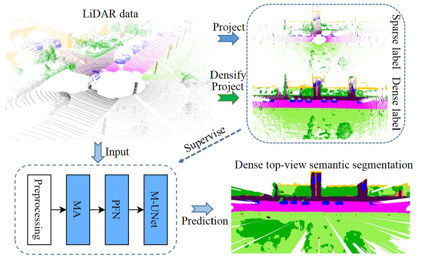
Fig. 1: An overview of dense top-view semantic segmentation
SemanticKITTI and reaching 32.7% in mIoU on nuScenes- based on the proposed MASS framework, where LiDAR data
LidarSeg, where MASS is the first work addressing the dense is half painted by its semantic label. In the model structure,
segmentation task. Furthermore, our multi-attention model is MA denotes our multi-attention mechanism, PFN denotes the
shown to be very effective for 3D object detection validated on pillar feature net, and M-UNet denotes the modified UNet. The
the KITTI-3D dataset, showcasing its high generalizability to
other tasks related to 3D vision.
network is supervised by the labeled grid cell and evaluated
by the visible region shown by the occupancy map.
Index Terms—Semantic segmentation, attention mechanism,
LiDAR data, automated driving, intelligent vehicles.
segmentation employing 2D Convolutional Neural Networks
I. I NTRODUCTION (CNNs) has evolved to a well developed field, where FCN [4],
reliable semantic understanding of the surroundings is DeepLab [5], and ERFNet [6], [7] represent prominent archi-
A crucial for automated driving. To this end, multi-modal
input captured, e.g., by cameras, LiDARs, and radars is
tectures. Recent emergence of large-scale datasets for semantic
segmentation of 3D data, such as SemanticKITTI [8] and
frequently leveraged in automated vehicles [1], [2], [3]. Se- nuScenes-LidarSeg [9] has allowed the community to go be-
mantic segmentation is one of the most essential tasks in yond the conventional 2D semantic segmentation and develop
automated driving systems since it predicts pixel- or point- novel methods operating on 3D LiDAR point clouds [10].
level labels for the surrounding environment according to 3D point cloud data generated through LiDAR sensors has
different input modalities. Over the past few years, semantic multiple advantages over 2D data [11]. Such point cloud
data complements traditional 2D image projection techniques
This work was funded by the German Federal Ministry for Economic and has direct access to the depth information, leading to a
Affairs and Energy within the project “Methoden und Maßnahmen zur Ab-
sicherung von KI basierten Wahrnehmungsfunktionen für das automatisierte
richer spatial information about the surrounding environment.
Fahren (KI-Absicherung)”. This work was also supported in part through the Furthermore, 3D LiDAR point clouds directly incorporate
AccessibleMaps project by the Federal Ministry of Labor and Social Affairs distance and direction information, while camera-based sys-
(BMAS) under the Grant No. 01KM151112, in part by the University of
Excellence through the “KIT Future Fields” project, and in part by Hangzhou
tems can only infer through generated images to reconstruct
SurImage Company Ltd. The authors would like to thank the consortium for distance- and orientation-related information. Of course, Li-
the successful cooperation. (Corresponding author: Juncong Fei.) DAR data also brings certain challenges. Since 3D point cloud
1 Authors are with Institute for Anthropomatics and Robotics, Karl-
data is sparse, unordered, and irregular in terms of its spatial
sruhe Institute of Technology, Germany (e-mail: {kunyu.peng, kailun.yang,
alina.roitberg, jiaming.zhang, rainer.stiefelhagen}@kit.edu). shape, it is not straightforward to transfer mature 2D CNN-
2 Authors are with Institute for Measurement and Control Systems, Karl-
based approaches to LiDAR data. To solve this problem, Point-
sruhe Institute of Technology, Germany (e-mail: juncong.fei@partner.kit.edu, Net [12] extracts point-level features, whereas PointPillars [13]
frank.bieder@kit.edu, stiller@kit.edu).
3 Authors are with Stellantis, Opel Automobile GmbH, Germany. forms a top-view pseudo image based on high-dimensional
Code will be made publicly available at github.com/KPeng9510/MASS pillar-level features in order to utilize a 2D backbone for 3D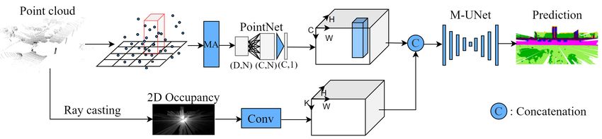
2

object detection. The pillar feature net is also leveraged in                          II. R ELATED W ORKS
our PillarSegNet architecture, which is put forward as the        A. Image Semantic Segmentation and Attention Mechanism
backbone in our framework. Some works focus on predicting
                                                                      Dense pixel-wise semantic segmentation has been largely
point-level semantic class for each LiDAR point given a 3D
                                                                  driven by the development of natural datasets [21], [22] and ar-
point cloud such as the approaches proposed by [14], [15],
                                                                  chitectural advances since the pioneering Fully Convolutional
[16], [17], which realize sparse segmentation. In contrast to
                                                                  Networks (FCNs) [4] and early encoder-decoder models [23],
these approaches, our PillarSegNet generates dense top-view
                                                                  [24]. Extensive efforts have been made to enrich and enlarge
semantic segmentation given a sparse 3D point cloud as the
                                                                  receptive fields with context aggregation sub-module designs
input, which can even accurately yield predictions on those
                                                                  like dilated convolutions [25] and pyramid pooling [5], [26].
locations without any LiDAR measurements (see Fig. 1). This
                                                                  In the Intelligent Transportation Systems (ITS) field, real-
dense interpretation is clearly beneficial to essential upper-
                                                                  time segmentation architectures [6], [27] and surrounding-
level operating functions such as the top view based navigation
                                                                  view perception platforms [28], [29], [30] are constructed for
for automated driving [18].
                                                                  efficient and complete semantic scene understanding.
   In this paper, we introduce a Multi-Attentional Semantic           Another cluster of works takes advantage of the recent
Segmentation (MASS) framework, which aggregates local-            self-attention mechanism in transformers [31] to harvest long-
and global features, and thereby boosts the performance of        range contextual information by adaptively weighing features
dense top-view semantic segmentation. MASS is composed            either in the temporal [31] or in the spatial [27], [32] domain.
of Multi-Attention (MA) mechanisms, a pillar feature net          With focus set on scene segmentation, DANet [32] integrates
(PFN), and a modified UNet (M-UNet) utilized for dense top-       channel- and position attention modules to model associations
view semantic segmentation, as depicted in Fig. 1. Our MA         between any pair of channels or pixels. In ViT [33] and
mechanisms comprise three attention-based building blocks:        SETR [34], transformer is directly applied to sequences of
(1) a keypoint-driven graph attention, (2) an LSTM-based          image patches for recognition and segmentation tasks. In
attention computed from a vector embedding of the spatial         Attention Guided LSTM [35], a visual attention model is
input, and (3) a pillar-based attention. The proposed MASS        used to dynamically pool the convolutional features to capture
model is first evaluated on the SemanticKITTI dataset [8]         the most important locations, both spatially and temporally.
to verify its performance compared with the state-of-the-art      In Graph Attention Convolution [36], the kernels are carved
surround-view prediction work [19] and then validated on the      into specific shapes for structured feature learning, selectively
nuScenes-LidarSeg dataset [9], where our framework is the         focusing on the relevant neighboring nodes. FeaStNet [37],
first addressing the dense semantic segmentation task. Finally,   sharing a similar spirit, learns to establish correlations between
we validate the effectiveness of PointPillars enhancement with    filter weights and graph neighborhoods with arbitrary con-
our MA mechanism in terms of cross-task generalization.           nectivity. Concurrent attention design has also been exploited
  This work is an extension of our conference paper [20],         to learn more discriminative features [27], [32], [38]. For
which has been extended with the novel MA mechanism               example, TANet [38] collectively considers channel-, point-,
design, a detailed description of the proposed PillarSegNet       and voxel-wise attention by stacking them to aggregate multi-
backbone model, along with an extended set of experiments         level highlighted features.
on multiple datasets. In summary, the main contributions are:         While self-attention mechanism has been widely applied
                                                                  in image-based scene parsing, it is underresearched in the
                                                                  field of semantic segmentation of LiDAR input. We leverage
  •   We introduce MASS, a Multi-Attentional Semantic Seg-
                                                                  such attention operations to better aggregate features from
      mentation framework for dense top-view surrounding un-
                                                                  different points of view and propose a generic multi-attentional
      derstanding. We present an end-to-end method PillarSeg-
                                                                  framework for dense semantic segmentation with improved
      Net to approach dense semantic grid map estimation as
                                                                  discriminative representations.
      the backbone of our MASS framework, by using only
      sparse single-sweep LiDAR data.
  •   We propose Multi-Attention (MA) mechanisms com-             B. LiDAR Point Cloud Semantic Segmentation
      posed of two novel attentions and pillar attention to          Unlike image-based scene parsing, the interest in LiDAR
      better aggregate features from different perspectives and   point cloud semantic segmentation has been rapidly blos-
      to boost the performance of dense top-view semantic         soming until very recently with the appearance of large-
      segmentation given 3D point cloud input.                    scale datasets [8], [9], [39], [40], which provide rich data
  •   Experiments and qualitative comparisons are conducted       for supervised training and open up the application in 360◦
      firstly on SemanticKITTI [8], nuScenes-LidarSeg [9], and    point-wise surrounding understanding. Since the introduction
      then on the KITTI-3D dataset [21], to verify the effec-     of PointNet [12], many learning-based methods have emerged.
      tiveness of MA separately for dense top-view semantic       The SqueezeSeg family [41], [42] projects the 3D point
      segmentation and 3D object detection.                       cloud into 2D pseudo images for processing, and plenty
  •   A comprehensive analysis is presented on dense top-view     of subsequent methods follow this trend by mapping the
      semantic surrounding understanding with different atten-    3D LiDAR data under a forward-facing view or a bird’s
      tion setups individually on SemanticKITTI, nuScenes-        eye view, and thereby inherit the advancements in image
      LidarSeg, and KITTI-3D datasets.                            semantic segmentation using 2D fully convolutional networks.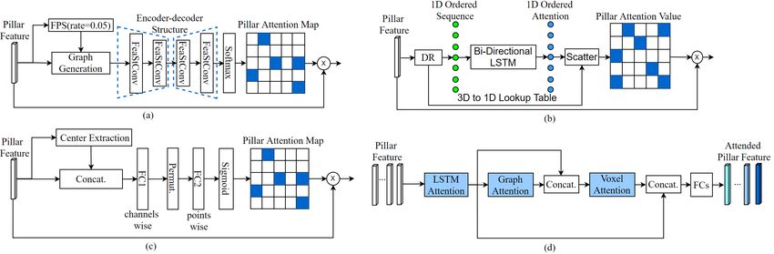
3

Fig. 2: Overview of the proposed MASS framework. Given a 3D point cloud obtained from LiDAR, MASS first executes
pillar-level feature encoding and computes optional 2D occupancy features in two parallel streams. The point cloud is first
rasterized into several pillars and MA generates attention values for these pillars. The attended pillar-level features are extracted
through the PointNet [12] architecture, whereas the observability features are encoded from a 2D occupancy map generated
through ray casting. Both features will be combined through the concatenation operation. Then, we leverage a modified UNet
to predict a dense top-view semantic grid map from the aggregated features. The final depicted prediction result is filtered by
the 2D occupancy map to exclude the occluded areas.

RangeNet++ [14] exploits a transformation to obtain spherical       semantic surrounding understanding [1], [29], [58].
images and employs 2D convolutions for semantic segmenta-
tion. The SalsaNet family [43], [44] presents fast architectures,              III. MASS: P ROPOSED F RAMEWORK
which have been validated either in the top-down bird’s eye
view [43] or in the spherical range view (i.e., panoramic              In this section, we introduce MASS - a new framework for
view) [44]. Triess et al. [15] leverage a scan unfolding and a      Multi-Attentional Semantic Segmentation given LiDAR point
cyclic padding mechanism to recover the context information         cloud data as input. First, we put forward a backbone model
at the horizontal panorama borders, which helps to eliminate        for dense top-view semantic segmentation given single sweep
point occlusions during the spherical projection in [14]. Such      LiDAR data as input. Then, we utilize Multi-Attention (MA)
unfolding and ring padding are similar to those in panoramic        mechanisms to aggregate local- and global features, and guide
scene parsing [45], and thus we consider that this line of          the network to specifically focus on feature map regions which
research can benefit from the latest progress in omnidirectional    are decisive for our task.
image segmentation like attention mechanisms [27].                     Conceptually, MASS comprises two building blocks: Pil-
                                                                    larSegNet – a novel dense top-view semantic segmentation ar-
   Instead of using range images, some methods utilize a
                                                                    chitecture, which extracts pillar-level features in an end-to-end
grid-based representation to perform top-view semantic seg-
                                                                    fashion, and an MA mechanism, with an overview provided
mentation [19], [46], [47], [48], [49]. GndNet [49] uses
                                                                    in Fig. 2. The proposed MA mechanism itself covers three
PointNet [12] to extract point-wise features and semantically
                                                                    attention-based techniques: a key-node based graph attention,
segment ground sparse data. PolarNet [50] quantizes the points
                                                                    an LSTM attention with dimensionality reduction of the spatial
into grids using their polar bird’s eye view coordinates. In
                                                                    embedding, and a pillar attention derived from the voxel
a recent work, Bieder et al. [19] transform 3D LiDAR data
                                                                    attention in TANet [38]. In the following, key principles of
into a multi-layer grid map representation to enable an effi-
                                                                    PillarSegNet and the proposed MA mechanisms are detailed.
cient dense top-view semantic segmentation of LiDAR data.
However, it comes with information loss when generating
the grid maps and thus performs unsatisfactorily on small-          A. PillarSegNet Model
scale objects. To address these issues, we put forward a novel         A central component of our framework is PillarSegNet –
end-to-end method termed PillarSegNet, which directly learns        a novel model for dense top-view semantic segmentation of
features from the point cloud and thereby mitigates the po-         sparse single LiDAR sweep input. In contrast to the previously
tential information loss. PillarSegNet divides the single-sweep     proposed grid-map based method [19], PillarSegNet directly
LiDAR point cloud into a set of pillars, and generates a dense      constructs pillar-level features in an end-to-end fashion and
semantic grid map using such sparse LiDAR data. Further,            then predicts dense top-view semantic segmentation. In ad-
the proposed MASS framework intertwines PillarSegNet and            dition to the pillar-level feature, occupancy feature is also
multiple attention mechanisms to boost the performance.             utilized in the PillarSegNet model as aforementioned to ag-
   There are additional methods that directly operate on 3D         gregate additional free-space information generated through
LiDAR data to infer per-point semantics using 3D learning           an optional feature branch, which is verified to be critical for
schemes [51], [52], [53] and various point cloud segmentation-      improving dense top-view semantic segmentation performance
based ITS applications [54], [55], [56], [57]. Moreover, LiDAR      compared with the model only utilizing pillar feature.
data segmentation is promising to be fused with image-based            PillarSegNet comprises a pillar feature net derived from
panoramic scene parsing towards a complete geometric and            PointPillars [13], an optional occupancy feature encoding
4 branch, a modified UNet architecture as the 2D backbone, and a dense semantic segmentation head realized by a logits layer. In later sections, the extensive experiments will verify that leveraging pillar feature net from [13] generates better repre- sentation than the grid-map-based state-of-the-art method [19]. Pillar Feature Encoding. Since 3D point cloud does not have regular shapes compared with 2D images, mature 2D CNN-based approaches cannot directly aggregate point cloud features. In order to utilize well-established approaches based on 2D convolutions, we first rasterize the 3D point cloud into Fig. 3: A generation procedure comparison between visibility a set of pillars on the top view, then pillar-level feature is feature (left) and observability feature (right). extracted through the pillar feature net and, finally, a pseudo image is formed on the top view. In the following, C marks the dimensionality of the point a slightly modified version based on the aforementioned encoding before being fed into the pillar feature net, P denotes visibility feature. The occupancy feature utilized in MASS is the maximum number of pillars, and the maximum number of called as observability feature encoded in the dense 2D top- augmented LiDAR points inside a pillar is N . We note that view form. The observability is slightly different compared only non-empty pillars are considered. If the generated pillars with the aforementioned visibility. First, it leverages pillars to or the augmented LiDAR points have not reached the afore- take the place of the voxel representation. Second, the three mentioned maximum numbers, zero padding is leveraged to states in visibility feature are discarded and the accumulated generate a fixed-size pseudo image. If the numbers are higher ray passing number is used to encode occupancy on the top than the desired numbers, random sampling is employed to view. Finally, a densely encoded occupancy feature map on assure the needed dimensionality. Consequently, the size of the top view is obtained. the tensor passed to PointNet in the next step is therefore (P, N, C). The point feature is encoded through PointNet [12] com- B. Key-node based Graph Attention posed of fully connected layers sharing weights among points Since 3D point cloud is relatively noisy [60], only few together with BatchNorm and ReLU layers to extract a high- points contain significant clues for dense top-view semantic level representation. segmentation. Thereby, we propose a novel key-node based Then, pillar-level feature is generated through the max graph attention mechanism which propagates relevant cues operation among all the points inside a pillar and the tensor from key-nodes to the other nodes. The representative node representation is changed to (P, C). Finally, these pillars are for each pillar is generated through a max operation among scattered back according to their coordinates on the xy plane to all points inside a non-empty pillar. Farthest Point Selection generate a top-view pseudo image for the input of the modified (FPS) is leveraged to generate the key-node set in a high- UNet backbone for semantic segmentation. level representation whose information is used to enrich the Occupancy Feature. Occupancy feature encodes observ- information of other pillar-level nodes utilizing graph convolu- ability through ray casting simulating the physical generation tion according to the distance in the high-level representation process of each LiDAR point. This feature is highly important space. A fully connected graph between the key-node set and for dense top-view semantic segmentation as it encodes the the original input set is built for the graph attention generation. critical free-space information. Feature-Steered Graph Convolution. To generate better There are two kinds of occupancy encoding approaches: attention maps, we further leverage feature-steered graph con- visibility-based and observability-based. According to the ex- volution (FeaStConv) [37] to form a graph attention model in isting work proposed by [59], visibility feature is leveraged an encoder-decoder structure. Our motivation behind this step to encode 3D sparse occupancy generated based on the 3D is the translation invariance facilitated by FeaStConv, which point cloud. The procedure of ray casting approach to generate works particularly well in 3D shape encoding. Graph convolu- visibility feature is depicted in Fig. 3. The point cloud is firstly tion enables long-chain communication and information flow rasterized as 3D grids and has the same spatial resolution on between the nodes. We now describe the basic workflow of the top-view with the pseudo image for a better fusion. The FeaStConv adopted to our dense semantic segmentation task. initial states of all grid cells are set as unknown. For each First, neighbourhood information is encoded in a fully LiDAR point, a laser ray is generated from the LiDAR sensor connected graph composed of nodes and edges, which are center to this point. All the grid cells intersected with this pillar-level nodes and the neighbourhood distance, while the ray are visited and this ray will end by the first grid cell neighbourhood weights of each node are learned in an end- containing at least one LiDAR point. This grid cell is then to-end fashion. This procedure is designed to simulate the marked as occupied. The other visited empty grid cells are workflow of convolutional layer, which has the capability to marked as free. Finally, this 3D grid is marked by three states, aggregate features inside a specific field of view defined by a unknown, free, and occupied, forming a sparse representation neighbourhood distance. Second, an additional soft alignment of occupancy feature in 3D grid cells. vector proposed in FeaStConv [37] is leveraged in order to The encoding method of occupancy feature in MASS is introduce robustness against variations in degree of nodes. The
5

Fig. 4: Multi-attention (MA) mechanisms proposed in our work, where (a) depicts the attention generation workflow of key-
node based graph attention, (b) depicts the dimension reduction (DR) based LSTM attention, (c) introduces pillar attention
according to [38], and (d) depicts the general workflow of MA.

soft alignment parameters are also learned end-to-end. Finally,      leverage an LSTM-based model, since a 3D LiDAR point
the desired feature is aggregated through a sum operation over       cloud can be viewed as a sequence and LSTM aggregates
the soft aligned, weighted neighbourhood nodes inside the            the locality features according to the distance. We therefore
defined neighbourhood.                                               propose to leverage LSTM attention with spatial embedding
   In FeaStConv, soft-alignment vector pm (xi , xj ) for node        on 3D point cloud data. We use a bidirectional LSTM to har-
i scales m-th weight matrix Wm for feature aggregation as            vest locality-preserving features in a high-dimensional feature
depicted in the following:                                           space according to distance encoded by spatial embedding to
                     M
                                                                     generate a local-preserved attention map, which we now ex-
                     X    1 X                                        plain. In order to implement the sequence processing method,
          yi = b +             pm (xi , xj )Wm xj ,           (1)
                     m=1
                         |Ni |                                       position embedding is required for the pillar-level node to
                              j∈Ni
                                                                     generate the input for the bidirectional LSTM. First, we reduce
            pm (xi , xj ) ∝ exp(uTm (xj − xi ) + cm ),        (2)    the dimensionality of our data by using principle component
                                                                     analysis (PCA) for dense top-view semantic segmentation and
where um , vm , and cm are parameters of linear transformation       local preserve projection (LPP) for 3D object detection due to
that can be directly
                PM learned during the training process with          different memory consumption of different tasks, leading to a
the condition      m=1 pm (xi , xj ) = 1. xi indicates the node      1D spatial embedding. In this way, we are able to generate
feature of point i. Ni indicates the neighbourhood of point i        1D ordered sequence for the input of the bidirectional LSTM
leveraged to aggregate features.                                     attention. After obtaining this position embedding, pillar-level
   Attention Generation Model Structure. Owing to the                nodes are sorted according to the position embedding to form
sparsity of 3D point cloud, only a small portion of the points       an ordered sequence. The resulting sequence represents the
is vital to our task. In the proposed graph attention generation     whole input pillar set in the high-level feature space. This
mechanism, the key nodes are selected by utilizing FPS. A            ordered sequence is then fed into the bidirectional LSTM
bidirectional graph is constructed between the key-node set          module to generate the attention map.
and the original input set in a fully connected style. In contrast
to graph generated through the K-nearest neighbour method
that only considers several nearby nodes, the fully connected        D. Pillar Attention
graph constructed in our work is able to link key nodes to
all other nodes and thereby captures long-range multi-step              Pillar attention aggregates features among points inside
dependencies. An encoder-decoder structure constructed based         a pillar and also among channels aiming at the high-level
on FeaStConv is utilized to generate graph attention. This           representation to form the attention maps, as done in [38]
attention generation procedure is illustrated in Fig. 4(a).          for 3D object detection. Our MA leverages this attention to
                                                                     aggregate cues among points and channels to improve the
                                                                     performance of dense top-view semantic segmentation. The
C. LSTM Attention with Dimension Reduction Index Embed-              procedure of generating such attention maps is now detailed.
ding (DR LSTM)                                                          After the extraction of the pillar center coordinates, the orig-
   PointNet [12] is mainly built by fully connected layers           inal pillar feature is concatenated with these extracted center
which cannot preserve locality compared with convolutional           coordinates. Then a channel-wise fully connected layer with
layers from 2D CNN, which becomes a challenge for feature            ReLU activation is utilized, which has a decreasing channel
extraction of 3D point cloud. To alleviate this issue, we            number in order to aggregate features along the channel axis.
6
Then, output features from the first fully connected layer with
are permuted and fed into another fully connected layer to xgt − xa y gt − y a z gt − z a
aggregate features among all the points inside a pillar. The ∆x = , ∆y = , ∆z = ,
da da ha
desired pillar attention map is generated based on the output gt gt gt
w l h (5)
of the second fully connected layer utilizing the Sigmoid func- ∆w = log a , ∆l = log a , ∆w = log a ,
w l h
tion. Channel-wise feature aggregation and point-wise feature ∆θ = sin(θgt − θa ),
aggregation are realized through this procedure. Assuming N
is the total number of points inside a pillar, C is the input where x, y, and z denotes three coordinates of bounding box
channel number, and P is the total number of pillars, the first center in 3D space. w, h, and l denote width, height, and
fully connected layer reduces the channel number of pillar length of the 3D bounding box. θ indicates the orientation
features to 1 and changes the size of the feature map as angle of the 3D bounding box. xgt and xa denote the ground
a
(P, N, 1), whereas the second fully connected layer reduces p of coordinate x and predicted coordinate x with d =
truth
the point number inside a pillar to 1 and changes the size to (wa )2 + (la )2 . Cross entropy loss is leveraged to regress
(P, 1, 1). Finally, this attention map can be multiplied with bounding box angle on several discretized directions repre-
the input pillar-level feature as depicted in Fig. 4(c). sented by Ldir . Focal loss is used for the object classification
loss as depicted in the following:
Lcls = −αa (1 − pa )γ log(pa ), (6)
E. Multi-Attention Model
where pa is the anchor class probability and the setting of α
Our complete frameworks overs three types of attention and γ are chosen as 0.25 and 2 separately, which are the same
mechanisms described previously. In this section, we describe as the setting in PointPillars [13]. The total loss is depicted in
the interplay of the three techniques, with the complete fusion the following, where Npos is the total number of the positive
model structure provided in Fig. 4(d). As it comes to the anchors and the weights for each loss βloc , βcls , and βdir are
attention order, we first execute the LSTM attention, followed chosen as 2, 1, and 0.2, individually.
by the graph attention, and, finally, the pillar attention. The
1
weighted pillar level feature after the LSTM attention is L= (βloc Lloc + βcls Lcls + βdir Ldir ). (7)
concatenated with the input of the pillar attention module and Npos
then passed through several fully connected layers.
IV. E XPERIMENTAL S ETUPS AND DATASETS
Using prominent datasets, we validate our approach for (1)
F. Loss Function. our primary task of dense top-view semantic segmentation and
(2) 3D object detection, in order to test the generalization of
We use weighted cross entropy loss to optimize our model our approach to other 3D vision tasks. The datasets utilized
on the dense top-view semantic segmentation task. The in our experiments, the label generation approach, evaluation
weights for different classes are set according to their sta- metrics, and setups are now presented in detail. For semantic
tistical distribution. The loss function is therefore formulated segmentation, MASS is compared with the method also focus-
as: ing on dense top-view understanding, since other methods such
M as GndNet [49] aiming at predicting semantic segmentation
1 X label for each sparse LiDAR point, have a different ground
Lseg = − (λyi logŷi + (1 − λ)(1 − yi )log(1 − ŷi )), (3)
M i=1 truth modality compared with our work.
where yi and ŷi indicates the ground truth and Softmax
A. Datasets
probability estimate for i-th grid cell on the top view, λ is the
class-specific weight, and M denotes the number of labeled SemanticKITTI. Our MASS model is first trained and eval-
grid cell on the top view. The weight coefficient is chosen as uated on the SemanticKITTI dataset [8] providing semantic
2 for vehicle, and 8 for pedestrian, two-wheel, and rider in annotations for a subset of the KITTI odometry dataset [21]
the Dense Train mode. For the Sparse Train mode, the weight together with pose annotations. We follow the setting of [8],
coefficient of vehicle is changed to 5. For other classes, the using sequences 00-07 and sequences 09-10 as the training set
weight coefficient is set as 1 to calibrate a good balance among containing 19130 LiDAR scans, while the sequence 08 is used
different classes. as the evaluation set containing 4071 LiDAR scans. As in [19],
For the cross-task efficacy verification of our model on 3D our class setup merges 19 classes into 12 classes (see Table I)
object detection, we introduce the loss function as the depicted to facilitate fair comparisons. The class mapping is defined
in the following. According to the output of SSD [61], the loss in the following. Car, truck and other-vehicle are mapped
to train 3D object detection model is composed of localization to vehicle, meanwhile the classes motorcyclist and bicyclist
regression loss and object classification loss. Bounding box are mapped to rider. The classes bicycle and motorcycle are
localization loss is defined in the following: mapped to two-wheel, whereas the classes traffic-sign, pole,
and fence are mapped to object. The classes other-ground and
X
Lloc = SmoothL1(∆b), (4) parking are mapped to other-ground, while unlabeled pixels
b∈(x,y,z,w,l,h,θ) are not considered during the loss calculation which means the7
TABLE I: Quantitative results on the SemanticKITTI dataset [8], where Occ indicates occupancy feature, P indicates pillar
attention, L indicates DR LSTM attention, and G indicates graph attention.
other-ground
two-wheel
vegetation
sidewalk
building
mIoU [%]
vehicle
person
terrain
object
trunk
rider
road
Mode Method
Bieder et al. [19] 39.8 69.7 0.0 0.0 0.0 85.8 60.3 25.9 72.8 15.1 68.9 9.9 69.3
Sparse Train Pillar [20] 55.1 79.5 15.8 25.8 51.8 89.5 70.0 38.9 80.6 25.5 72.8 38.1 72.7
Sparse Eval Pillar + Occ [20] 55.3 82.7 20.3 24.5 51.3 90.0 71.2 36.5 81.3 28.3 70.4 38.5 69.0
Pillar + Occ +P 57.5 85.1 24.7 16.9 60.1 90.7 72.9 38.3 82.9 30.1 80.4 35.4 72.8
Pillar + Occ + PL 57.8 85.9 24.2 18.3 57.6 91.3 74.2 39.2 82.4 29.0 80.6 38.0 72.9
Pillar + Occ + PLG 58.8 85.8 34.2 26.8 58.5 91.3 74.0 38.1 82.2 28.7 79.5 35.7 71.3
Bieder et al. [19] 32.8 43.3 0.0 0.0 0.0 84.3 51.4 22.9 54.7 10.8 51.0 6.3 68.6
Sparse Train Pillar [20] 37.5 45.1 0.0 0.1 3.3 82.7 57.5 29.7 64.6 14.0 58.5 25.5 68.9
Dense Eval Pillar + Occ [20] 38.4 52.5 0.0 0.2 3.0 85.6 60.1 29.8 65.7 16.1 56.7 26.2 64.5
Pillar + Occ +P 40.9 53.3 11.3 13.1 7.0 83.6 60.3 30.2 63.4 15.7 61.4 24.6 67.2
Pillar + Occ + PL 41.5 57.3 11.3 9.5 10.4 85.5 60.1 31.2 64.6 16.9 59.5 25.3 66.8
Pillar + Occ + PLG 40.4 55.8 10.8 14.1 9.3 84.5 58.6 26.8 62.4 15.2 59.2 26.3 62.3
Pillar [20] 42.8 70.3 5.4 6.0 8.0 89.8 65.7 34.0 65.9 16.3 61.2 23.5 67.9
Dense Train
Dense Eval Pillar + Occ [20] 44.1 72.8 7.4 4.7 10.2 90.1 66.2 32.4 67.8 17.4 63.1 27.6 69.2
Pillar + Occ +P 44.9 72.1 6.8 6.2 9.9 90.1 65.8 37.8 67.1 18.8 68.1 24.7 71.4
Pillar + Occ + PL 44.8 73.0 7.8 6.1 10.6 90.6 66.5 33.7 67.6 17.7 67.6 25.5 70.4
Pillar + Occ + PLG 44.5 73.2 6.5 6.5 9.5 90.8 66.5 34.9 68.0 18.8 67.0 22.8 70.0
supervision is only executed on labeled grid cells to achieve then calculated through a weighted argmax operation depicted
dense top-view semantic segmentation prediction. in the following:
nuScenes-LidarSeg. The novel nuScenes-LidarSeg ki = argmax (wk ni,k ) , (8)
dataset [9] covers semantic annotation for each LiDAR point k∈[1,K]
for each key frame with 32 possible classes. Overall, 1.4 where K is the total class number, ni,k denotes the number
billion points with annotations across 1000 scenes and 40, 000 of points for class k in grid cell i, and wk is the weight for
point clouds are contained in this dataset. The detailed class class k.
mapping is defined as follows. Adult, child, construction For traffic participant classes including vehicle, person,
worker, and police officer are mapped as pedestrian. Bendy rider, and two-wheel, the weight is chosen as 5 according
bus and rigid bus are mapped as bus. The class mapping for to the class distribution mentioned in [19]. Since the afore-
barrier, car, construction vehicle, motorcycle, traffic cone, mentioned unlabeled class is discarded during training and
trailer, truck, driveable surface, other flat, sidewalk, terrain, evaluation, in order to achieve fully dense top-view semantic
manmade, and vegetation are identical. The other classes segmentation, the weight for this label is then set to 0.
are all mapped to unlabeled. Thereby, we study with 12 The weight for the other classes is set as 1 to alleviate the
classes (see Table II) for dense semantic understanding on heavy class-distribution imbalance according to the statistic
nuScenes-LidarSeg. The supervision mode is the same as that distribution of point numbers of different classes detailed
on SemanticKITTI as aforementioned. in [19]. Grid cells without any assigned points are finally
KITTI 3D object detection dataset. To verify the cross- annotated as unlabeled and loss is not calculated on them.
task generalization of our MA model, we use the KITTI 3D
object detection dataset [21]. It includes 7481 training frames C. Dense Label Generation
and 7518 test frames with 80256 annotated objects. Data for
this benchmark contains color images from left and right cam- Dense top-view semantic segmentation ground truth is gen-
eras, 3D point clouds generated through a Velodyne LiDAR erated to achieve a more accurate evaluation and can be also
sensor, calibration information, and training annotations. utilized to train the MASS network to facilitate compara-
bility. The multi-frame point cloud concatenation procedure
leveraged for label generation only considers LiDAR point
clouds belonging to the same scene. The generation procedure
B. Sparse Label Generation of dense top-view semantic segmentation ground truth is
described in detail in the following.
The point cloud is first rasterized into grid cells represen- First, a threshold of ego-pose difference is defined as twice
tation on the top view in order to obtain cell-wise semantic of the farthest LiDAR point distance d to select nearby frames
segmentation annotations through a weighted statistic analysis for each frame in the dataset. When the ego pose distance
for the occurrence frequency of each class inside each grid between the current frame and a nearby frame, |∆px |, is
cell. The number of points inside each grid cell for each class smaller than the threshold d, this nearby frame is selected into
is counted at first. The semantic annotation ki for grid cell i is the candidate set to densify the semantic segmentation ground8
TABLE II: Quantitative results on the nuScenes dataset [9].
const-vehicle
motorcycle
vegetation
pedestrian
manmade
driveable
other-flat
sidewalk
mIoU [%]
bicycle
barrier
terrain
trailer
truck
cone
bus
car
Mode Method
Dense Train Pillar 19.6 6.2 0.0 1.9 5.3 0.2 0.0 0.0 0.0 13.2 2.9 79.0 28.8 35.7 47.7 44.8 50.7
Dense Eval MASS 32.7 28.4 0.0 24.0 35.7 16.4 2.9 4.4 0.1 29.3 21.2 87.3 46.9 51.6 56.3 56.8 61.4
truth. The densification process is achieved through unification Second, we showcase the model setup for verification of
of coordinates based on the pose annotation for each nearby the cross-task generalization. The backbone codebase we use
frame. Only static objects of the nearby frames are considered, is second.pytorch.2 The resolution for the xy plane is set
since dynamic objects can cause aliasing in this process. as 0.16m, the max number of pillars is 12000, and the
max number of points inside each pillar is 100. The point
D. Evaluation Metrics cloud range for pedestrian is cropped in range [0, 47.36],
[−19.48, 19.84], [−2, 5, 0.5] in meter for x, y, z axis,
The evaluation metrics for dense top-view semantic segmen-
whereas for car the range is set as [0, 69.12], [−39.68, 39.68],
tation is Intersection over Union (IoU) and mean of Intersec-
and [−3, 1]. The resolution on z axis is 3m for pedestrian
tion over Union (mIoU) defined in the following equation:
and is 4m for car. The input channel number of pillar feature
K
Ai ∩ B i 1 X net is 9 and the output channel number is set as 64.
IoUi = , mIoU = IoUi , (9)
Ai ∪ B i K i=1 MA Setup. For graph attention, FPS rate is selected as
0.05. The encoder-decoder model to generate attention map
where Ai denotes pixel number with the ground truth for is composed of 2 FeaStConv layers in the encoder part and 2
class i, Bi denotes the pixel number with predicted semantic FeasStConv layers in the decoder part. For LSTM attention,
segmentation labels for class i, and K indicates the total Principle Component Analysis (PCA) is selected for dimen-
class number. For dense top-view semantic segmentation, only sion reduction towards dense top-view semantic segmentation
visible region is selected for the evaluation procedure. and Local Preserving Projection (LPP) is selected for the
The evaluation metrics for 3D object detection are Average cross-task efficacy verification of MA due to different memory
Precision (AP) and mean Average Precision (mAP) which are consumption requirements for different tasks.
defined by the following:
2D Backbone. The first 2D backbone introduced here is the
n
X Modified UNet (M-UNet) for dense top-view semantic seg-
AP = P (k)∆r(k), (10)
mentation on SemanticKITTI [8] and nuScenes-LidarSeg [9]
k=1
datasets. Since our model leverages MA and PonitNet [12]
where P (k) indicates the precision of current prediction and to encode pillar features and lifts features in high-level repre-
∆r(k) indicates the change of recall. sentations, the first convolutional block of UNet is discarded,
which maps a 3-channel input to a 64-channel output.
E. Implementation Details The second 2D backbone is for the cross-task efficacy
In the following, the model setup of the pillar feature net, verification of our MA model on 3D object detection on
2D backbone, data augmentation, and the training loss are the KITTI 3D detection dataset. This backbone is differ-
described in detail. ent from that for dense top-view semantic segmentation. It
Pillar Extraction Network Setup. Firstly, we introduce is composed of a top-down network producing features in
the model setup for our primary task of dense top-view increasingly smaller spatial resolutions and an upsampling
semantic segmentation. The given 3D point cloud is firstly network that also concatenates top-down features, which is
cropped for x, y, z axis as [−50.0, 50.0], [−25.0, 25.0] the same as [13]. First, the pillar scatter from PointPillars [13]
and [−2.5, 1.5], and the pillar size along x, y, z directions generates a pseudo image on the top view for 2D Backbone’s
is defined as (0.1, 0.1, 4.0) with a max point number 20 input from aggregated pillars. A 64-channel pseudo image is
inside each pillar in order to receive a fair comparison with input into the 2D backbone. The stride for the top-down 2D
the dense top-view semantic segmentation results from [19] on backbone network is defined as [2, 2, 2] with filter numbers
SemanicKITTI [8]. For the experiments on nuScenes-LidarSeg [64, 128, 256] and the upsample stride is defined as [1, 2, 4]
[9], the range for x, y, z is changed to [−51.2, 51.2], with filter numbers [128, 128, 128].
[−51.2, 51.2] and [−5, 3], and the pillar size is changed to Training Loss Setup. Weighted cross entropy is leveraged
(0.2, 0.2, 8.0). The channel number of input feature is 10 and to solve the heavy class imbalance problem. According to the
the output channel number for pillar feature net is 64 for both distribution of points for different classes described by [19],
datasets, which is lifted through PonitNet [12]. Our model is weights for rider, pedestrian, and two-wheel are set as 8 for
based on OpenPCDet.1
1 https://github.com/open-mmlab/OpenPCDet 2 https://github.com/traveller59/second.pytorch.git.9
loss calculation. The weight for vehicle is set as 2. For other mode and 5.7% mIoU in the Dense Eval mode. Our framework
classes, the weight is set as 1. is especially effective for classes with small spatial size such
Data Augmentation. Data augmentation for input feature as person, two-wheel, and rider. Qualitative results provided
is defined as following. Let (x, y, z, r) denotes a single in Fig. 5 also verify the effectiveness of our pillar-based model
point of the LiDAR point cloud, where x, y, z indicate the compared with the previous grid-map-based model.
3D coordinates and r represents the reflectance. Before being We further analyze the significance of the occupancy feature
passed to the PointNet, each LiDAR point is augmented with generated through the aforementioned ray casting process and
the offsets from the pillar coordinates center (∆xc , ∆yc , ∆zc ) multi-attention (MA) mechanism. Compared with the model
and the offsets (∆xp , ∆yp , ∆zp ) between the point and the utilizing only pillar features, the added occupancy feature
pillar center. encodes free-space information and brings a performance
Then, data augmentation for our main task, dense top- improvement of 0.9% mIoU in the Sparse Train Dense Eval
view semantic segmentation, is detailed in the following. mode and 1.3% in the Dense Train Dense Eval mode, indi-
Four data augmentation methods are leveraged in order to cating that occupancy features can be successfully leveraged
introduce more robustness to our model for dense top-view for improving dense top-view semantic segmentation.
semantic segmentation. First, random world flip along x and Enhancing our framework with the proposed MA mech-
y axis is leveraged. Then, random world rotation with rotation anism further improves the semantic segmentation results,
angle range [−0.785, 0.785] is used to introduce rotation especially for objects with small spatial size. For example,
invariance to our model. Third, random world scaling with the model with pillar-, DR LSTM- and graph attention gives
range [0.95, 1.05] is used for introducing scale invariance and a 13.9% performance increase for the category person in
the last one is random world translation. The world translation the Sparse Train Sparse Eval mode. Pillar attention firstly
standard error, which is generated through normal distribution, brings a 2.2% mIoU boost, the introduction of DR LSTM
is set as [5, 5, 0.05], and the maximum range is set as three attention brings a further 0.3% mIoU performance improve-
times of standard error in two directions. ment, and finally the graph attention brings a further 1.0%
Finally, data augmentations for cross-task verification of mIoU performance boost compared against the model with
MA on the KITTI 3D dataset [21] are described. In the training occupancy yet without MA. Overall, our proposed MASS
process, every frame of input is enriched with a random se- system achieves high performances in all modes. In particular,
lection of point cloud for corresponding classification classes. MASS outperforms the previous state-of-the-art by 19.0% in
The enrichment numbers are different for different classes. the Sparse Train Sparse Eval mode and 7.6% in the Sparse
For example for car, 15 targets are selected, whereas for Train Dense Eval mode.
pedestrian the enrichment number is 0. Bounding box rotation The qualitative results shown in Fig. 6 also verify the
and translation are also utilized. Additionally to these, global capability of MA for detail-preserved fine-grained top-view
augmentation such as random mirroring along x axis, global semantic segmentation. The model with MA shows strong
rotating and scaling are also involved. Localization noise is superiority for the prediction of class person indicated by sky-
created through a normal distribution N(0, 0.2) for x, y, z blue circles for ground truth and true positive prediction. The
axis. The bounding box rotation for each class is limited inside false positive prediction is indicated by red circles. MASS
range [0, 1.57] in meter. with MA has more true positive predictions and less false
positive predictions compared against MASS without MA,
V. R ESULTS AND A NALYSIS
demonstrating the effectiveness of MA for dense top-view
A. Analysis of MASS for Dense Top-View Semantic Segmen- semantic segmentation.
tation In addition to the experiments on SemanticKITTI, we also
Following the setup of [19], we consider two training validate MASS on nuScenes-LidarSeg in order to obtain dense
modes and two evaluation modes for dense top-view semantic top-view semantic segmentation predictions, which is the first
segmentation: Sparse Train and Dense Train for training and work focusing on this task on nuScenes-LidarSeg based on
Sparse Eval, and Dense Eval for testing. Sparse Train and pure LiDAR data. The visualization results for the dense
Sparse Eval take into consideration sparse top-view ground top-view semantic segmentation prediction, learned on the
truth obtained through single LiDAR sweep, whereas Dense nuScenes-LidarSeg dataset, are shown in Fig. 7, where sparse
Train and Dense Eval utilize the generated dense top-view top-view semantic segmentation ground truth, 2D occupancy
ground truth to achieve better supervision. The evaluation is map, dense top-view semantic segmentation ground truth, and
only considered on visible region on the top-view indicated by dense top-view semantic segmentation prediction of MASS
the occupancy map and the supervision is only considered on are illustrated column-wise. The qualitative results are listed
labeled grid cells on the top view to achieve dense predictions. in Table II, where the baseline indicated as Pillar achieves
The Dense Train experiments are only evaluated by Dense 19.6% in mIoU. Our proposed MASS system with MA and
Eval approaches, as it has stronger supervision compared with occupancy feature indicated by MASS overall significantly
the sparse top-view semantic segmentation ground truth, so boosts the performance, reaching a 13.1% mIoU improvement
that it is not meaningful to evaluate in the Sparse Eval mode. on nuScenes-LidarSeg, which further verifies the effectiveness
Table I summarizes our key findings, indicating, that the of the proposed MA and occupancy feature for dense top-view
proposed pillar-based model surpasses the state-of-the-art grid- semantic segmentation. The visualization result of the dense
map-based method [19] by 15.3% mIoU in the Sparse Eval top-view semantic segmentation on the nuScenes-LidarSeg10
(a) (b) (c)
Fig. 5: Qualitative results on the SemanticKITTI dataset [8]. From top to bottom in each rows, we depict the 2D occupancy
map, the ground truth, the prediction from [19], the prediction from our approach without MA and the prediction of our
approach with MA. The unobservable regions in prediction map were filtered out using the observability map. In comparison
with [19], our approach without MA and with MA shows more accurate predictions on vehicles and small objects.
TABLE III: Quantitative results on the KITTI 3D detection evaluation dataset [21], where P indicates pillar attention, L
indicates DR LSTM attention, and G indicates graph attention.
3D@mAP BEV@mAP
Method Class
Easy Mod. Hard Easy Mod. Hard
Pillar 69.26 62.40 58.06 74.07 69.83 64.37
Pillar +P 68.00 63.20 57.38 73.11 68.34 62.68
Pedestrian
Pillar + PL 70.03 64.76 59.81 74.52 69.89 64.92
Pillar + PLG 71.39 65.80 60.11 77.48 71.23 65.39
Pillar 86.09 74.10 69.12 89.78 86.34 82.08
Pillar +P 86.36 76.73 70.20 90.09 87.22 85.57
Car
Pillar + PL 86.59 76.13 70.40 89.90 87.03 84.94
Pillar + PLG 87.47 77.03 73.25 89.94 87.09 84.80
dataset is indicated by Fig. 7, which shows better understand- compared with the sparse point-wise semantic segmentation
ing of the surrounding environment for the automated vehicle ground truth.11
(a) (b) (c)
Fig. 6: A prediction comparison between (b) MASS without MA and (c) MASS with MA, where the ground truth is depicted in
(a). Pedestrians in ground truth and true positive predictions are indicated by sky-blue circles, whereas false positive predictions
are indicated by red circles.
B. Cross-Task Analysis of MA for 3D Object Detection score has a 2.36% improvement on pedestrian and a 2.03%
Our next area of investigation is the cross-task gener- improvement on car on the moderate difficulty level.
alization of the proposed MA mechanism. The prediction Finally, the last experiment concerns combining PointPillars
results of pedestrian and car, the most important classes of with MA, meaning that all the attention-based building blocks
urban scene, are illustrated. The first experiment is based are leveraged: the pillar attention, DR LSTM attention, and
on PointPillars [13], which is selected as the baseline for key-node based feature-steered graph attention. MA leads to
numerical comparison. a 3.40% performance gain for pedestrian on the moderate
level 3D@mAP and a 2.93% performance improvement for
Through the comparison results shown in Table III, the
car, which is the best model during experiments. Since DR
pillar attention has introduced a performance improvement for
LSTM attention preserves locality, global attention generation
pedestrian detection in 3D@mAP on the moderate difficulty
mechanism such as the graph attention proposed by our
level. The results in all the evaluation metrics of car have
work is able to aggregate more important cues from key
been improved by this attention. Evidently, pedestrian is more
nodes generated through FPS on the high-level feature space
difficult to detect due to its small spatial size and also pillar-
and propagate these information to the others. Overall, the
based method generates pseudo image in the top view, which
experiment results demonstrate the effectiveness of our MA
makes this problem even harder to solve, since pedestrian only
model for generalizing to 3D detection.
takes up several pixels on the top-view image. Therefore, to
achieve performance improvement of pedestrian detection is
C. Inference Time
more difficult than that of car. 3D object detection scores on
the moderate level can be leveraged to determine the model The inference time of our model without MA and occupancy
efficacy, since the sample number is enough while remaining feature is measured on an NVIDIA GTX2080Ti GPU proces-
a certain difficulty. sor, achieving a total runtime of 58ms per input for dense top-
We observe that the improvement performance by the view semantic segmentation on SemanticKITTI. MA doubles
pillar attention mechanism of 0.80% for pedestrian on the the inference runtime compared with the model without MA
moderate level for 3D@mAP, when compared to the raw and occupancy feature. For the model with occupancy feature
PointPillars [13] indicated by Pillar. Besides, there is also a and without MA, additional 16ms are required for the prepro-
gain of 2.63% on moderate 3D@mAP for car, indicating that cessing and model inference. Thereby, MASS has achieved a
the attention generated through point-wise and channel-wise near real-time speed suitable for transportation applications.
aggregations inside a pillar is effective for high-level discrim-
inative feature representations. Next, we validate PointPillars D. Ablation Study on Data Augmentation
equipped with the pillar attention and DR LSTM attention. The diversity of training data is crucial for yielding a
All evaluation metrics both for 3D@mAP and BEV@mAP robust segmentation model in real traffic scenes [45]. We
of these two classes are consistently improved through this therefore benchmark different data augmentation approaches
enhancement. It turns out that DR LSTM attention is efficient in our system that are studied and verified through ablation
for producing attention values guiding the model to focus on experiments. According to the results shown in Table IV, the
the significant pillars for 3D object detection, as it takes in model only with pillar feature and without any data augmenta-
consideration of aggregated local information. The 3D@mAP tion is chosen as the baseline since it has the fastest inference12
(a) (b) (c) (d)
Fig. 7: Visualization results for dense top-view semantic segmentation prediction on the nuScenes dataset [9]. Sparse top-
view semantic segmentation ground truth is in column (a), 2D occupancy map is in column (b), dense top-view semantic
segmentation ground truth is in column (c) and dense top-view semantic segmentation prediction of MASS is in column (d).
speed in the Sparse Eval mode. Through observation, random TABLE IV: Ablation study for data augmentation techniques
scale brings a 0.6% mIoU improvement, while random flip and on the SemanticKITTI dataset [8].
random rotation significantly improve mIoU by 4.6%, which Baseline Flip Rotate Scale Translate mIoU [%]
helps to yield robust models for dense top-view semantic seg-
X 50.4
mentation. The random translation does not contribute to any X X 53.0
performance improvement since it moves the position of ego X X X 55.0
car of each LiDAR frame, and therefore it is not recommended. X X X X 55.6
X X X X X 55.1
Overall, with these data augmentation operations, we have
further improved the generalization capacity of the proposed
model for real-world 360◦ surrounding understanding.
learned end-to-end therefore avoiding information bottlenecks
compared with handcrafted features leveraged in grid maps
VI. C ONCLUSION based approach [19]. Extensive model ablations consistently
In this work, we established a novel Multi-Attentional Se- demonstrate the effectiveness of MA on dense top-view se-
mantic Segmentation (MASS) framework for dense surround- mantic segmentation and 3D object detection. Our quantitative
ing understanding of road-driving scenes. A pillar-based end- experiments highlight the quality of our model predictions,
to-end approach enhanced with Multi-Attention (MA) mech- surpassing existing state-of-the-art methods.
anism is presented for dense top-view semantic segmentation In the future, we aim to build on the top-view semantic
based on sparse LiDAR data. Pillar-based representations are segmentation approach and investigate cross-dimensional se-13
mantic mapping for various automated transportation applica- [21] A. Geiger, P. Lenz, C. Stiller, and R. Urtasun, “Vision meets robotics:
tions. From the algorithmic perspective, we intend to extend The KITTI dataset,” Int. J. Robotics Res., vol. 32, no. 11, pp. 1231–1237,
2013.
and study our framework with unsupervised domain adaptation [22] D. Feng et al., “Deep multi-modal object detection and semantic seg-
and dense contrastive learning strategies for uncertainty-aware mentation for autonomous driving: Datasets, methods, and challenges,”
driver behavior and holistic scene understanding. IEEE Trans. Intell. Transp. Syst., vol. 22, no. 3, pp. 1341–1360, 2021.
[23] O. Ronneberger, P. Fischer, and T. Brox, “U-Net: Convolutional net-
works for biomedical image segmentation,” in Proc. Int. Conf. Med.
Image Comput. Comput.-Assist. Intervent., 2015, pp. 234–241.
R EFERENCES [24] V. Badrinarayanan, A. Kendall, and R. Cipolla, “SegNet: A deep
convolutional encoder-decoder architecture for image segmentation,”
[1] J. S. Berrio, M. Shan, S. Worrall, and E. Nebot, “Camera-LIDAR IEEE Trans. Pattern Anal. Mach. Intell., vol. 39, no. 12, pp. 2481–2495,
integration: Probabilistic sensor fusion for semantic mapping,” IEEE 2017.
Trans. Intell. Transp. Syst., 2021. [25] F. Yu and V. Koltun, “Multi-scale context aggregation by dilated
[2] Z. Liu et al., “Robust target recognition and tracking of self-driving convolutions,” in Proc. Int. Conf. Learn. Represent., 2016.
cars with radar and camera information fusion under severe weather [26] H. Zhao, J. Shi, X. Qi, X. Wang, and J. Jia, “Pyramid scene parsing
conditions,” IEEE Trans. Intell. Transp. Syst., 2021. network,” in Proc. IEEE Conf. Comput. Vis. Pattern Recognit. (CVPR),
[3] J. Zhang, K. Yang, and R. Stiefelhagen, “ISSAFE: Improving seman- 2017, pp. 6230–6239.
tic segmentation in accidents by fusing event-based data,” in Proc. [27] K. Yang, J. Zhang, S. Reiß, X. Hu, and R. Stiefelhagen, “Captur-
IEEE/RSJ Int. Conf. Intell. Robots Syst. (IROS), 2021. ing omni-range context for omnidirectional segmentation,” in Proc.
[4] J. Long, E. Shelhamer, and T. Darrell, “Fully convolutional networks IEEE/CVF Conf. Comput. Vis. Pattern Recognit. (CVPR), 2021.
for semantic segmentation,” in Proc. IEEE Conf. Comput. Vis. Pattern [28] L. Deng, M. Yang, H. Li, T. Li, B. Hu, and C. Wang, “Restricted
Recognit. (CVPR), 2015, pp. 3431–3440. deformable convolution-based road scene semantic segmentation using
[5] L.-C. Chen, G. Papandreou, I. Kokkinos, K. Murphy, and A. L. Yuille, surround view cameras,” IEEE Trans. Intell. Transp. Syst., vol. 21,
“DeepLab: Semantic image segmentation with deep convolutional nets, no. 10, pp. 4350–4362, 2020.
atrous convolution, and fully connected CRFs,” IEEE Trans. Pattern [29] K. Yang, X. Hu, Y. Fang, K. Wang, and R. Stiefelhagen, “Omnisu-
Anal. Mach. Intell., vol. 40, no. 4, pp. 834–848, 2018. pervised omnidirectional semantic segmentation,” IEEE Trans. Intell.
[6] E. Romera, J. M. Alvarez, L. M. Bergasa, and R. Arroyo, “ERFNet: Transp. Syst., 2020.
Efficient residual factorized ConvNet for real-time semantic segmenta-
[30] T. Roddick and R. Cipolla, “Predicting semantic map representations
tion,” IEEE Trans. Intell. Transp. Syst., vol. 19, no. 1, pp. 263–272,
from images using pyramid occupancy networks,” in Proc. IEEE/CVF
2018.
Conf. Comput. Vis. Pattern Recognit. (CVPR), 2020, pp. 11 135–11 144.
[7] E. Romera, L. M. Bergasa, K. Yang, J. M. Alvarez, and R. Barea,
[31] A. Vaswani et al., “Attention is all you need,” Proc. Adv. Neural Inf.
“Bridging the day and night domain gap for semantic segmentation,”
Process. Syst., vol. 30, pp. 5998–6008, 2017.
in Proc. IEEE Intell. Vehicles Symp. (IV), 2019, pp. 1312–1318.
[32] J. Fu et al., “Dual attention network for scene segmentation,” in Proc.
[8] J. Behley et al., “SemanticKITTI: A dataset for semantic scene under-
IEEE/CVF Conf. Comput. Vis. Pattern Recognit. (CVPR), 2019, pp.
standing of LiDAR sequences,” in Proc. IEEE/CVF Int. Conf. Comput.
3141–3149.
Vis. (ICCV), 2019, pp. 9296–9306.
[9] H. Caesar et al., “nuScenes: A multimodal dataset for autonomous [33] A. Dosovitskiy et al., “An image is worth 16x16 words: Transformers
driving,” in Proc. IEEE/CVF Conf. Comput. Vis. Pattern Recognit. for image recognition at scale,” in Proc. Int. Conf. Learn. Represent.,
(CVPR), 2020, pp. 11 618–11 628. 2021.
[10] B. Gao, Y. Pan, C. Li, S. Geng, and H. Zhao, “Are we hungry for [34] S. Zheng et al., “Rethinking semantic segmentation from a sequence-
3D LiDAR data for semantic segmentation? A survey of datasets and to-sequence perspective with transformers,” in Proc. IEEE/CVF Conf.
methods,” IEEE Trans. Intell. Transp. Syst., 2021. Comput. Vis. Pattern Recognit. (CVPR), 2021.
[11] R. Roriz, J. Cabral, and T. Gomes, “Automotive LiDAR technology: A [35] Q. Feng, C. Gao, L. Wang, Y. Zhao, T. Song, and Q. Li, “Spatio-temporal
survey,” IEEE Trans. Intell. Transp. Syst., 2021. fall event detection in complex scenes using attention guided LSTM,”
[12] R. Q. Charles, H. Su, M. Kaichun, and L. J. Guibas, “PointNet: Deep Pattern Recognit. Lett., vol. 130, pp. 242–249, 2020.
learning on point sets for 3D classification and segmentation,” in Proc. [36] L. Wang, Y. Huang, Y. Hou, S. Zhang, and J. Shan, “Graph attention
IEEE Conf. Comput. Vis. Pattern Recognit. (CVPR), 2017, pp. 77–85. convolution for point cloud semantic segmentation,” in Proc. IEEE/CVF
[13] A. H. Lang, S. Vora, H. Caesar, L. Zhou, J. Yang, and O. Beijbom, Conf. Comput. Vis. Pattern Recognit. (CVPR), 2019, pp. 10 288–10 297.
“PointPillars: Fast encoders for object detection from point clouds,” in [37] N. Verma, E. Boyer, and J. Verbeek, “FeaStNet: Feature-steered graph
Proc. IEEE/CVF Conf. Comput. Vis. Pattern Recognit. (CVPR), 2019, convolutions for 3D shape analysis,” in Proc. IEEE/CVF Conf. Comput.
pp. 12 697–12 705. Vis. Pattern Recognit. (CVPR), 2018, pp. 2598–2606.
[14] A. Milioto, I. Vizzo, J. Behley, and C. Stachniss, “RangeNet++: Fast and [38] Z. Liu, X. Zhao, T. Huang, R. Hu, Y. Zhou, and X. Bai, “TANet: Robust
accurate LiDAR semantic segmentation,” in Proc. IEEE/RSJ Int. Conf. 3D object detection from point clouds with triple attention,” in Proc.
Intell. Robots Syst. (IROS), 2019, pp. 4213–4220. AAAI Conf. Artif. Intell., 2020, pp. 11 677–11 684.
[15] L. T. Triess, D. Peter, C. B. Rist, and J. M. Zöllner, “Scan-based semantic [39] Y. Pan, B. Gao, J. Mei, S. Geng, C. Li, and H. Zhao, “SemanticPOSS: A
segmentation of LiDAR point clouds: An experimental study,” in Proc. point cloud dataset with large quantity of dynamic instances,” in Proc.
IEEE Intell. Vehicles Symp. (IV), 2020, pp. 1116–1121. IEEE Intell. Vehicles Symp. (IV), 2020, pp. 687–693.
[16] S. Li, X. Chen, Y. Liu, D. Dai, C. Stachniss, and J. Gall, [40] J. Mei, B. Gao, D. Xu, W. Yao, X. Zhao, and H. Zhao, “Semantic
“Multi-scale interaction for real-time LiDAR data segmentation on segmentation of 3D LiDAR data in dynamic scene using semi-supervised
an embedded platform,” abs:2008.09162, 2020. [Online]. Available: learning,” IEEE Trans. Intell. Transp. Syst., vol. 21, no. 6, pp. 2496–
https://arxiv.org/abs/2008.09162 2509, 2020.
[17] R. Cheng, R. Razani, E. Taghavi, E. Li, and B. Liu, “(AF)2 -S3Net: [41] B. Wu, A. Wan, X. Yue, and K. Keutzer, “SqueezeSeg: Convolutional
Attentive feature fusion with adaptive feature selection for sparse neural nets with recurrent CRF for real-time road-object segmentation
semantic segmentation network,” in Proc. IEEE/CVF Conf. Comput. Vis. from 3D LiDAR point cloud,” in Proc. IEEE Int. Conf. Robot. Autom.
Pattern Recognit. (CVPR), 2021. (ICRA), 2018, pp. 1887–1893.
[18] Y. Xiao, F. Codevilla, A. Gurram, O. Urfalioglu, and A. M. López, “Mul- [42] B. Wu, X. Zhou, S. Zhao, X. Yue, and K. Keutzer, “SqueezeSegV2:
timodal end-to-end autonomous driving,” IEEE Trans. Intell. Transp. Improved model structure and unsupervised domain adaptation for road-
Syst., 2020. object segmentation from a LiDAR point cloud,” in Proc. Int. Conf.
[19] F. Bieder, S. Wirges, J. Janosovits, S. Richter, Z. Wang, and C. Stiller, Robot. Autom. (ICRA), 2019, pp. 4376–4382.
“Exploiting multi-layer grid maps for surround-view semantic segmen- [43] E. E. Aksoy, S. Baci, and S. Cavdar, “SalsaNet: Fast road and vehicle
tation of sparse LiDAR data,” in Proc. IEEE Intell. Vehicles Symp. (IV), segmentation in LiDAR point clouds for autonomous driving,” in Proc.
2020, pp. 1892–1898. IEEE Intell. Vehicles Symp. (IV), 2020, pp. 926–932.
[20] J. Fei, K. Peng, P. Heidenreich, F. Bieder, and C. Stiller, “PillarSegNet: [44] T. Cortinhal, G. Tzelepis, and E. E. Aksoy, “SalsaNext: Fast, uncertainty-
Pillar-based semantic grid map estimation using sparse LiDAR data,” in aware semantic segmentation of LiDAR point clouds,” in Proc. Int.
Proc. IEEE Intell. Vehicles Symp. (IV), 2021. Symposium Visual Comput., 2020, pp. 207–222.You can also read