Three-dimensional simulation of stratospheric gravitational separation using the NIES global atmospheric tracer transport model - atmos-chem-phys.net
←
→
Page content transcription
If your browser does not render page correctly, please read the page content below
Atmos. Chem. Phys., 19, 5349–5361, 2019
https://doi.org/10.5194/acp-19-5349-2019
© Author(s) 2019. This work is distributed under
the Creative Commons Attribution 4.0 License.

Three-dimensional simulation of stratospheric gravitational
separation using the NIES global atmospheric tracer
transport model
Dmitry Belikov1,a , Satoshi Sugawara2 , Shigeyuki Ishidoya3 , Fumio Hasebe1 , Shamil Maksyutov4 , Shuji Aoki5 ,
Shinji Morimoto5 , and Takakiyo Nakazawa5
1 Faculty of Environmental Earth Science, Hokkaido University, Sapporo 060-0810, Japan
2 Division of Science Education, Miyagi University of Education, Sendai 980-0845, Japan
3 Environmental Management Research Institute, National Institute of Advanced Industrial Science and Technology (AIST),

Tsukuba 305-8569, Japan
4 Center for Global Environmental Research, National Institute for Environmental Studies, Tsukuba 305-8506, Japan
5 Center for Atmospheric and Oceanic Studies, Tohoku University, Sendai 980-8578, Japan
a now at: Center for Environmental Remote Sensing, Chiba University, Chiba, 263-8522, Japan

Correspondence: Dmitry Belikov (dmitry.belikov@ees.hokudai.ac.jp)

Received: 9 August 2018 – Discussion started: 20 September 2018
Revised: 12 February 2019 – Accepted: 21 March 2019 – Published: 18 April 2019

Abstract. A three-dimensional simulation of gravitational        1   Introduction
separation, defined as the process of atmospheric molecule
separation under gravity according to their molar masses,        Chapman and Milne (1920) proposed two different dynam-
is performed for the first time in the upper troposphere and     ical regimes: the homosphere (perfect mixing) in the lower
lower stratosphere. We analyze distributions of two isotopes     part of the atmosphere and the heterosphere (diffusive equi-
with a small difference in molecular mass (13 C16 O2 (Mi =       librium), where molecular diffusion leads to a separation of
45) and 12 C16 O2 (Mi = 44)) simulated by the National In-       the atmospheric constituents according to their molecular
stitute for Environmental Studies (NIES) chemical transport      mass. The process of atmospheric molecule separation ac-
model (TM) with a parameterization of molecular diffusion.       cording to their molar mass under gravity is termed “grav-
The NIES model employs global reanalysis and an isentropic       itational separation” (GS). The GS of atmospheric compo-
vertical coordinate and uses optimized CO2 fluxes. The ap-       nents is recognized as dominant in the atmosphere above a
plicability of the NIES TM to the modeling of gravitational      level of about 100 km called the turbopause (Warneck and
separation is demonstrated by a comparison with measure-         Williams, 2012). Recently, the existence of GS of the major
ments recorded by high-precision cryogenic balloon-borne         atmospheric components in the stratosphere was confirmed
samplers in the lower stratosphere. We investigate the pro-      both experimentally using a precise cryogenic sampler and
cesses affecting the seasonality of gravitational separation     theoretically by two-dimensional numerical model simula-
and examine the age of air derived from the tracer distribu-     tions (Ishidoya et al., 2008, 2013).
tions modeled by the NIES TM. We find a strong relationship         The Brewer–Dobson circulation (BDC) is the global cir-
between age of air and gravitational separation for the main     culation in the stratosphere, consisting of air masses that rise
climatic zones. The advantages and limitations of using age      across the tropical tropopause and then move poleward and
of air and gravitational separation as indicators of the vari-   descend into the extratropical troposphere (Butchart, 2014).
ability in the stratosphere circulation are discussed.           Currently, the “mean age of air” (mean AoA), defined as
                                                                 the average time that an air parcel has spent in the strato-
                                                                 sphere, is perhaps best known for being a proxy for the rate of
                                                                 the stratospheric mean meridional circulation and the whole

Published by Copernicus Publications on behalf of the European Geosciences Union.
5350                                                                       D. Belikov et al.: Modeling of gravitational separation

BDC. The mean AoA provides an integrated measure of the              2     Model and method
net effect of all transport mechanisms on the tracers and air
mass fluxes between the troposphere and stratosphere (Hall
and Plumb, 1994; Waugh and Hall, 2002).                              For further investigation of the GS process we redesigned
   The increase in greenhouse gas abundance is leading to            and modified the NIES TM, which has previously been used
increased radiative forcing and therefore to warming of the          to study the seasonal and inter-annual variability of green-
troposphere and cooling of the stratosphere (Field et al.,           house gases (i.e., CO2 and CH4 by Belikov et al., 2013b).
2014). A strengthened BDC under climate change in the mid-
dle and lower stratosphere is robustly predicted by various          2.1     Model
chemistry–climate models (Butchart et al., 2006; Butchart,
2014; Garcia and Randel, 2008; Li et al., 2008; Stiller et al.,
2012; Garfinkel et al., 2017). However, this is not in agree-        The NIES model is an offline transport model driven by the
ment with over 30 years of observations of the age of strato-        Japanese Meteorological Agency Climate Data Assimilation
spheric air (Engel et al., 2009; Hegglin et al., 2014; Ray et al.,   System (JCDAS) datasets (Onogi et al., 2007). It employs
2014).                                                               a reduced horizontal latitude–longitude grid with a spatial
   The sparse limited observations in the upper troposphere          resolution of 2.5◦ × 2.5◦ near the equator (Maksyutov and
and lower stratosphere (UTLS) mean that chemical trans-              Inoue, 2000) and a flexible hybrid sigma–isentropic (σ –θ )
port models (CTMs) are complementary and useful tools                vertical coordinate, which includes 32 levels from the surface
for widely diagnosing the BDC and representing the global            up to 5 hPa (Belikov et al., 2013b).
transport and distribution of long-lived species. CTMs per-             The model uses a revised version of hybrid isentropic grid.
form relatively well in the UTLS despite resolution issues.          The original version used isentropic levels above the 350 K
Confidence is high in the ability of models to reproduce             potential temperature level and sigma levels between the sur-
many of the features, including the basic dynamics of the            face and 350 K level (Belikov et al., 2013b). A modified hy-
stratospheric BDC and the tropospheric baroclinic general            brid isentropic grid was introduced to simulate better vertical
circulation in the extratropics, the tropopause inversion layer,     transport above the tropopause, extending the bottom level of
the large-scale zonal mean, and tropical and extratropical           the isentropic part to 295 K, as first used in the NIES TM sim-
tropopause (Hegglin et al., 2010; Gettelman et al., 2011).           ulation for the age-of-air intercomparison study (Krol et al.,
   As future changes to the BDC are likely to be complex,            2018). To limit application of the isentropic grid to the mid-
a suite of methods, parameters, and tools is necessary to de-        to upper troposphere, for each potential temperature level be-
tect these changes. Leedham Elvidge et al. (2018) evaluated          tween 295 and 350 K, a corresponding upper limit for pres-
the capability of using seven trace gases to estimate strato-        sure is set at fixed sigma level. For each theta level in a list
spheric mean ages. Ishidoya et al. (2013) proposed using GS          [295, 300, 305, 310, 315, 320, 330, 340], the upper sigma
as an indicator of changes in the atmospheric circulation in         limit is gradually changing from a sigma level of 0.6 for the
the stratosphere. Analyses of GS, in addition to the CO2 and         295 K level to 0.35 for the 340 K level, as [0.6, 0.54, 0.5,
SF6 ages, may be useful for providing information on strato-         0.47, 0.44, 0.41, 0.38, 0.35, 0.32]. For model levels between
spheric circulation.                                                 295 and 340 K, once the sigma level reaches the prescribed
   Ishidoya et al. (2013) also performed the first simulation        maximum for this model level, vertical transport switches
of GS using the NCAR two-dimensional (2-D) SOCRATES                  from one based on the diabatic heating rate to using verti-
model (Simulation Of Chemistry, Radiation, and Transport             cal wind provided by reanalysis. Over the isentropic part of
of Environmentally important Species, Huang et al., 1998),           the grid, the vertical transport follows the seasonally varying
which is an interactive chemical, dynamical, and radiative           climatological diabatic heating rate derived from reanalysis.
model. The spatial domain of the model extends from the sur-            Following the approach by Hack et al. (1993), transport
face to 120 km in altitude. The vertical and horizontal resolu-      processes in the planetary boundary layer (height provided
tions are 1 km and 5◦ , respectively. To extend the earlier work     by the ECMWF ERA-Interim reanalysis; Dee et al., 2011)
and overcome the inherent limitations of the 2-D model, we           and in the free troposphere are separated with a turbulent
here present a more quantitative analysis using the National         diffusivity parameterization. The modified cumulus convec-
Institute for Environmental Studies (NIES) Eulerian three-           tion parameterization scheme computes the vertical mass
dimensional (3-D) transport model (TM). The remainder of             fluxes in a cumulus cell using conservation of moisture de-
this paper is organized as follows. Overviews of the NIES            rived from a distribution of convective precipitation in the re-
TM, a method for modeling GS, and the simulation setup are           analysis dataset (Austin and Houze Jr., 1973; Belikov et al.,
provided in Sect. 2. In Sect. 3 we study modeled GS and com-         2013a). To set cloud top and cloud bottom height a modi-
pare vertical profiles with those observed. Finally, a summary       fied Kuo-type parameterization scheme (Grell et al., 1995)
and conclusions are provided in Sect. 4.                             is used. Computation of entrainment and detrainment pro-
                                                                     cesses accompanying the transport by convective updrafts
                                                                     and downdrafts is as employed by Tiedtke (1989).

Atmos. Chem. Phys., 19, 5349–5361, 2019                                                www.atmos-chem-phys.net/19/5349/2019/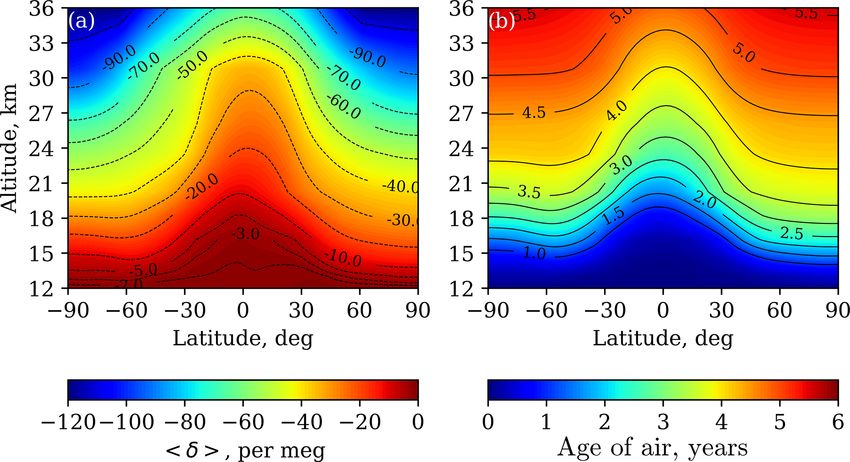
D. Belikov et al.: Modeling of gravitational separation                                                                                                     5351

2.2   Molecular diffusion                                             Here H is the atmospheric scale height, and αTi is assumed
                                                                   to be zero since the thermal diffusion effect would be of no
According to Banks and Kockarts (1973), assuming a neutral         importance in the stratosphere (Ishidoya et al., 2013). The
gas, the equation for the vertical component of the diffusion      derived flux was added to the standard transport formulation
velocity of gas 1 relative to gas 2 (w = w1 − w2 ) in a binary     for each species.
mixture of gas 1 and gas 2 in a gravitational field can be            The eddy vertical diffusion in the stratosphere is of-
written as                                                         ten neglected in CTMs. However, it should be considered

                      n2 ∂(n1 /n) M2 − M1 1 ∂p αT ∂T

                                                                   along with molecular diffusion for modeling GS. In the
w1 − w2 = −D12                   +             +        ,   (1)    SOCRATES model two options are available for the param-
                     n1 n2 ∂z        M    p ∂z   T ∂z
                                                                   eterization of the gravity wave forcing and vertical diffusion
where n1 and n2 are the concentrations of particles 1 and 2,
                                                                   coefficient (Huang et al., 1998). The default standard op-
respectively; n = n1 + n2 is the total concentration of the bi-
                                                                   tion uses the Lindzen–Holton gravity wave breaking scheme
nary mixture; T is the absolute neutral gas temperature; p is
                                                                   (Lindzen, 1981; Holton, 1982). A second option is to use the
the total pressure; M1 and M2 are the masses of particles 1
                                                                   parameterization scheme developed primarily by Fritts and
and 2; M = (n1 M1 + n2 M2 )/(n1 + n2 ) is the mean molecu-
                                                                   Lu (1993), which uses a general gravity wave spectral for-
lar mass; D12 is the molecular diffusion coefficient of gas 1
                                                                   mulation provided by the observed gravity wave spectrum to
in gas 2; and αT is the thermal diffusion factor. The three
                                                                   deduce how the gravity wave energy flux responds to vari-
terms in the brackets represent, from left to right, the effects
                                                                   ation in the background environment. The first scheme was
of concentration gradient, pressure gradient, and temperature
                                                                   adopted in the current NIES TM simulation. In general, the
gradient, respectively, on the molecular diffusion velocity.
                                                                   eddy diffusion mixes concentrations in the volume, reduces
   If component i is a multicomponent mix of minor con-
                                                                   vertical stratification, and thereby weakens the molecular dif-
stituents, then, using the hydrostatic equation, the perfect gas
                                                                   fusion effect, as discussed by Kockarts (2002).
law, and Eq. (1), the diffusion velocity wi for the ith mi-
nor constituent can be written in time-independent form (for
more details see pp. 33–34 in Banks and Kockarts, 1973):           2.3   Simulation setup

              1 ∂ni      1                1 ∂T
wi = −Di             +      + (1 + αT i )        ,           (2)   The study of GS requires considering two isotopes of atmo-
              ni ∂z     Hi                T ∂z                     spheric tracers with a small difference in molecular mass.
where Hi = kT /Mi g is the scale height, k = 1.38 ×                Following the setup for the SOCRATES baseline-atmosphere
10−23 J K−1 is the Boltzmann constant, g = 9.81 m s−2 is the       run (Ishidoya et al., 2013), we calculated the distributions
standard acceleration due to gravity for Earth, and Di is the      of 13 C16 O2 (Mi = 45) and 12 C16 O2 (Mi = 44). Firstly, a
molecular diffusion coefficient. Here also ni and αTi are the      20-year spin-up calculation with CO2 using biospheric and
number density and the thermal diffusion factor for species        oceanic fluxes only and then a 29-year (1988–2016) simu-
i, respectively.                                                   lation with total CO2 fluxes (biospheric, oceanic, and fossil
   Similar to the SOCRATES model the vertical component            fuel) were performed. The fluxes used were obtained with the
of velocity is converted to the vertical component of the          GELCA-EOF (Global Eulerian–Lagrangian Coupled Atmo-
molecular diffusion flux of a minor constituent i relative to      spheric model with Empirical Orthogonal Function) inverse
air (Huang et al., 1998):                                          modeling scheme (Zhuravlev et al., 2013). This set of fluxes
                                                                 reproduces realistic time and spatial distributions of CO2
             ∂ni    ni               ni ∂T                         mixing ratio with strong seasonal variations in the Northern
fi = −Di         +     + (1 + αT i )         .            (3)
             ∂z     Hi               T ∂z                          Hemisphere (NH) and weak variations in the Southern Hemi-
  The molecular diffusion coefficient is estimated from ki-        sphere (SH). The period 1988–2014 is covered by the orig-
netic gas theory by Banks and Kockarts (1973) to be                inal JCDAS, which is extended by JRA-55 (an updated ver-
                              s           √                        sion of the Japanese reanalysis) remapped to the same hori-
   h
        2 −1
             i
                           18   1   1        T                     zontal and vertical grid, as JCDAS production discontinued
Di cm s        = 1.52 × 10        +    ×       ,        (4)        after 2014. Use of JRA-55 for the whole simulated period
                                Mi M        n
                                                                   is preferable; however, model redevelopment is required to
where Mi and M are the mass of the minor constituent i and         take full advantage of the improved vertical and horizontal
the mean molecular mass in atomic mass units, respectively,        resolutions.
and n is the number density of air.                                   The hδi value, a measure of the GS, is defined as the iso-
   To derive a diffusive flux formulation consistent with the      topic ratio of the CO2 :
NIES model transport equation, the number density ni is sub-
stituted by the mixing ratio Ci = ni /n:                                                      h                                         i
                                                                                                    13 C16 O                12 C16 O

                                                                                           n            2          /n           2
                      1 ∂Ci  1         1       1 ∂T              hδi = δ   13 16
                                                                                 C O2       = h                                              strat
                                                                                                                                                     − 1,    (6)
fi = −Di × n × Ci            +       −     + αTi        . (5)                                   n   13 C16 O

                                                                                                                       /n   12 C16 O
                                                                                                                                        i
                      Ci ∂z      Hi H            T ∂z                                                          2                    2        trop

www.atmos-chem-phys.net/19/5349/2019/                                                       Atmos. Chem. Phys., 19, 5349–5361, 2019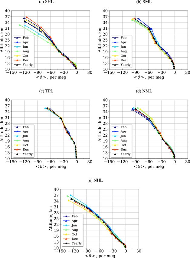
5352                                                                   D. Belikov et al.: Modeling of gravitational separation

where subscripts strat and trop denote the stratospheric and        how L−1 i distributes in the troposphere and stratosphere. Fig-
tropospheric values, respectively. As the tropospheric value        ure 2 shows the latitude–height distribution of Li−1 averaged
trop we selected the model tracer concentration from the            in each season for the case of 12 C16 O2 . Here the positive
third level, which corresponds to the lower boundary of the         values indicate that 12 C16 O2 molecules descend relative to
free troposphere. The tropospheric hδi variations are very          major constituents. The temperature fields necessary for the
small and negligible compared with those in the stratosphere.       calculation are taken from the JCDAS reanalysis. Since L−1    i
   CO2 is a useful tracer of atmospheric dynamics and trans-        is inversely proportional to temperature, it is generally small
port due to its long lifetime. It is chemically inert in the free   in the troposphere and has maxima in cold regions such as the
troposphere and has only a small stratospheric source (up to        tropical tropopause region and the winter time stratosphere.
1 ppm) from methane oxidation (Boucher et al., 2009). Suf-             The enhancement of L−1   i does not readily result in a re-
ficiently accurate estimation of emissions and sinks, together      markable GS, because it is the difference of Li−1 between
with knowledge of their trend in combination with the good          13 C16 O and 12 C16 O that creates GS in our case. We could
                                                                             2             2
performance of the NIES model in simulating greenhouse              expect that the enhancement of L−1  i combined with the long
gases, makes the selection of CO2 appropriate for this study.       stratospheric transit time in the polar stratosphere will be fa-
                                                                    vorable for GS. Figure 3 compares the horizontal distribu-
                                                                    tions of the seasonal mean hδi on 10 hPa pressure surface in
3     Results and discussion                                        polar projections. We can see remarkable GS (small values
                                                                    of hδi) in both polar regions exhibiting surprisingly clear ax-
3.1    Zonal mean distribution                                      ial symmetry. In the present analysis, the physical processes
                                                                    that drive GS (Eq. 1) have been rearranged in the form of
The zonal mean distribution of CO2 in the upper part of             Eq. (5) to separate the contribution to GS in two factors, one
the atmosphere is driven by the large-scale transport pro-          the concentration gradient (the first term) and the other the
cesses: fast quasi-isentropic mixing is combined with up-           temperature structure. A stronger seasonal variability of GS
welling in the tropics and downwelling in the extratropical         in the Southern Hemisphere is caused by changes in verti-
lowermost stratosphere. In the troposphere, vertical mixing         cal pressure gradient (Eq. 1) reflected to those in scale height
is well developed. With height, the dynamic characteristics         difference between species.
weaken, and the mass flux due to molecular diffusion in-               To minimize local temporal and spatial effects, the sea-
creases (Eq. 3). At a certain level near the tropopause, ver-       sonal variation of vertical profiles was analyzed for five main
tical mixing is no longer able to suppress diffusion and the        climate zones: the southern and northern high latitudes, the
hδi value becomes nonzero.                                          southern and northern middle latitudes, and the tropics, as
   Along with the hδi value we analyze the AoA (Fig. 1). For        shown in Table 1 and averaged over time (2000–2015). It is
this, we used the idealized linearly growing “surface” tracer       clear from Fig. 4 that seasonal variation is evident from a
proposed in the age-of-air intercomparison project (Krol            level of about 12 km, except in the tropical region, where
et al., 2018). To fit with our analysis period we extended the      it starts from 20 km. The amplitude increases with height
original simulation period (1988–2014) to 29 years (1988–           and reaches a maximum at the top of the model domain.
2016) with a shorter (10 years) spin-up, as less time is re-        It is quite obvious that seasonal variability is almost imper-
quired to reach equilibrium for the AoA analysis.                   ceptible in the tropics and increases towards the poles. The
   The processes creating the deformation of the zonal mean         maximum and minimum values are reached in December–
cross sections of the GS and the AoA are similar here: the          February and June–August for the South Pole and in April–
tropical upwelling pumps in tropospheric air and stretches          June and October–December for the North Pole, respectively.
the parameter profile upward (Fig. 1). The NIES TM re-                 Probably the stronger polar vortex in the SH presumably
sults shows strong subtropical mixing barriers in both hemi-        leads to the enhanced GS (smaller values of hδi) in JJA in the
spheres compared with the SOCRATES model.                           SH (Figs. 3a and 4a light blue line) compared to that in DJF
   To estimate the contribution of atmospheric conditions to        in the NH (Figs. 3c and 4e). In the NH, on the other hand,
molecular diffusion, we consider the sum of the three terms         GS appears weakest during winter (Fig. 3c) in spite of the
in the square bracket of Eq. (5). Because the contribution of       enhancement of L−1  i (Fig. 2c).
the first term (concentration gradient) is relatively small, the       Weak sensitivity to seasonal changes of the tracer concen-
second term (originated from pressure gradient in Eq. 1) is         tration is a significant advantage of GS over AoA, which is
the major contributor among the three terms. Therefore, the         the standard indicator of circulation in the stratosphere. On
sum of the three terms can be approximated by the difference        the other hand, this method requires more accurate sampling
between the reciprocals of two scale heights (hereafter re-         tools (i.e., balloon-borne cryogenic samplers) that are more
ferred to as L−1
               i ). It has a dimension reciprocal to the length     difficult to deploy than other more common methods.
and is interpreted as a measure of the efficiency of vertical
molecular diffusion under gravity. In view of the essentially
one-dimensional nature of GS, it is interesting to consider

Atmos. Chem. Phys., 19, 5349–5361, 2019                                              www.atmos-chem-phys.net/19/5349/2019/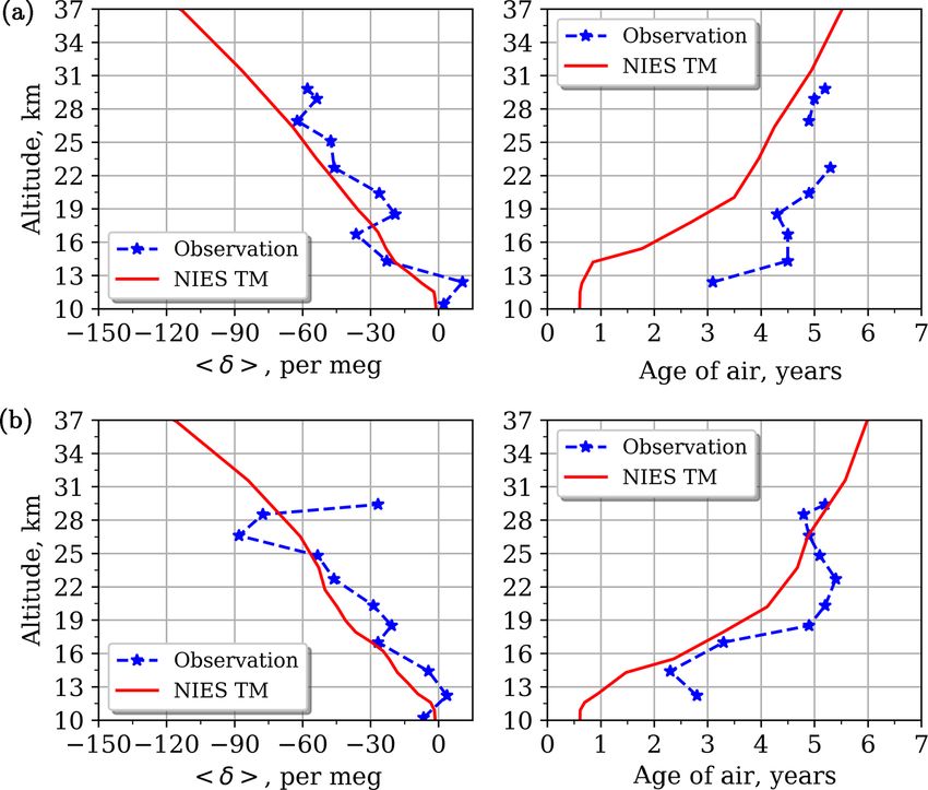
D. Belikov et al.: Modeling of gravitational separation                                                                             5353

Figure 1. Annual mean altitude–latitude distributions of hδi value (per meg) (a) and the AoA (years) (b) calculated using the NIES TM. The
unit (per meg) is typically used in isotope analysis and is the same as 10−3 ‰.

Figure 2. Mean altitude–latitude distributions of the difference between the reciprocals of Hi and H (L−1     −1
                                                                                                       i [1 km ], see text) for (a) JJA,
(b) SON, (c) DJF, and (d) MAM. The results are averaged for 2000–2015.

www.atmos-chem-phys.net/19/5349/2019/                                                    Atmos. Chem. Phys., 19, 5349–5361, 2019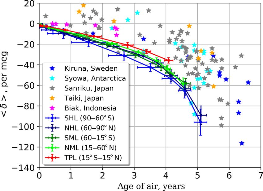
5354                                                                        D. Belikov et al.: Modeling of gravitational separation

Figure 3. Mean latitude–longitude distributions of hδi value at the 10 hPa level in south polar and north polar projections for (a) JJA, (b)
SON, (c) DJF, and (d) MAM. The results are averaged for 2000–2015.

Table 1. Latitude bands used for averaging hδi values.

                                  Number     Short name     Long name                    Latitude interval
                                  1          SHL            Southern high latitudes      90◦ S–60◦ S
                                  2          SML            Southern middle latitudes    60◦ S–15◦ S
                                  3          TPL            Tropical latitudes           15◦ S–15◦ N
                                  4          NML            Northern middle latitudes    15◦ N–60◦ N
                                  5          NHL            Northern high latitudes      60◦ N–90◦ N

3.2    Vertical profiles                                                on the atmospheric component, as follows from Eq. 6. Thus
                                                                        δ values from observations of various tracers and the current
                                                                        simulations can be compared.
The modeled results are compared with measurements over
                                                                           Most of the observations were collected in the northern
the main climatic zones: the circumpolar regions, the temper-
                                                                        part of Japan over Sanriku (eight profiles) and Taiki (one) in
ate latitudes, and the tropical latitudes (Table 2). The collec-
                                                                        the warm season. Five profiles were observed at the begin-
tion of stratospheric air samples using a balloon-borne cryo-
                                                                        ning of summer (late May to early June) and four profiles at
genic sampler was initiated in 1985 at the Sanriku Balloon
                                                                        the end of summer (late August to early September). Typical
Center of the Institute of Space and Astronautical Science
                                                                        spring and fall profiles are shown in Fig. 5. For this com-
(Nakazawa et al., 1995, 2002; Aoki et al., 2003; Goto et al.,
                                                                        parison, the modeled data are daily output at the nearest grid
2017; Sugawara et al., 2018; Hasebe et al., 2018). The pro-
                                                                        cell.
gram has continued up to the present. In addition to obser-
                                                                           In the NH, the tropospheric CO2 is dominated by a strong
vations over Japan, stratospheric air samples were also col-
                                                                        seasonal cycle due to biospheric activity, which removes CO2
lected over the Scandinavian Peninsula, Antarctica, and In-
                                                                        by photosynthesis during the growing phase to reach a min-
donesia.
                                                                        imum in August–September and releases it during boreal
   From those air samples, δ(15 N) of N2 , δ(18 O) of O2 ,
                                                                        autumn and winter with a maximum in April–May. Due to
δ(O2 /N2 ), δ(Ar/N2 ), and δ(40 Ar) were derived to detect GS
                                                                        steady growth and seasonal variation, CO2 concentrations in
in the stratosphere (Ishidoya et al., 2006, 2008, 2013). The
                                                                        the atmosphere contain both monotonically increasing and
effect of GS on the isotopic ratio depends on 1m rather than

Atmos. Chem. Phys., 19, 5349–5361, 2019                                                    www.atmos-chem-phys.net/19/5349/2019/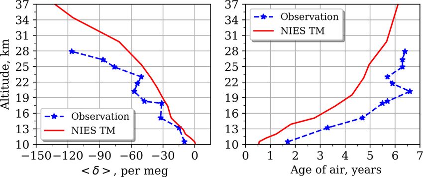
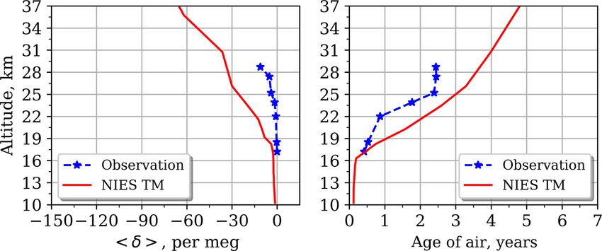
D. Belikov et al.: Modeling of gravitational separation                                                                       5355

Figure 4. Profiles of hδi calculated by the model for February, April, June, August, October, December, and yearly mean averaged for
2000–2015 over the five latitudinal bands shown in Table 1

periodic signals. Spring profiles are smoother, while in au-           For the high-latitude sites Kiruna and Syowa (Figs. 6–7)
tumn they vary with height. The observed AoA shows a                the observed profiles are mainly smooth and have smaller
strong inversion in the lower altitudes due to seasonal up-         vertical fluctuation, apart from the uppermost level over the
take of CO2 , as confirmed by CONTRAIL measurements                 Syowa station for 5 January 2004.
(Machida et al., 2008; Sawa et al., 2008) and the Lagrangian           Due to the limited availability of balloon launching facili-
transport model TRACZILLA (Diallo et al., 2017). The AoA            ties, only one air sample has been conducted in the equatorial
calculated from the modeled surface tracer does not repro-          mid-stratosphere over Biak (Hasebe et al., 2018). The ob-
duce such effect.                                                   served distribution can be explained by the mixing of large-

www.atmos-chem-phys.net/19/5349/2019/                                                Atmos. Chem. Phys., 19, 5349–5361, 2019
5356                                                                           D. Belikov et al.: Modeling of gravitational separation

Table 2. Observation sites.

                       Number      Site name             Site coordinates      Observation dates
                       1           Biak, Indonesia       (1◦ S, 136◦ E)        22–28 Feb 2015
                       2           Kiruna, Sweden        (68◦ N, 21◦ E)        18 Mar 1997
                       3           Sanriku, Japan        (39◦ N, 142◦ E)       8 Jun 1995, 31 May 1999, 28 Aug 2000,
                                                                               30 May 2001, 4 Sep 2002, 6 Sep 2004,
                                                                               3 Jun 2006, and 4 Jun 2007
                       4           Syowa, Antarctica     (69◦ S, 39◦ E)        3 Jan 1998 and 5 Jan 2004
                       5           Taiki, Japan          (43◦ N, 143◦ E)       22 Aug 2010

Figure 5. Vertical profiles over Sanriku of hδi (per meg) (a, c) and AoA (years) (b, d) calculated from the modeled “surface” tracer (in red)
and the observed CO2 (in blue) distributions for 4 June 2007 (a, b) and 28 August 2000 (c, d).

scale NH and SH background values and long-range tracer                     and r(hδi), respectively), and the Pearson correlation coeffi-
transport with convective lifting (Inai et al., 2018). For this             cient between AoA and hδi from observation (r(AoA, hδi)o )
site, the hδi value and the AoA variations with height are                  and from the model (r(AoA, hδi)m ). To calculate standard
very small (Fig. 8), as vertical upwelling pumps young and                  deviation and correlation coefficients only coincident points
well-mixed air upward.                                                      were selected.
    Although this is not a model validation paper, it is nec-                  The high values of the correlation coefficients between
essary to evaluate the modeled results by comparison with                   simulated and observed parameters prove the model effi-
observations, as the new parameterization for GS simula-                    ciency with the implemented parameterization. The lower
tion was incorporated in the NIES TM. A detailed statis-                    correlation for GS than for r(AoA) stresses the complexity
tical analysis is summarized for the five observational sites               of the high-precision cryogenic sampling required for GS.
in Table 3. This includes the standard deviation of the mis-                For example, most observed profiles show a tendency to have
fit between modeled and observed AoA and hδi (σ (1AoA)                      zones of very weak increase or even inversion of the param-
and σ (1hδi), respectively), the Pearson correlation coeffi-                eters starting from a level of 20–25 km. Despite these lim-
cient between modeled and observed AoA and hδi (r(AoA)                      itations, the ability to study the physics underlying GS is a

Atmos. Chem. Phys., 19, 5349–5361, 2019                                                      www.atmos-chem-phys.net/19/5349/2019/
D. Belikov et al.: Modeling of gravitational separation 5357
Figure 6. Same as Fig. 5 but over the Kiruna site for 18 March 1997.
Figure 7. Same as Fig. 5 but over the Syowa station for 3 January 1998 (a) and 5 January 2004 (b).
fundamental advantage of the 3-D simulation compared with one value increases with height and the other decreases, the
the 2-D simulation as performed by SOCRATES. correlation is negative. Modeled results show stronger anti-
The standard deviations σ (AoA) and σ (hδi) quantify correlation than that observed, probably due to more straight-
model–observation misfits. We stress a tendency of increase forward connections in transport simulation; the parameteri-
towards the high latitudes, although it seems that a larger gap zation used may not take into account additional factors af-
is obtained for Biak. However, if we normalize the standard fecting GS. We also do not exclude the influence of observa-
deviations by the value of the absolute maximum value of the tional errors.
characteristic, the error decreases towards high latitudes.
GS and AoA are useful indicators of atmospheric trans- 3.3 Relationship between age of air and hδi
port processes. Two other correlations from Table 3 (r(AoA,
hδi)o and r(AoA, hδi)m ) quantify their relationship. Since Further study of the relationship between the AoA and the
hδi value is useful for understanding the atmospheric pro-
www.atmos-chem-phys.net/19/5349/2019/ Atmos. Chem. Phys., 19, 5349–5361, 20195358 D. Belikov et al.: Modeling of gravitational separation
Figure 8. Same as Fig. 5 but over the Biak site for 22–28 February 2015.
Table 3. Standard deviation of misfit between modeled and observed AoA and hδi value (σ (1AoA) and σ (1hδi), respectively); the Pearson
correlation coefficient between modeled and observed AoA and hδi value (r(AoA) and r(hδi), respectively); the Pearson correlation coefficient
between AoA and hδi from observation (r(AoA, hδi)o ) and from the model (r(AoA, hδi)m ).
Number Site name σ (1AoA), yr σ (1hδi), per meg r(AoA) r(hδi) r(AoA, hδi)o r(AoA, hδi)m
1 Biak, Indonesia 0.47 10.33 0.95 0.96 –0.77 –0.92
2 Kiruna, Sweden 0.67 15.55 0.89 0.76 –0.74 –0.96
3 Sanriku, Japan 0.44 8.62 0.97 0.94 –0.86 –0.96
4 Syowa, Antarctica 0.84 15.76 0.86 0.78 –0.75 –0.95
5 Taiki, Japan 0.63 9.27 0.91 0.84 –0.79 –0.99
cesses, as both would be affected to some extent by changes sonal variation. For younger air (0–2 years) the seasonal vari-
in the stratospheric circulation. For comparison the modeled ability of AoA is maximal and falls with altitude, while the
AoA and hδi values were averaged over the same five broad- hδi variability increases continuously upwards, as described
latitude bands as in Sect. 3.1 (see Table 1). Along with the in Sect. 3.1.
modeled values (solid lines) the observed data are also de- Sugawara et al. (2018) assumed that vertical upwelling
picted (symbols) in Fig. 9. Observation sites are quite evenly in he tropical tropopause layer (TTL) acts to weaken and
distributed across the selected latitude bands: Syowa in the downwelling in high latitudes acts to strengthen the effect
southern high latitudes, Biak in the tropics, Sanriku and Taiki on the GS. To minimize the discrepancy between the model-
in the northern middle latitudes, and Kiruna in the northern calculated (with SOCRATES) and observed hδi values over
high latitudes. the equatorial region, a correction of the mean meridional cir-
Figure 9 shows a near-one-to-one relationship between culation and the horizontal eddy diffusivity was performed.
AoA and GS regardless of latitude and height. Although the However, that correction cannot fully improve the simulation
model–observation discrepancy is significant for all layers, of the stratospheric circulation and hence the reproducibil-
the distributions of observations show a similar pattern for ity of AoA and GS by the SOCRATES model. In this study
the lower part of the stratosphere despite large scatter. The the tracer simulation is based on reanalysis, which describes
positive hδi values obtained from observations are not repro- the atmospheric circulation in sufficient detail. As part of the
ducible according to the theory. global balanced air transport the upwelling and downwelling
The hδi value decreases rapidly for age values older than are limited by various constraints including mass flux conser-
4 years, as the molecular diffusion coefficient increases with vation. The resulting tracer field distribution simultaneously
increasing height due to its pressure dependence (Eq. 4), describes AoA and GS, so both parameters can be used to
which causes the enhancement of gravitational separation describe the structure of the global atmospheric circulation.
with increasing height. This mechanism does not affect AoA However, the limited set of observations and the limitations
significantly in the stratosphere (Ishidoya et al., 2008, 2013; of the model do not yet allow us to investigate this mecha-
Sugawara et al., 2018). This emphasizes a nonlinearity in the nism and determine the structure of the AoA–GS relationship
GS–AoA relationship in the stratosphere. in more detail.
Another difference stressed the independence of the driv- Chabrillat et al. (2018) presented a consistent intercom-
ing mechanisms of AoA, and GS is the influence of the sea- parison of AoA according to five modern reanalyses (ERA-
Atmos. Chem. Phys., 19, 5349–5361, 2019 www.atmos-chem-phys.net/19/5349/2019/D. Belikov et al.: Modeling of gravitational separation 5359
to reproduce the mean value and the number of small-scale
fluctuations recorded by high-precision cryogenic balloon-
borne observations in the lower stratosphere. This recon-
struction suggests that the tracer distribution can be ex-
plained by the properties of transport, as resolved by meteo-
rological reanalysis and the representation of sub-grid-scale
effects as diffusion. Overall, the implemented molecular dif-
fusion parameterization in the NIES TM shows reasonable
performance.
We found a strong relationship between the modeled GS
and AoA, which is the main indicator of circulation in the
stratosphere. However, in contrast to AoA, the GS has a
lower sensitivity to seasonal variability, which is a signif-
icant issue in studies of atmospheric circulation. Thus, the
modeled GS characteristics can provide useful insights and
complement AoA information to give a more comprehensive
Figure 9. Plot of hδi value against AoA. The modeled results are evaluation of structure changes in the UTLS. However, due to
averaged for the five latitudinal bands shown in Table 1 and over
the simplified approach and parameterizations, the presented
time for 2000–2015. Symbols represent all available observations
for Kiruna, Syowa, Sanriku, Taiki, and Biak sites. Error bar values
simulation of the GS using the NIES model could not fully
correspond to 1σ . achieve the potential of 3-D modeling. Modern reanalysis
dataset and recently developed transport models that effec-
tively simulated the upper atmosphere can be employed to
Interim, JRA-55, MERRA, MERRA-2, and CFSR) and address these issues. Since this work is the first in 3-D mod-
found significant diversity in the distributions which were eling of GS, we believe this insight is useful for the scientific
obtained with the BASCOE (Belgian Assimilation System community working in the field of the UTLS studies.
for Chemical Observations) transport model, depending on
the input reanalysis. They have also found large disagree-
ment between the five reanalyses with respect to the long- Code and data availability. Additional data requests should be ad-
dressed to Dmitry Belikov (dmitry.belikov@ees.hokudai.ac.jp).
term trends of AoA. Thus, an ambitious multi-reanalyses ap-
proach is needed to distinguish what is robust in the current
GS results from what is not.
Author contributions. DB carried out the NIES model simulations
and the data analysis. SS, SI and FH contributed to the design of the
analysis and theoretical description of the GS process. SM prepared
4 Conclusions the reanalysis data and contributed code of the NIES TM. SA, SM
and TK provided the observational data. SS, SI, FH, SM, SA, SM
A three-dimensional simulation of GS in the UTLS zone and TK provided helpful discussion and comments. DB wrote the
is performed for the first time using the NIES TM with a manuscript with contributions from all co-authors.
molecular diffusion parameterization. We consider the hδi
values derived from the distribution of two isotopes 12 C16 O2
and 13 C16 O2 . The modeled hδi values are compared to ob- Competing interests. The authors declare that they have no conflict
servations and the zonal mean distributions from the two- of interest.
dimensional SOCRATES model.
In comparison with the SOCRATES simulation, the NIES
model has a number of significant advantages: a three- Acknowledgements. We sincerely thank the balloon engineering
dimensional tracer transport simulation driven by global JC- group of the Institute of Space and Astronautical Science JAXA
DAS reanalysis and a vertical coordinate with isentropic lev- for their cooperation in our stratospheric air sampling. This work
els. The model is optimized to run the greenhouse gas sim- is partly supported by the Japan Society for Promotion of Sci-
ulation, as confirmed through various validation and multi- ence, Grant-in-Aid for Scientific Research (S) 26220101. We thank
Masatomo Fujiwara, associated Professor at Hokkaido University
model inter-comparisons. The use of optimized CO2 fluxes
for useful comments regarding the GS studies.
provided realistic tracer distribution and seasonality. Along
with these strengths, some weaknesses are also revealed:
coarse vertical resolution and the shallow top of the model Review statement. This paper was edited by Peter Haynes and re-
domain. viewed by two anonymous referees.
The model-to-observation comparison shows that the
model with this molecular diffusion parameterization is able
www.atmos-chem-phys.net/19/5349/2019/ Atmos. Chem. Phys., 19, 5349–5361, 20195360 D. Belikov et al.: Modeling of gravitational separation
References Engel, A., Möbius, T., Bönisch, H., Schmidt, U., Heinz, R., Levin,
I., Atlas, E., Aoki, S., Nakazawa, T., Sugawara, S., Moore, F.,
Aoki, S., Nakazawa, T., Machida, T., Sugawara, S., Morimoto, S., Hurst, D., Elkins, J., Schauffler, S., Andrews, A., and Boering,
Hashida, G., Yamanouchi, T., Kawamura, K., and Honda, H.: K.: Age of stratospheric air unchanged within uncertainties over
Carbon dioxide variations in the stratosphere over Japan, Scan- the past 30 years, Nat. Geosci., 2, 28–31, 2009.
dinavia and Antarctica, Tellus B, 55, 178–186, 2003. Field, C. B., Barros, V. R., Mach, K., and Mastrandrea, M.: Cli-
Austin, P. M. and Houze Jr., R. A.: A technique for computing ver- mate change 2014: impacts, adaptation, and vulnerability, Vol. 1,
tical transports by precipitating cumuli, J. Atmos. Sci., 30, 1100– Cambridge University Press Cambridge and New York, p. 1140,
1111, 1973. 2014.
Banks, P. and Kockarts, G.: Aeronomy, Academic, New York, Fritts, D. C. and Lu, W.: Spectral estimates of gravity wave energy
ISBN: 9781483260068, Academic Press, 372 pp., 1973. and momentum fluxes, Part II: Parameterization of wave forcing
Belikov, D. A., Maksyutov, S., Krol, M., Fraser, A., Rigby, M., and variability, J. Atmos. Sci., 50, 3695–3713, 1993.
Bian, H., Agusti-Panareda, A., Bergmann, D., Bousquet, P., Garcia, R. R. and Randel, W. J.: Acceleration of the Brewer–Dobson
Cameron-Smith, P., Chipperfield, M. P., Fortems-Cheiney, A., circulation due to increases in greenhouse gases, J. Atmos. Sci.,
Gloor, E., Haynes, K., Hess, P., Houweling, S., Kawa, S. R., 65, 2731–2739, 2008.
Law, R. M., Loh, Z., Meng, L., Palmer, P. I., Patra, P. K., Garfinkel, C. I., Aquila, V., Waugh, D. W., and Oman, L. D.:
Prinn, R. G., Saito, R., and Wilson, C.: Off-line algorithm Time-varying changes in the simulated structure of the Brewer–
for calculation of vertical tracer transport in the troposphere Dobson Circulation, Atmos. Chem. Phys., 17, 1313–1327,
due to deep convection, Atmos. Chem. Phys., 13, 1093–1114, https://doi.org/10.5194/acp-17-1313-2017, 2017.
https://doi.org/10.5194/acp-13-1093-2013, 2013a. Gettelman, A., Hoor, P., Pan, L. L., Randel, W. J., Heg-
Belikov, D. A., Maksyutov, S., Sherlock, V., Aoki, S., Deutscher, glin, M. I., and Birner, T.: The extratropical upper tropo-
N. M., Dohe, S., Griffith, D., Kyro, E., Morino, I., Nakazawa, T., sphere and lower stratosphere, Rev. Geophys., 49, RG3003,
Notholt, J., Rettinger, M., Schneider, M., Sussmann, R., Toon, https://doi.org/10.1029/2011RG000355, 2011.
G. C., Wennberg, P. O., and Wunch, D.: Simulations of column- Goto, D., Morimoto, S., Aoki, S., Sugawara, S., Ishidoya, S., Inai,
averaged CO2 and CH4 using the NIES TM with a hybrid sigma- Y., Toyoda, S., Honda, H., Hashida, G., Yamanouchi, T., and
isentropic (σ − 2) vertical coordinate, Atmos. Chem. Phys., 13, Nakazawa, T.: Vertical profiles and temporal variations of green-
1713–1732, https://doi.org/10.5194/acp-13-1713-2013, 2013b. house gases in the stratosphere over Syowa Station, Antarctica,
Boucher, O., Friedlingstein, P., Collins, B., and Shine, K. P.: SOLA, 13, 224–229, 2017.
The indirect global warming potential and global temperature Grell, G. A., Dudhia, J., and Stauffer, D. R.: A description of
change potential due to methane oxidation, Environ. Res. Lett., the fifth-generation Penn State/NCAR mesoscale model (MM5),
4, 044007, https://doi.org/10.1088/1748-9326/4/4/044007, 2009. NCAR Tech. Note, p. 122, 1995.
Butchart, N.: The Brewer-Dobson circulation, Rev. Geophys., 52, Hack, J. J., Boville, B. A., Briegleb, B. P., Kiehl, J. T., Rasch, P. J.,
157–184, 2014. and Williamson, D. L.: Description of the NCAR community cli-
Butchart, N., Scaife, A., Bourqui, M., De Grandpré, J., Hare, S., mate model (CCM2), NCAR Tech. Note, 382, p. 120, 1993.
Kettleborough, J., Langematz, U., Manzini, E., Sassi, F., Shibata, Hall, T. M. and Plumb, R. A.: Age as a diagnostic of strato-
K., Shindell, D., and Sigmond, M.: Simulations of anthropogenic spheric transport, J. Geophys. Res.-Atmos., 99, 1059–1070,
change in the strength of the Brewer–Dobson circulation, Clim. https://doi.org/10.1029/93JD03192, 1994.
Dynam., 27, 727–741, 2006. Hasebe, F., Aoki, S., Morimoto, S., Inai, Y., Nakazawa, T., Sug-
Chabrillat, S., Vigouroux, C., Christophe, Y., Engel, A., Errera, Q., awara, S., Ikeda, C., Honda, H., Yamazaki, H., Halimurrahman,
Minganti, D., Monge-Sanz, B. M., Segers, A., and Mahieu, E.: Komala, N., Putri, F. A., Budiyono, A., Soedjarwo, M., Ishi-
Comparison of mean age of air in five reanalyses using the BAS- doya, S., Toyoda, S., Shibata, T., Hayashi, M., Eguchi, N., Nishi,
COE transport model, Atmos. Chem. Phys., 18, 14715–14735, N., Fujiwara, M., Ogino, S.-Y., Shiotani, M., and Sugidachi, T.:
https://doi.org/10.5194/acp-18-14715-2018, 2018. Coordinated Upper-troposphere-to-stratosphere Balloon Experi-
Chapman, S. and Milne, E.: The composition, ionisation and vis- ment in Biak (CUBE/Biak), B. Am. Meteorol. Soc., 99, 1213–
cosity of the atmosphere at great heights, Q. J. Roy. Meteorol. 1230, 2018.
Soc., 46, 357–398, 1920. Hegglin, M. I., Plummer, D. A., Shepherd, T. G., Scinocca, J. F.,
Dee, D. P., Uppala, S. M., Simmons, A., Berrisford, P., Poli, P., Anderson, J., Froidevaux, L., Funke, B., Hurst, D., Rozanov,
Kobayashi, S., Andrae, U., Balmaseda, M., Balsamo, G., Bauer, A., Urban, J., von Clarmann, T., Walker, K. A., Wang, H. J.,
D. P., Bechtold, P., M. Beljaars, A. C., van de Berg, L., Bidlot, Tegtmeier, S., and Weigel, K.: Vertical structure of stratospheric
J., Bormann, N., Delsol, C., Dragani, R., Fuentes, M., Geer, A. water vapour trends derived from merged satellite data, Nat.
J., Haimberger, L.„ Healy, Hersbah, H., Hólm, E. V., Isaksen, L., Geosci., 7, 768–776, 2014.
Kållberg, P., Köhler, M., Matricardi, M., McNally, A. P., Monge- Hegglin, M. I., Gettelman, A., Hoor, P., Krichevsky, R., Manney,
Sanz, B. M., Morcrette, J.-J., Park, B.-K., Peubey, C., de Rosnay, G. L., Pan, L. L., Son, S.-W., Stiller, G., Tilmes, S., Walker,
P., Tavolato, C., Thépaut, J.-N., and Vitart, F.: The ERA-Interim K. A., Eyring, V., Shepherd, T. G., Waugh, D., Akiyoshi, H.,
reanalysis: Configuration and performance of the data assimila- Añel, J. A., Austin, J., Baumgaertner, A., Bekki, S., Braesicke, P.,
tion system, Q. J. Roy. Meteorol. Soc., 137, 553–597, 2011. Brühl, C., Butchart, N., Chipperfield, M., Dameris, M., Dhomse,
Diallo, M., Legras, B., Ray, E., Engel, A., and Añel, J. A.: S., Frith, S., Garny, H., Hardiman, S. C., Jöckel, P., Kinnison,
Global distribution of CO2 in the upper troposphere D. E., Lamarque, J. F., Mancini, E., Michou, M., Morgenstern,
and stratosphere, Atmos. Chem. Phys., 17, 3861–3878, O., Nakamura, T., Olivié, D., Pawson, S., Pitari, G., Plummer,
https://doi.org/10.5194/acp-17-3861-2017, 2017.
Atmos. Chem. Phys., 19, 5349–5361, 2019 www.atmos-chem-phys.net/19/5349/2019/D. Belikov et al.: Modeling of gravitational separation 5361 D. A., Pyle, J. A., Rozanov, E., Scinocca, J. F., Shibata, K., Maksyutov, S. and Inoue, G.: Vertical profiles of radon and CO2 Smale, D., Teyssèdre, H., Tian, W., and Yamashita, Y.: Mul- simulated by the global atmospheric transport model, CGER re- timodel assessment of the upper troposphere and lower strato- port, CGER-I039-2000, CGER, NIES, Japan, 7, 39–41, 2000. sphere: Extratropics, J. Geophys. Res.-Atmos., 115, D00M09, Nakazawa, T., Machida, T., Sugawara, S., Murayama, S., Mori- https://doi.org/10.1029/2010JD013884, 2010. moto, S., Hashida, G., Honda, H., and Itoh, T.: Measurements Holton, J. R.: The role of gravity wave induced drag and diffusion of the stratospheric carbon dioxide concentration over Japan us- in the momentum budget of the mesosphere, J. Atmos. Sci., 39, ing a Balloon-borne cryogenic sampler, Geophys. Res. Lett., 22, 791–799, 1982. 1229–1232, https://doi.org/10.1029/95gl01188,1995. Huang, T., Walters, S., Brasseur, G., Hauglustaine, D., and Wu, Nakazawa, T., Aoki, S., Kawamura, K., Saeki, T., Sugawara, S., W.: Description of SOCRATES: A chemical dynamical radiative Honda, H., Hashida, G., Morimoto, S., Yoshida, N., Toyoda, S., two-dimensional model, NCAR, p. 94, 1998. and Makide, Y.: Variations of stratospheric trace gases measured Inai, Y., Aoki, S., Honda, H., Furutani, H., Matsumi, Y., Ouchi, using a balloon-borne cryogenic sampler, Adv. Space Res., 30, M., Sugawara, S., Hasebe, F., Uematsu, M., and Fujiwara, M.: 1349–1357, 2002. Balloon-borne tropospheric CO2 observations over the equato- Onogi, K., Tsutsui, J., Koide, H., Sakamoto, M., Kobayashi, S., Hat- rial eastern and western Pacific, Atmos. Environ., 184, 24–36, sushika, H., Matsumoto, T., Yamazaki, N., Kamahori, H., Taka- 2018. hashi, K., and Kadokura, S.: The JRA-25 reanalysis, J. Meteorol. Ishidoya, S., Sugawara, S., Hashida, G., Morimoto, S., Soc. Jpn. Ser. II, 85, 369–432, 2007. Aoki, S., Nakazawa, T., and Yamanouchi, T.: Verti- Ray, E. A., Moore, F. L., Rosenlof, K. H., Davis, S. M., Sweeney, cal profiles of the O2 /N2 ratio in the stratosphere over C., Tans, P., Wang, T., Elkins, J. W., Bönisch, H., Engel, A., and Japan and Antarctica, Geophys. Res. Lett., 33, L13701, Sugawara, S.: Improving stratospheric transport trend analysis https://doi.org/10.1029/2006GL025886, 2006. based on SF6 and CO2 measurements, J. Geophys. Res.-Atmos., Ishidoya, S., Sugawara, S., Morimoto, S., Aoki, S., and Nakazawa, 119, 14110–14128, 2014. T.: Gravitational separation of major atmospheric components of Sawa, Y., Machida, T., and Matsueda, H.: Seasonal vari- nitrogen and oxygen in the stratosphere, Geophys. Res. Lett., 35, ations of CO2 near the tropopause observed by com- L03811, https://doi.org/10.1029/2007GL030456, 2008. mercial aircraft, J. Geophys. Res.-Atmos., 113, D23301, Ishidoya, S., Sugawara, S., Morimoto, S., Aoki, S., Nakazawa, T., https://doi.org/10.1029/2008JD010568, 2008. Honda, H., and Murayama, S.: Gravitational separation in the Stiller, G. P., von Clarmann, T., Haenel, F., Funke, B., Glatthor, N., stratosphere – a new indicator of atmospheric circulation, At- Grabowski, U., Kellmann, S., Kiefer, M., Linden, A., Lossow, S., mos. Chem. Phys., 13, 8787–8796, https://doi.org/10.5194/acp- and López-Puertas, M.: Observed temporal evolution of global 13-8787-2013, 2013. mean age of stratospheric air for the 2002 to 2010 period, At- Kockarts, G.: Aeronomy, a 20th Century emergent science: the role mos. Chem. Phys., 12, 3311–3331, https://doi.org/10.5194/acp- of solar Lyman series, Ann. Geophys., 20, 585–598, 2002. 12-3311-2012, 2012. Krol, M., de Bruine, M., Killaars, L., Ouwersloot, H., Pozzer, Sugawara, S., Ishidoya, S., Aoki, S., Morimoto, S., Nakazawa, T., A., Yin, Y., Chevallier, F., Bousquet, P., Patra, P., Be- Toyoda, S., Inai, Y., Hasebe, F., Ikeda, C., Honda, H., Goto, D., likov, D., Maksyutov, S., Dhomse, S., Feng, W., and Chip- and Putri, F. A.: Age and gravitational separation of the strato- perfield, M. P.: Age of air as a diagnostic for transport spheric air over Indonesia, Atmos. Chem. Phys., 18, 1819–1833, timescales in global models, Geosci. Model Dev., 11, 3109– https://doi.org/10.5194/acp-18-1819-2018, 2018. 3130, https://doi.org/10.5194/gmd-11-3109-2018, 2018. Tiedtke, M.: A comprehensive mass flux scheme for cumulus pa- Leedham Elvidge, E., Bönisch, H., Brenninkmeijer, C. A. M., En- rameterization in large-scale models, Mon. Weather Rev., 117, gel, A., Fraser, P. J., Gallacher, E., Langenfelds, R., Mühle, 1779–1800, 1989. J., Oram, D. E., Ray, E. A., Ridley, A. R., Röckmann, T., Warneck, P. and Williams, J.: The atmospheric Chemist’s compan- Sturges, W. T., Weiss, R. F., and Laube, J. C.: Evaluation ion: numerical data for use in the atmospheric sciences, Springer of stratospheric age of air from CF4 , C2 F6 , C3 F8 , CHF3 , Science & Business Media, 2012. HFC-125, HFC-227ea and SF6 ; implications for the calcu- Waugh, D. and Hall, T.: Age of stratospheric air: theory, lations of halocarbon lifetimes, fractional release factors and observations, and models, Rev. Geophys., 40, p. 1010, ozone depletion potentials, Atmos. Chem. Phys., 18, 3369–3385, https://doi.org/10.1029/2000RG000101, 1010, 2002. https://doi.org/10.5194/acp-18-3369-2018, 2018. Zhuravlev, R., Ganshin, A., Maksyutov, S. S., Oshchepkov, S., and Li, F., Austin, J., and Wilson, J.: The strength of the Brewer–Dobson Khattatov, B.: Estimation of global CO2 fluxes using ground- circulation in a changing climate: Coupled chemistry–climate based and satellite (GOSAT) observation data with empirical or- model simulations, J. Clim., 21, 40–57, 2008. thogonal functions, Atmos. Ocean. Opt., 26, 507–516, 2013. Lindzen, R. S.: Turbulence and stress owing to gravity wave and tidal breakdown, J. Geophys. Res.-Ocean., 86, 9707–9714, 1981. Machida, T., Matsueda, H., Sawa, Y., Nakagawa, Y., Hirotani, K., Kondo, N., Goto, K., Nakazawa, T., Ishikawa, K., and Ogawa, T.: Worldwide measurements of atmospheric CO2 and other trace gas species using commercial airlines, J. Atmos. Ocean. Tech- nol., 25, 1744–1754, 2008. www.atmos-chem-phys.net/19/5349/2019/ Atmos. Chem. Phys., 19, 5349–5361, 2019
You can also read