Climate impact of Finnish air pollutants and greenhouse gases using multiple emission metrics
←
→
Page content transcription
If your browser does not render page correctly, please read the page content below

Atmos. Chem. Phys., 19, 7743–7757, 2019
https://doi.org/10.5194/acp-19-7743-2019
© Author(s) 2019. This work is distributed under
the Creative Commons Attribution 4.0 License.

Climate impact of Finnish air pollutants and greenhouse gases using
multiple emission metrics
Kaarle Juhana Kupiainen1 , Borgar Aamaas2 , Mikko Savolahti1 , Niko Karvosenoja1 , and Ville-Veikko Paunu1
1 Finnish   Environment Institute, Mechelininkatu 34a, P.O. Box 140, 00251 Helsinki, Finland
2 CICERO     Center for International Climate Research, PB 1129 Blindern, 0318 Oslo, Norway

Correspondence: Kaarle Juhana Kupiainen (kaarle.kupiainen@ym.fi, kaarle.kupiainen@ymparisto.fi)

Received: 11 October 2018 – Discussion started: 13 December 2018
Revised: 26 March 2019 – Accepted: 6 May 2019 – Published: 11 June 2019

Abstract. We present a case study where emission metric             of BC emissions is enhanced during winter. Many metric
values from different studies are applied to estimate global        choices are available, but our findings hold for most choices.
and Arctic temperature impacts of emissions from a north-
ern European country. This study assesses the climate im-
pact of Finnish air pollutants and greenhouse gas emissions
from 2000 to 2010, as well as future emissions until 2030.          1   Introduction
We consider both emission pulses and emission scenarios.
The pollutants included are SO2 , NOx , NH3 , non-methane           The Paris Agreement and its target of “holding the increase
volatile organic compound (NMVOC), black carbon (BC),               in the global average temperature to well below 2 ◦ C above
organic carbon (OC), CO, CO2 , CH4 and N2 O, and our study          pre-industrial levels and pursuing efforts to limit the tem-
is the first one for Finland to include all of them in one coher-   perature increase to 1.5 ◦ C above pre-industrial levels” (UN-
ent dataset. These pollutants have different atmospheric life-      FCCC, 2015) provides an important framework for individ-
times and influence the climate differently; hence, we look at      ual countries to consider the climate impacts and mitigation
different climate metrics and time horizons. The study uses         possibilities of its emissions. Globally, CO2 and greenhouse
the global warming potential (GWP and GWP∗ ), the global            gas emissions are key components in achieving the targets
temperature change potential (GTP) and the regional temper-         of the agreement, but the role of short-lived climate forcers
ature change potential (RTP) with different timescales for es-      (SLCFs) should also be studied as additional drivers of the
timating the climate impacts by species and sectors globally        surface temperatures. The climate effect of emission reduc-
and in the Arctic. We compare the climate impacts of emis-          tions of air pollutants, particularly black carbon and tropo-
sions occurring in winter and summer. This assessment is an         spheric ozone, have been a focus of research in last few years
example of how the climate impact of emissions from small           (Shindell et al., 2012; Bond et al., 2013; Smith and Mizrahi,
countries and sources can be estimated, as it is challenging        2013; Stohl et al., 2015). Since air pollutants can either cool
to use climate models to study the climate effect of national       or warm the climate on different timescales depending on
policies in a multi-pollutant situation. Our methods are appli-     the species, emission reduction policies from a climate per-
cable to other countries and regions and present a practical        spective have to be designed to take into account the net ef-
tool to analyze the climate impacts in multiple dimensions,         fect of multiple pollutants (UNEP/WMO, 2011; Stohl et al.,
such as assessing different sectors and mitigation measures.        2015). The pollutants considered to have most climate rel-
While our study focuses on short-lived climate forcers, we          evance are termed short-lived climate pollutants (SLCP) or
found that the CO2 emissions have the most significant cli-         short-lived climate forcers (SLCF), depending on the con-
mate impact, and the significance increases over longer time        text. However, there is no common agreement on the defini-
horizons. In the short term, emissions of especially CH4 and        tion of SLCPs or SLCFs. In this study we use the terms as
BC played an important role as well. The warming impact             in the Intergovernmental Panel on Climate Change’s (IPCC)
                                                                    special report Global Warming of 1.5 ◦ C (IPCC, 2019) where

Published by Copernicus Publications on behalf of the European Geosciences Union.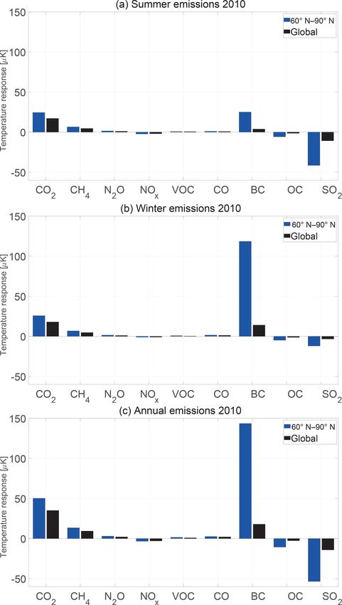
7744                                  K. J. Kupiainen et al.: Climate impact of Finnish air pollutants and greenhouse gases

(1) SLCFs refer to both cooling and warming species and in-         as well as normalized to the response of CO2 (GTP, GWP,
clude methane (CH4 ), ozone (O3 ) and aerosols (i.e., black         RTP). Especially for short-lived species, the climate impact
carbon, BC, organic carbon, OC, and sulfate) or their precur-       depends on the location and timing of the emissions, which
sors, as well as some halogenated species, and (2) SLCPs re-        is reflected in the RTPs as well as in the global response for
fer only to the warming SLCFs. Policies focusing on SLCPs           GTP and GWP. On a global scale, Unger et al. (2009) at-
have been suggested as supplements to greenhouse gas re-            tributed the RF to different economic sectors, while Aamaas
ductions (UNEP/WMO, 2011; Shindell et al., 2012, 2017;              et al. (2013) estimated the climate impact of different sectors
Rogelj et al., 2014; Stohl et al., 2015).                           based on different emission metrics for global emissions, as
   Modeling studies by UNEP/WMO (2011) and Stohl et                 well as regionally for the United States of America, China
al. (2015) suggested that the climate response of SLCF miti-        and Europe.
gation is strongest in the Arctic region. The Arctic region is         In this study we assess the climate impact of Finnish air
of particular interest, since in the past 50 years the Arctic has   pollutants – SO2 , NOx , NH3 , non-methane volatile organic
been warming twice as rapidly as the world as a whole and           compounds (NMVOCs), BC, OC and CO, and greenhouse
has experienced significant changes in ice and snow covers          gas emissions (CO2 , CH4 and N2 O) – in the past (2000–
as well as permafrost (AMAP, 2017). AMAP (2011, 2015)               2010) and until 2030, according to a baseline emission pro-
as well as Sand et al. (2016) demonstrated that emission re-        jection. We utilize emission metric values from several new
ductions of SLCFs in the northern areas have the largest tem-       studies relevant for Finland.
perature response to the Arctic climate per unit of emissions          Finnish emissions and their climate response are relatively
reduced, with the Nordic countries (Denmark, Finland, Ice-          small compared with emissions from larger regions, let alone
land, Norway and Sweden) and Russia having the largest im-          the globe. Therefore, it is challenging to use climate models
pact when compared to the other Arctic countries, the United        to study the climate effect of national policies and to analyze
States of America and Canada.                                       the role of each pollutant and sector. This study demonstrates
   Shindell et al. (2017) and Ocko et al. (2017) have argued        a method to overcome this challenge by the use of emission
for assessing both near- and long-term effects of climate           metrics. The method is applicable in other countries or re-
policy. However, comparing the climate impacts of SLCFs,            gions as well and has been used in connection with the Nor-
CO2 and other pollutants is not straightforward. Emission           wegian work on SLCPs (Norwegian Environment Agency,
metrics are one way of enabling a comparison as they pro-           2014; Hodnebrog et al., 2014).
vide a conversion rate between emissions of different species          The “Methodology” section describes the construction and
into a common unit, for example CO2 -equivalent emissions.          background data of the emission inventory and the future sce-
Common emission metrics are the global warming potential            nario as well as the emission metrics used. In the “Results”
(GWP) (IPCC, 1990) and the global temperature change po-            section we describe the emissions and their climate impacts,
tential (GTP) (Shine et al., 2005). The GWP compares the            first focusing on the historical emissions (2000–2010) and
integrated radiative forcing (RF) of a pulse emission of a          then on the future projection until 2030. We also discuss sep-
given species relative to the integrated RF of a pulse emis-        arately the regional temperature effect of emissions on the
sion of CO2 . Since the United Nations Framework Conven-            Arctic and compare the results obtained with different metric
tion on Climate Change (UNFCCC) reporting procedure uses            studies. In the “Conclusions” section we will summarize the
the GWP with a 100-year time horizon (GWP100) as a re-              main findings and draw conclusions on the major scientific
porting guideline, it has become the most common metric             and policy relevant messages.
to report greenhouse gas emissions. The GTP is an alterna-             The objectives of this study were to (1) produce an inte-
tive to GWP and it compares the temperature change at a             grated multi-pollutant emission dataset for Finland for 2000
point in time due to a pulse emission of a species relative         to 2030, (2) compare multiple climate metrics and assess
to the temperature change of a pulse emission of CO2 . The          their suitability for a northern country like Finland, (3) esti-
GTP combines the changes in the radiative forcing induced           mate the climate impact of Finnish air pollutants and green-
by the different species with the temperature response of the       house gases for the period 2000 to 2030 utilizing selected
climate system and thus has been argued to relate better to         climate metrics, and (4) suggest a set of global and regional
climate effects (Shine et al., 2005). Both GWP and GTP fo-          climate metrics to be used in connection with Finnish SLCF
cus on the global response, while the temperature impact can        emissions.
also be analyzed on a regional scale, i.e., the Arctic, applying
regional temperature change potential (RTP) (Shindell and
Faluvegi, 2010). Even for a uniform forcing, there will be          2   Methodology
spatial patterns in the temperature response. The metrics can
be presented in absolute forms of radiative forcing (absolute       Finland is one of the Nordic countries situated between lati-
global warming potential, AGWP) or temperature perturba-            tudes 60 and 70◦ N. It has a population of 5.5 million people
tion (absolute global temperature change potential, AGTP;           with an average population density of 17.9 inhabitants per
and absolute regional temperature change potential, ARTP)           square kilometer. As a comparison, the EU average is 117

Atmos. Chem. Phys., 19, 7743–7757, 2019                                              www.atmos-chem-phys.net/19/7743/2019/
K. J. Kupiainen et al.: Climate impact of Finnish air pollutants and greenhouse gases                                         7745

inhabitants per square kilometer. Although much of the pop-       2.2   Emission metrics
ulation is concentrated in the south of the country, the scarce
population compared to the country size makes transport of        This work studies Finnish emissions with several climate
goods and people an important activity. The northern loca-        metrics and focuses particularly on three of them: the AGWP
tion of the country in turn results in a high demand for en-      (IPCC, 1990), AGTP (Shine et al., 2005) and ARTP (Shindell
ergy to heat households, and the economy is largely based         and Faluvegi, 2010). AGWP at time horizon H for emissions
on energy-intensive industry.                                     of pollutant i in emission season s from emission sector t is
                                                                  defined as
2.1   Emissions
                                                                                      ZH
The historical emissions of SO2 , NOx , BC and OC in 2000,        AGWPi,s,t (H ) =         RFi,s,t (t)dt,                       (1)
2005 and 2010 are estimated based on the data in the                                  0
Finnish Regional Emission Scenario (FRES) model (Kar-
vosenoja, 2008). Emissions of NH3 , volatile organic com-         where RF is the time-varying radiative forcing given a unit
pounds (VOCs), CO2 , CH4 and N2 O are from the national           mass pulse emission at time zero. Since two recent stud-
air pollutant and greenhouse gas emission inventories as re-      ies (Aamaas et al., 2016, 2017) have separated emissions
ported to the UNFCCC and the United Nations Economic              during summer (May–October) and emissions during winter
Commission for Europe (UNECE) Convention on Long-                 (November–April), we also make this separation when pos-
Range Transboundary Air Pollution (CLRTAP). The CO                sible. AGTP is given as
emission data are estimated with the GAINS model (http:
//gains.iiasa.ac.at, last access: 13 December 2018; Amann                            ZH
et al., 2011). The data sources by pollutant are presented        AGTPi,s,t (H ) =        RFi,s,t (t)IRFT (H − t)dt.            (2)
in Table 1. Emissions of CO2 are presented according to                              0
the IPCC guidelines, which assume biomass as carbon neu-
tral. However, this definition is disputed, and, e.g., Cheru-     IRFT (H − t) is the temperature response, or impulse re-
bini et al. (2011) present emission metric values that account    sponse function for temperature, at time H to a unit radiative
for CO2 emissions from biomass. Although the historical           forcing at time t. The ARTP is similar to AGTP but gives the
emission data emanate from different data sources (Table 1),      temperature response in latitude bands m:
they have been checked for consistency and are based es-
sentially on the same statistical sources. We aggregated the                                  H
                                                                                          X Z Fl,i,s,t (t)
data and performed specific analyses for the following eight      ARTPi,m,s,t (H ) =                       × RCSi,s,l,m
major economic sectors: energy production (ENE IND), in-                                  l
                                                                                                Ei,s,t
                                                                                             0
dustrial processes (PROC), road transport (TRA RD), off-
                                                                                     × RT (H − t) dt,                           (3)
road transport and machinery (TRA OT), domestic combus-
tion (DOM), waste (WST), agriculture (AGR), and other             where Fl,i,s,t (t) is the radiative forcing in latitude band l and
(OTHER).                                                          RCSi,s,l,m is the matrix of unitless regional response coef-
   The assumptions about the future energy use, transport and     ficients based on the ARTP concept (Collins et al., 2013).
other activities in Finland follow Finland’s 2013 National        In Sand et al. (2016), RCS matrices differ for some of the
Climate and Energy Strategy (Ministry of Employment and           different sectors; for example, BC emissions in the Nordic
the Economy, 2013) and its baseline scenario that fulfills the    countries from the domestic sector have a sensitivity about
agreed EU targets and specific national targets for a share       15 % higher than BC emissions from energy and industry.
of renewables and emission reductions in the sectors outside      Aamaas et al. (2017) do not provide this information on a
the Emission Trading Scheme. Table 2 shows the primary            sector level, and we must therefore use the same RCS matrix
energy consumption by fuel in Finland in 2010 and 2030.           for all emission sectors.
The 2013 National Climate and Energy Strategy assumes the            The ARTP method divides the world into four latitude
future prevalence of wood heating to remain at 2011 levels,       bands: southern mid- to high latitudes (90–28◦ S), the trop-
which is estimated to lead to a decreased wood consump-           ics (28◦ S–28◦ N), northern midlatitudes (28–60◦ N) and the
tion, due to increasing energy efficiency in housing. The fu-     Arctic (60–90◦ N). We will focus on the temperature re-
ture emission projection was estimated with the FRES model        sponse in the Arctic, as well as the global mean response.
which used the activity estimates from the 2013 National Cli-        Some of the studies separate the net response for a pol-
mate and Energy Strategy (Table 2) as a basis.                    lutant into various processes. For the aerosols, the radia-
                                                                  tive efficiencies often include the aerosol direct and first in-
                                                                  direct (cloud-albedo) effect. In addition, BC deposition on
                                                                  snow and semi-direct effects may also be considered for BC.
                                                                  The ozone precursors build on the processes of a short-lived

www.atmos-chem-phys.net/19/7743/2019/                                              Atmos. Chem. Phys., 19, 7743–7757, 2019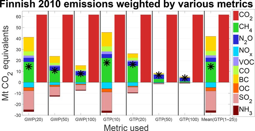
7746                                   K. J. Kupiainen et al.: Climate impact of Finnish air pollutants and greenhouse gases

Table 1. Data sources of the historical emission data for 2000–2010.

 Pollutant                                                     Data source
 Black carbon (BC), organic carbon (OC)                        FRES model
 CO                                                            GAINS model (http://gains.iiasa.ac.at, last access: 13 December 2018)
 CO2 , CH4 and N2 O from combustion sources                    FRES model
 CO2 , CH4 and N2 O from other sources than combustion         National inventory of greenhouse gases specified in the Kyoto Protocol to
                                                               the Secretary of the UNFCCC
 NH3 and VOC                                                   National emission inventory to the UNECE Convention on Long-Range
                                                               Transboundary Air Pollution (CLRTAP)

Table 2. Primary energy consumption in Finland (TWh a−1 ) (Ministry of Employment and the Economy, 2013).

                                                                           2010    2020 baseline   2030 baseline
                          Traffic fuels                                       50             48              42
                          Other oil fuels                                     48             43              32
                          Coal                                                52             50              22
                          Gas                                                 41             37              31
                          Peat                                                26             16              13
                          Wood fuels,                                         89             98             101
                          – of which residential wood combustion (RWC)        19             15              17
                          Nuclear power                                       66            106             171
                          Hydro power                                         13             14              15
                          Wind power                                         0.3              6               7
                          Others, including waste                             10             16              19
                          Import of electricity                               11              0             −3
                          Sum                                                407            433             459

ozone effect, methane effect and methane-induced ozone ef-                  The pollutants we include in our analysis (SO2 , NOx ,
fect, as well as the aerosol direct and first indirect effects.          NH3 , NMVOC, BC, OC, CO, CO2 , CH4 and N2 O) have very
   All these emission metrics (AGWP, AGTP, ARTP) can be                  different atmospheric lifetimes and impact pathways. For the
normalized to the corresponding effect of CO2 , where M is               greenhouse gases (GHGs) (CO2 , CH4 and N2 O), we use the
GWP, GTP, or RTP:                                                        climate metric parameterization in IPCC AR5 (Myhre et al.,
            AMi (t)                                                      2013), but with an upward revision of 14 % for CH4 to ac-
Mi (t) =             .                                         (4)       count for the larger radiative forcing calculated by Etminan
           AMCO2 (t)
                                                                         et al. (2016). The atmospheric decay of CO2 is parameterized
For GWP, we have included an additional analysis with the                based on the Bern Carbon Cycle Model (Joos et al., 2013) as
newly suggested metric GWP∗ (Allen et al., 2016, 2018).                  reported in Myhre et al. (2013). We assume that the relative
They argue for an alternative use of GWP to better compare               temperature response pattern in the four latitude bands is the
CO2 and SLCFs, which can be done by comparing the cu-                    same for all the GHGs, and we base our calculations on the
mulative warming of CO2 with the emission level change of                latitude pattern for CH4 in Aamaas et al. (2017).
SLCFs. For CO2 and N2 O, we have calculated GWP∗ (H )                       For all the other pollutants (SO2 , NOx , NH3 , NMVOC,
based on Eqs. (1) and (4), which leads to CO2 -equivalent                BC, OC and CO), we use several recent studies that are rele-
emissions for pollutant iL between time t1 and t2 :                      vant for the emission location, Finland (Aamaas et al., 2016,
                  t2
                  X                                                      2017; Sand et al., 2016). We have examined how metric val-
ECO2 -eq∗ ,iL =        EiL × GWPiL (H ).                       (5)       ues from all those studies can be used for Finnish emissions
                  t1                                                     and compared those, but we will mainly present combina-
For SLCFs, the CO2 -equivalent emissions are                             tions of the studies that we think combine the strengths of
                                                                         the different datasets. For a general and global view, we have
ECO2 -eq∗ ,iS = 1EiS × GWPiS (H ) × H.                         (6)       used the GWP and GTP values from Aamaas et al. (2016).
1EiS is the change in emission level for SLCP iS between                 The rest of the paper utilizes ARTP values from Aamaas
time t1 and t2 . We have compared emissions for the 2000–                et al. (2017) to estimate temperature responses, with scal-
2030 period and with a time horizon of H = 100 years.                    ing from Sand et al. (2016) for temperature responses in the

Atmos. Chem. Phys., 19, 7743–7757, 2019                                                   www.atmos-chem-phys.net/19/7743/2019/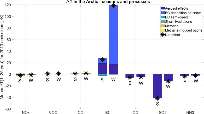
K. J. Kupiainen et al.: Climate impact of Finnish air pollutants and greenhouse gases                                        7747

Arctic. Aamaas et al. (2017) is our starting point as this study    taking the area-weighted global mean based on the results for
has the full set of emissions and separates summer and winter       the latitude bands. As the forcing-response coefficients are
emissions.                                                          different and the ARTP concept can better parameterize vary-
   No studies have presented climate metric values specific         ing efficacies, the estimated global temperature response may
to Finnish emissions. The default choice would be to use cli-       vary depending on whether it is based on AGTPs or based on
mate metric values based on global emissions, while we be-          ARTPs.
lieve using smaller emission regions near or including Fin-            Our climate impact dataset can be analyzed in many differ-
land is more representative than applying the global average.       ent dimensions, such as for different timescales, for different
The most relevant emission regions in the three selected stud-      emission sectors, for different processes, or for pulse or sce-
ies are Europe (consisting of western Europe, eastern mem-          nario emissions. We show some examples. As we focus on
bers of the European Union and Turkey, up to 66◦ N) for Aa-         near-term climate change and the global and regional tem-
maas et al. (2016, 2017) and the Nordic countries for Sand          perature, most of the discussion in this paper utilizes ARTP
et al. (2016). The Nordic countries is a smaller region and         for the mean warming in the first 25 years after a pulse emis-
is geographically more representative of Finland than Eu-           sion, as recently proposed by Shindell et al. (2017). Mean
rope is. Therefore, we have calculated ratios between met-          ARTP (1–25 years) is the average temperature response over
rics for the Nordic region vs. Europe in Sand et al. (2016)         the time period, which differs from ARTP (25 years), being
and used those ratios to scale the metric values from Aamaas        a snapshot at the time horizon of 25 years. It has similarities
et al. (2017) to better represent Finnish emissions. However,       to the integrated global temperature change potential (iGTP)
Sand et al. (2016) provided climate metric values only for          concept introduced by Peters et al. (2011). We want to point
the Arctic response, their set of pollutants was limited to         out that our choice of metric is not based on a thorough sci-
BC, OC and SO2 , and for the ozone precursors they included         entific analysis but rather is a subjective choice to study the
only a combined response. To solve this we have used av-            near-term climate impacts and the importance of short-lived
erages, such as taking a weighted average of the different          species in more detail. To balance the choice we compare it
emission sectors for each pollutant and assuming that NH3           with some other known climate metrics.
can be scaled by an average of BC, OC and SO2 . The scaling
we have done for the Arctic responses is 2.22 for BC, 3.09
for BC deposition in snow, 2.32 for OC, 1.94 for SO2 , 2.16         3     Results
for NH3 , and 1.00 for NOx , CO and NMVOC. This scaling
for the Arctic will also increase the global responses but will     3.1    Emissions
not affect the coefficients for the other temperature response
bands.                                                              Figure 1 shows the Finnish emissions and their trends from
   For all the pollutants, the IRF for temperature comes from       2000 until 2030 for the studied pollutants. Emissions by sec-
the Hadley Centre Coupled Model version 3 (HadCM3)                  tor for 2000, 2010 and 2030 can be found in Table S1 of
(Boucher and Reddy, 2008). Hence, our temperature calcu-            the Supplement. Emission reductions are expected for prac-
lations are based on a climate sensitivity of 3.9 K warming         tically all of the pollutants and greenhouse gases, especially
for a doubling in CO2 concentration.                                between 2010 and 2030, but the magnitude differs between
   Most emissions stay relatively constant throughout the           the species. Reductions of CO2 and SO2 take place to a large
year, while the changing seasons result in much larger emis-        extent in the energy production sector following the reduc-
sions from the domestic sector in winter than in summer. We         tion of energy consumption of fossil fuels, i.e., coal, oil and
account for this seasonality for those metric datasets compat-      peat (Table 2).
ible with this; otherwise, annual emission and metric values            CH4 emissions have declined mostly due to developments
are applied.                                                        in the waste sector. The amounts of methane recovered from
   The global and regional temperature responses of Finnish         landfills have increased during the study period following EU
emissions are estimated by convolving ARTP values with              and national regulations. Methane emissions from landfills
emissions. For an emission scenario E(t), the global tem-           have also declined because there has been an increase in the
perature response is                                                use of municipal solid waste for energy instead of depositing
                Zt                                                  it in landfill, a development that is expected to continue also
                                                                    until 2030. Another factor explaining the declining emissions
                     Ei,s,t (t 0 ) × AGTPi,s,t t − t 0 dt 0

1Ti,s,t (t) =                                                 (7)
                                                                    by 2030 is the prohibition of the disposal of organic waste to
                0                                                   landfills after 2016.
based on AGTP values. Similarly, the temperature responses              The transport sector is responsible for the decline in the
in latitude bands can be estimated by replacing AGTP with           emissions of CO, NOx and VOC as well as the particle
ARTP values. As mentioned, the ARTP method divides the              species, BC and OC. The modernization of vehicles and con-
world into four latitude bands, and thus the global tempera-        sequent introduction of stricter emission controls required by
ture response can also be estimated by using the ARTPs and          the European emission standards explain the decline in CO,

www.atmos-chem-phys.net/19/7743/2019/                                                  Atmos. Chem. Phys., 19, 7743–7757, 2019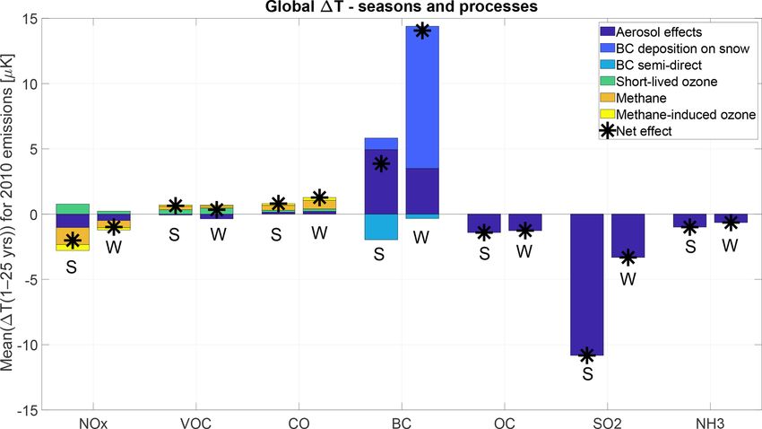
7748                                  K. J. Kupiainen et al.: Climate impact of Finnish air pollutants and greenhouse gases

                                                                     Figure 2. Finnish 2010 emission (Mt CO2 equivalents) as a pulse
                                                                     emission weighted by various global metrics. CO2 is separated out
                                                                     and the net impact of the non-CO2 is given by the star.

Figure 1. Finnish emissions (Gg a−1 ) of air pollutants and green-
house gases in the period 2000 to 2030 in the baseline scenario.     of the warming effect of CO2 , but overall the net impact of
Emissions by sector for 2000, 2010 and 2030 can be found in Ta-      all short-lived species is about 30 % of CO2 , due to the partly
ble S1 of the Supplement.                                            counteracting cooling effect of NH3 , SO2 , NOx and OC. The
                                                                     relative importance of the SLCFs decreases with time, espe-
                                                                     cially with GTP, as expected, and the relative effect is lowest
NOx and NMVOC emissions. The standards do not directly               with the temperature change metric with 100-year time hori-
regulate BC or OC emissions, but since they are the main             zon (GTP100), being about 6 % of CO2 . Among the non-CO2
constituents of the regulated particulate emissions, reduc-          emissions, the relative impact of N2 O increases with increas-
tions in emissions of BC and OC are expected, especially af-         ing time horizon due to the much longer atmospheric lifetime
ter the introduction of the diesel particulate filters for on-road   than for the other pollutants.
light-duty vehicles from 2010 onwards. The heating stoves               An alternative to comparing emissions pulses with GWPs
and boilers in the residential sector will remain significant        and GTPs is to consider the impact over a particular emission
emitters of several pollutants, since the regulation follow-         time period with GWP∗ (Allen et al., 2016, 2018). Figure 3
ing the European Union Ecodesign directive will not have             presents a GWP∗ -based analysis of Finnish emissions. As we
a major impact by 2030, due to the relatively long lifetime of       have looked at emissions for the period 2000–2030, the CO2 -
Finnish heaters (Savolahti et al., 2016).                            equivalent emissions given in Fig. 3 are not directly compa-
   NH3 and N2 O emissions remain relatively stable through-          rable to those based on pulses in Fig. 2. We find that changes
out the study period, since either much of the emission re-          in global temperature in this period are mostly governed by
ductions has already taken place before the study period or          the cumulative emissions of CO2 . The emissions of multi-
no major changes are expected in the main emission sectors           ple SLCFs decline in this period (Fig. 1), resulting in a net
(agriculture for NH3 ).                                              cooling and counteracting 4 % of the warming by CO2 and
                                                                     N2 O. If emissions of all SLCFs were hypothetically reduced
3.2    Climate impact of Finnish emissions                           to zero in this period, this emission change could counteract
                                                                     the warming by CO2 and N2 O by about one-third. Similarly,
Figure 2 shows pulses of 2010 emissions weighted with the            as for GWPs and GTPs (Fig. 2), we find that emission of CO2
global metrics (GWP and GTP) to CO2 equivalents using 10-            has the largest impact of all pollutants.
, 20-, 50- and 100-year perspectives. Aamaas et al. (2013)              As we focus on near-term climate change and the global
studied global emissions with these metrics, while we focus          and regional temperature, the remaining paper utilizes ARTP
in detail on Finnish emissions. In addition, we show the emis-       with a time horizon of mean GTP (1–25 years), as proposed
sion metric mean GTP (1–25 years), which gives the SLCFs             by Shindell et al. (2017). ARTP values are applied, follow-
a relatively large weight, similar to GTP (10 years) for the         ing the argumentation by Aamaas et al. (2017) that ARTPs
aerosols and in between GTP (10 years) and GTP (20 years)            may give a better estimate of the global impact than AGTPs
for CH4 . In Fig. 2 the emissions are considered as a pulse          since they account for varying efficacies with latitude to a
and the figure does not take into account any emissions af-          larger degree. The ARTP (1–25 years) used in this study is
ter 2010. Figure 2 demonstrates that the SLCFs have a larger         presented in Table 3. GWP∗ could also be a basis to esti-
relative importance with the metrics for shorter time hori-          mate global temperature changes, but that would not give us
zons. However, in all cases CO2 still is the most important          regional temperature changes.
species. With the emission metric with the 10-year horizon
(GTP10) the warming SLCFs comprise more than two-thirds

Atmos. Chem. Phys., 19, 7743–7757, 2019                                               www.atmos-chem-phys.net/19/7743/2019/
K. J. Kupiainen et al.: Climate impact of Finnish air pollutants and greenhouse gases 7749
Table 3. The climate metric values (◦ C Tg−1 ) used in this study. Mean ARTP (1–25 years) values for SLCF and GHG emissions. The Arctic
response for the GHGs is based on the latitudinal pattern for CH4 . The annual average is based on emissions in 2010. Normalized values
(CO2 equivalents) are shown in Table S2.
Mean (1–25 years), global response in ◦ C Tg−1 Mean (1–25 years), Arctic response in ◦ C Tg−1
Annual average Summer Winter Annual average Summer Winter
CO2 [CO2 ] 5.7 × 10⁻⁷ 5.7 × 10⁻⁷ 5.7 × 10⁻⁷ 8.2 × 10⁻⁷ 8.2 × 10⁻⁷ 8.2 × 10⁻⁷
CH4 [CH4 ] 4.8 × 10⁻⁵ 4.8 × 10⁻⁵ 4.8 × 10⁻⁵ 6.9 × 10⁻⁵ 6.9 × 10⁻⁵ 6.9 × 10⁻⁵
N2 O [N2 O] 1.5 × 10⁻⁴ 1.5 × 10⁻⁴ 1.5 × 10⁻⁴ 2.1 × 10⁻⁴ 2.1 × 10⁻⁴ 2.1 × 10⁻⁴
NOx [NO2 ] −1.7 × 10⁻⁵ −2.3 × 10⁻⁵ −1.1 × 10⁻⁵ −1.9 × 10⁻⁵ −2.7 × 10⁻⁵ −1.1 × 10⁻⁵
VOC [VOC] 9.6 × 10⁻⁶ 1.4 × 10⁻⁵ 6.1 × 10⁻⁶ 1.6 × 10⁻⁵ 1.6 × 10⁻⁵ 1.6 × 10⁻⁵
CO [CO] 4.1 × 10⁻⁶ 3.9 × 10⁻⁶ 4.3 × 10⁻⁶ 5.2 × 10⁻⁶ 5.0 × 10⁻⁶ 5.4 × 10⁻⁶
BC [C] 2.7 × 10⁻³ 1.5 × 10⁻³ 3.4 × 10⁻³ 2.2 × 10⁻² 1.0 × 10⁻² 2.9 × 10⁻²
OC [C] −4.7 × 10⁻⁴ −6.7 × 10⁻⁴ −3.5 × 10⁻⁴ −1.9 × 10⁻³ −2.7 × 10⁻³ −1.4 × 10⁻³
SO2 [SO2 ] −2.2 × 10⁻⁴ −3.5 × 10⁻⁴ −1.0 × 10⁻⁴ −8.5 × 10⁻⁴ −1.3 × 10⁻³ −3.7 × 10⁻⁴
NH3 [NH3 ] −4.3 × 10⁻⁵ −5.2 × 10⁻⁵ −3.3 × 10⁻⁵ −1.4 × 10⁻⁴ −1.7 × 10⁻⁴ −1.1 × 10⁻⁴
the domestic sector, and since this study considers wood fuel
as CO2 neutral, the CO2 warming effect is not as pronounced
as, for example, in the on-road transport sector. Organic car-
bon was the most important cooling agent in domestic and
the transport sectors, as fuelwood does not contain much sul-
fur. Furthermore, it was phased out from liquid fuels in the
transport sector. Overall, SO2 is the major cooling pollutant
mainly due to emissions from ENE IND and PROC. Agricul-
ture is an important source of ammonia (NH3 ), which has a
cooling effect (Figs. 4a–c and 5a) via its participation in the
formation of cooling atmospheric aerosols like ammonium
Figure 3. The CO2 -equivalent emissions for the period 2000–2030 sulfates and nitrates.
given the alternative metric GWP∗ (100). The net impact of SLCFs The year 2000 was relatively warm and 2010 relatively
(left) and CO2 and N2 O (right) is given by the star. cold in Finland, which is reflected by the higher use of coal,
peat and wood fuels in 2010 and consequently also by the
higher emissions of some species. From 2000 to 2010, CO2
3.2.1 Climate impacts by emission sector emissions from ENE IND increased by 22 % and BC emis-
sions from DOM by 37 %. However, because of additional
This section discusses the global temperature response of mitigation measures following legislation, CH4 emissions
the emissions by pollutant and emission sector based on from the WST decreased by 38 %. Also, despite the higher
weighted ARTP values (Aamaas et al., 2017). The general fuel use, improved flue gas cleaning measures caused SO2
findings described in the following paragraphs would be sim- emissions in ENE IND to decrease by 18 %. On the other
ilar with AGTPs, and similar figures based on the AGTP val- hand, the reduction of SO2 increased the warming effect of
ues (Aamaas et al., 2016) can be found in Fig. S1 of the Sup- the ENE IND sector in 2010 compared to 2000. The increas-
plement for comparison. Figure 4a, b and c show the warm- ing SLCF emissions in the DOM sector, particularly black
ing due to emissions in 2000, in 2010 and in 2030, following carbon, led to additional net warming despite the fact that
the baseline projection, respectively. The sum of all sectors the organic carbon emissions offset about a fifth of the black
is given in Fig. 4d. The pollutant mix varies for the different carbon effect in both years. The decreasing trend for the use
sectors. CO2 is the most important pollutant for combustion of heating oil in the domestic sector has reduced CO2 emis-
in ENE IND and TRA RD, while methane is most impor- sions between 2000 and 2010. Emissions from the PROC
tant for the WST and AGR sectors. BC emissions cause more sector are relatively neutral in terms of their climate effect. In
than two-thirds of the warming, increasing over time in DOM general, taking into account all sectors, the emission changes
and causing a significant share of the warming in TRA RD as between 2000 and 2010 in Finland have led to net warming
well as TRA OT sources. The rest of the warming effect for (increase by 7 %), mostly due to the increase in CO2 emis-
these sectors is due to CO2 emissions from fossil fuels, espe- sions (warming) and the decrease in SO2 emissions (warm-
cially diesel and light fuel oil. Wood is an important fuel in
www.atmos-chem-phys.net/19/7743/2019/ Atmos. Chem. Phys., 19, 7743–7757, 20197750 K. J. Kupiainen et al.: Climate impact of Finnish air pollutants and greenhouse gases
Figure 4. The temperature response (µK) due to emissions in 2000 (a), 2010 (b) and 2030 (c) from energy and industry sectors (ENE
IND), industrial processes (PROC), road transport (TRA RD), off-road transport and machinery (TRA OT), domestic (DOM), waste (WST),
agriculture (AGR) and other (OTHER). The sum of all sectors is shown in (d). The climate metric applied is the global mean ARTP (1–25
years) for pulse emissions.
ing) from the ENE IND sector, which offset the reduction of methane emissions in the WST sector continue their decline
CH4 emissions (cooling) in the WST sector. (Fig. 4b and c). As a consequence of the emission changes,
The baseline projection will lead to an emission reduction the net temperature impact of 2030 emissions is 35 % lower
of all pollutants between 2010 and 2030, from a reduction of compared to the 2010 emissions (Fig. 4d). Practically all sec-
BC greater than 50 % to a small reduction of N2 O (Fig. 1 and tors except AGR contribute to the reduced warming (Fig. 4b,
Table S1). Because of climate policies, CO2 emissions are c).
reduced following the declining use of fossil fuels (Table 2,
Fig. 4b, c and d). The SO2 emissions continue their decline 3.2.2 Cumulative temperature development 2000–2030
between 2010 and 2030, particularly in the ENE IND sec-
tor, which leads to additional warming but only partly off- While most of our study focuses on emission pulses, in this
sets the reduced CO2 (Fig. 4b, c and d). In the TRA RD section we will discuss global temperature responses given a
and TRA OT sectors, the warming effect from the SLCFs, convolution of a Finnish emission scenario and ARTP values.
in particular, declines because the new vehicles, in order to The cumulative global temperature impact by pollutants and
comply with the European emission legislation, are equipped sectors for Finnish emission from 2000 to 2030 is shown in
with efficient emission reduction technologies (Fig. 4b and Fig. 5, based on ARTPs in Aamaas et al. (2017) and Sand
c). The amount of domestic wood combustion is expected to et al. (2016). Similar figures based on AGTP values (Aa-
decrease in the baseline due to improved energy efficiency maas et al., 2016) are given in Fig. S2 of the Supplement.
in housing, which is the main reason for the reduced SLCF Figure 5 demonstrates why emission reductions of CO2 and
emissions in the sector (Fig. 4b and c). However, when in- other long-lived greenhouse gases are key for limiting the
terpreting these results, it is important to note that the preva- long-term surface temperature increase. As more years are
lence of domestic wood combustion has increased during the added, the relative importance of CO2 increases, since a large
2000s and the future wood use in households is challenging portion of it stays in the atmosphere for hundreds of years.
to predict. Therefore, the emissions from the domestic sec- This relative importance over time also occurs in the case of
tor should be considered uncertain. This is demonstrated in a N2 O. The air pollutants become of less relative significance
sensitivity analysis of future particle emissions from the do- with time, which is mostly because of those pollutants being
mestic sector presented by Savolahti et al. (2016). Also, the quickly removed from the atmosphere, but also because of
the reduced emissions levels in the later period. Almost all
Atmos. Chem. Phys., 19, 7743–7757, 2019 www.atmos-chem-phys.net/19/7743/2019/K. J. Kupiainen et al.: Climate impact of Finnish air pollutants and greenhouse gases 7751
Figure 6. The global temperature response (µK) of Finnish emis-
sions in 2010 by applying the mean temperature 1–25 years after
the pulse emission. This figure compares emissions occurring in
summer (S) vs. winter (W) by applying ARTP values (Aamaas et
al., 2017; Sand et al., 2016). The responses are divided into six dif-
ferent processes.
and NOx . The same process can be warming for one pol-
lutant and cooling for another; for example NOx emissions
remove CH4 from the atmosphere (cooling), while VOC and
Figure 5. The global temperature development (mK) of Finnish CO emissions add CH4 (warming). Changes in the methane
emissions for the period 2000–2030. Temperature is given by pol-
concentration will also influence ozone, giving rise to the
lutants in (a) and by sectors in (b). The global temperatures are es-
timated as a convolution of ARTP values and an emission scenario.
methane-induced ozone effect and reinforcing the methane
effect.
For 1 t of BC emission with the ARTP metric, the winter-
time impact is higher by more than 120 % than the summer-
sectors have a net warming temperature response, with the
time impact. Almost 80 % of the net impact for winter emis-
exception of cooling from the ENE IND sector for more than
sion comes for BC deposition on snow. The annual impact
the first 10 years and a slight cooling from the PROC sec-
of winter emissions of BC is almost 80 % with the ARTPs.
tor until 2030 (Fig. 5b). Cooling from mainly SO2 emissions
From a mitigation perspective, these estimates indicate that
offsets the warming impact of CO2 from those sectors. Over
attention should be placed on reducing winter emissions of
time, ENE IND becomes the most influential sector, being
BC.
the single largest contributor of CO2 . BC is the most signif-
icant warming pollutant in the domestic sector, and in the 3.2.4 Arctic temperature response from Finnish
agriculture and waste sectors, it is CH4 . emissions
3.2.3 Seasonal temperature response from Finnish The seasonal differences for the SLCFs are also clearly seen
emissions in the Arctic temperature response (Fig. 7). Finland is closely
situated to the Arctic as practically the whole country is north
The estimated temperature response of Finnish emissions of 60◦ N and a significant area lies north of the Arctic Circle.
varies between the seasons. In Fig. 6, we compare Finnish Figure 7 shows the Arctic (between 60 to 90◦ N) tempera-
SLCF emissions for the year 2010 during summer (May– ture response based on the ARTP metrics from Aamaas et
October) and winter (November–April). A decomposition al. (2017) and Sand et al. (2016). As a general observation,
into different atmospheric forcing processes is also included. the temperature responses are larger in the Arctic (Fig. 7)
When we do not consider CO2 , N2 O and CH4 , the pollutants than globally (Fig. 6). The trends are similar, with net cooling
give a net cooling for emissions in summer and a net warm- of summer emissions and net warming of winter emissions.
ing of equal size for emissions in winter. The main driver for The Arctic warming in winter is up to about 3 times larger
this is larger BC emissions in winter combined with a much than the cooling in summer, mostly due to the outsized im-
stronger response from the snow albedo effect. The reason pact of wintertime emissions of BC. However, during sum-
is that more than 70 % of the annual emissions in the do- mer, the cooling by SO2 emissions outweighs the warming
mestic sector occur in winter. Another important difference by BC emissions.
is the much stronger cooling by SO2 in summer. Some pollu-
tants have both warming and cooling processes, such as BC
www.atmos-chem-phys.net/19/7743/2019/ Atmos. Chem. Phys., 19, 7743–7757, 20197752 K. J. Kupiainen et al.: Climate impact of Finnish air pollutants and greenhouse gases
Figure 7. The temperature response (µK) in the Arctic of Finnish
emissions in 2010, by applying the mean temperature 1–25 years
after the pulse emission. This figure compares emissions occurring
in summer (S) vs. winter (W) by applying ARTP values (Aamaas et
al., 2017; Sand et al., 2016).
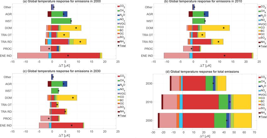
Figure 8 compares global and Arctic temperature re-
sponses to Finnish emissions of all pollutants considered
in this study, using the Aamaas et al. (2017) approach. It
demonstrates that the temperature response in the Arctic is
typically stronger than the global average. If we apply the
ARTP methodology for GHGs, the response in the Arctic is
up to 50 % larger than the global average due to stronger lo-
cal feedback processes in the Arctic (Boer and Yu, 2003).
The ozone precursors have similar or weaker efficacies in
the Arctic compared with the GHGs. However, the aerosols
and sulfur emissions stand out with the largest differences
(Fig. 8). By applying ARTP values from Aamaas et al. (2017)
with scaling from Sand et al. (2016), we find that Finnish
emissions of SO2 and OC have a 300 % stronger efficacy in
the Arctic than the global average, and this is even higher for
BC with 700 %. A limitation of this method is that the scal-
ing from Sand et al. (2016) is only applicable for the Arctic
temperature response, which adds some uncertainties to the Figure 8. Global and Arctic (60–90◦ N) temperature responses (µK)
Arctic vs. global ratios. For BC, this amplification in the Arc- to Finnish emissions based on ARTP values in Aamaas et al. (2017)
tic is even stronger for emissions occurring in winter. Hence, and Sand et al. (2016). As for most of the figures, the temperature
the results indicate that mitigation of Finnish BC emissions response is the mean response 1 to 25 years after a pulse emission.
is especially beneficial for limiting Arctic warming.
4 Discussion Our second set of objectives for this study aimed to com-
pare different climate metrics and to assess their suitability
The first objective in our study was to produce an inte- for calculating the climate impact of a multi-pollutant emis-
grated multi-pollutant emission dataset for Finland for 2000 sion set. Several air pollutants and greenhouse gases have
to 2030. We were able to achieve this aim, but it required detrimental impacts on global and regional climate, human
the use of several data sources and studies that are not nec- health and wellbeing, as well as crop yields (Shindell et al.,
essarily maintained on a regular basis. Future efforts should 2012). Since the magnitudes and pathways of the effects dif-
seek to maintain the integrated multi-pollutant database de- fer between the constituents, integrated modeling is needed
veloped for this work. This would require an integrated mod- to understand the consequences and form the basis for ro-
eling environment, for example the FRES, and would require bust climate and air quality policies. This paper applied and
further work to fill in the gaps for the missing sectors and pol- compared various climate metrics to study the approximate
lutants via developing relevant activity and emission factor integrated climate impact of Finnish air pollutant and green-
databases into the FRES framework. house gas emissions globally and in the Arctic area. The re-
Atmos. Chem. Phys., 19, 7743–7757, 2019 www.atmos-chem-phys.net/19/7743/2019/K. J. Kupiainen et al.: Climate impact of Finnish air pollutants and greenhouse gases 7753 sults demonstrated that the relative impacts and importance warming impact, and although that is expected to decrease of individual species as well as sectors can differ significantly notably by 2030 due to stricter control on particulate and between the studied temporal-response scales, emission sea- black carbon emissions, it will remain a major source of car- sons as well as geographical scales for both emission sources bon dioxide. Emissions from domestic and agriculture sec- and temperature responses. The warming or cooling impact tors also have a considerable warming impact, and they will of SLCFs is especially sensitive to the studied timescale, remain as such, due to the relatively large respective emis- with shorter time spans showing greater importance com- sions of black carbon and methane from the combustion of pared with GHGs. solid fuels, especially wood. Finnish emissions and their climate responses are rela- For all of the species the temperature response of Finnish tively small; therefore, it is challenging to use climate models emissions is generally stronger in the Arctic than globally to study the climate effect of national policies and to analyze but most significantly so in the case of black carbon and sul- the role of each pollutant and sector. This study demonstrated fur dioxide. Results obtained with the ARTP metric indicated a method to overcome this challenge by utilizing emission that mitigation of wintertime black carbon emissions is espe- metrics. All studied metrics provided interesting insights into cially important for reducing the temperature increase in the the impacts of Finnish emissions and which aspects could Arctic. Emissions of sulfur dioxide are expected to continue be emphasized when formulating mitigation strategies. We decreasing, and this has many benefits (Ekholm et al., 2014). found that the ARTP-based metrics, in particular, provided However, they will offset some of the climate benefits of the useful information. We preferred to use ARTP approaches to reduced carbon dioxide emissions, and this should be taken assess the impacts of Finnish emissions on both the global into consideration in climate assessments. and Arctic climates because they include the regional or lat- The fourth major objective of this study was to recommend itudinal dimension of emission impacts in more detail. We a set of global and regional climate metrics to be used in also chose to use the mean 1–25-year time frame, since for connection with Finnish SLCF emissions. As a preparation the time being there are no established climate metrics for for writing this paper we compared several climate metrics air pollutants, and this approach was recently suggested by to be used in connection with Finnish SLCF emissions. We Shindell et al. (2017) to be used in connection with SLCFs. ended up relying on those presented in Aamaas et al. (2017), This is a subjective choice to study the near-term climate im- which to our understanding, is currently the most complete pacts and the importance of short-lived species in more de- set of climate metrics available for assessing the global and tail. To our knowledge, we are the first to present metric val- Arctic temperature responses of European emissions. How- ues with mean ARTP (1–25 years) and among the first to use ever, we have scaled those values with ratios from Sand et the GWP∗ . al. (2016) for the Arctic temperature response because that The use of ARTPs to study the impacts of Finnish emis- study provided ARTPs for Nordic emissions, which are more sions is useful for designing national emission mitigation representative of the Finnish case. For the GHGs, we ar- strategies also from a regional perspective. Finland is an Arc- gue for the application of the metric parameterization from tic country and a member of the Arctic Council, which is why IPCC AR5 (Myhre et al., 2013) but with an upward revision there is high interest in understanding the Arctic impacts. for CH4 (Etminan et al., 2016). The coefficients for mean The third set of objectives aimed to estimate the climate ARTP (1–25 years) (see also Shindell et al., 2017) in Ta- impact of Finnish air pollutants and greenhouse gases uti- ble 3 were used for assessing different mitigation pathways lizing the selected metrics. Our analysis across climate met- in a 25-year time span. This time window is relevant for poli- rics, time horizons, pollutants and Finnish emission path- cies that focus on reducing global or Arctic warming in the ways demonstrated that carbon dioxide emissions have the near or medium term, from today and until 2040 or 2050. largest climate response also in the near term (10 to 20 years), Corresponding mean RTP (1–25 years) values are shown in and their relative importance increases the longer the time Table S2. span gets. Hence, mitigation of carbon dioxide is crucial The assessed temperature impact of an emission dataset for reducing the climate impact of Finnish emissions. In the depends on the set of metrics available, as well as the ap- near or medium term (i.e., 25-year perspective), methane and plied metric setup, which bring uncertainties to the results. black carbon, in particular, have relatively significant warm- As there is no consensus on one individual set of metrics, ing impacts in addition to those of carbon dioxide. SO2 , on especially in the case of air pollutants, the results will differ the other hand, is an important precursor to light-reflecting between different studies. This work estimated the global and sulfate aerosol, thus having a cooling impact and offsetting regional temperature impacts of Finnish emissions based on part of the warming impact of the other species. methodologies in three recent papers (Sand et al., 2016; Aa- Concerning Finnish emissions, the combustion in energy maas et al., 2016, 2017). As all of these studies utilize partly production and industry has the largest global temperature the same radiative forcing datasets and partly similar gen- impact over the medium and long term due to significant eral circulation models and chemistry transport models, we carbon dioxide emissions, while sulfur dioxide emissions in- welcome other studies to complement the basis of our find- duce a shorter-term cooling. Transport has the second biggest www.atmos-chem-phys.net/19/7743/2019/ Atmos. Chem. Phys., 19, 7743–7757, 2019
7754                                  K. J. Kupiainen et al.: Climate impact of Finnish air pollutants and greenhouse gases

ings. Future work should continue to explore uncertainties           5   Conclusions
and provide improved metrics.
   Since the atmospheric lifetime of SLCFs is relatively             All studied metrics provided interesting insights into the im-
short, their climate impact is more dependent on the emission        pacts of Finnish emissions and which aspects could be em-
region than with GHGs. Using Europe and the Nordic region            phasized when formulating mitigation strategies. We found
as proxies for the emission region, as in this study, gives          that particularly the ARTP-based metrics provided useful in-
us a more representative picture of the Finnish case than            formation, although one should not rule out the significance
the global average would give. Further development of the            of the other temperature and radiative-forcing-based metrics
metrics should use more precisely the geographical location          due to their relevance in connection with climate change mit-
of Finland as the emission region in order to provide more           igation work of the UNFCCC and IPCC. In the future, other
precise temperature estimates for the Finnish emissions. The         climate impact metrics should also be explored and utilized.
snow albedo effect of BC is expected to be much larger for           To enable such policy analyses an integrated multi-pollutant
the northernmost emissions, as indicated by a study on Nor-          emission and metrics database, similar to the one used in this
way by Hodnebrog et al. (2014). Future work should also fo-          work, should be maintained.
cus on providing metrics for potentially missing species that           Our analysis across climate metrics, time horizons, pollu-
could be important, for example dust aerosol.                        tants and Finnish emission pathways demonstrated that car-
   Scientific literature has demonstrated that the climate im-       bon dioxide emissions have the largest climate response also
pact of biomass combustion may depend on the timescale               in the near-term, 10- to 20-year time perspective, and its
and forestry practices (i.e., Cherubini et al., 2011; Repo et al.,   relative importance increases the longer the time span gets.
2012, 2015), which have not been a focus of this study. Since        Hence, mitigation of carbon dioxide is crucial for reduc-
the use of biomass for energy is important in Finland and            ing the climate impact of Finnish emissions. In the near or
will likely remain so in the coming decades, future studies          medium term (i.e., 25-year perspective), methane and black
could utilize metrics to study its climate impacts. This study       carbon, in particular, have relatively significant warming im-
has mostly focused on surface temperature metrics; however,          pacts additional to those of carbon dioxide.
other interesting impacts could be studied using the metric             For all of the species the temperature response of Finnish
approach. For example Shine et al. (2015) has recently pre-          emissions is generally stronger in the Arctic than globally,
sented a new metric named the global precipitation change            but most significantly so in the case of black carbon and sul-
potential (GPP), which is designed to gauge the effect of            fur dioxide. The wintertime emissions, in particular, are net
emissions on the global water cycle.                                 warming, and even more so in the Arctic, mostly due to black
   The understanding of the impact pathways of different pol-        carbon. The snow albedo effect of the Finnish BC emissions
lutants has improved in recent years, which has led to further       is found to be large, and this phenomenon should be ade-
revisions of the climate impact estimates. Such developments         quately included in the analyses. Since the atmospheric life-
are expected to continue. The metric studies, however, are of-       time of SLCFs is relatively short, their climate impact is more
ten based on earlier radiative forcing studies, and there is a       dependent on the emission region than with GHGs. Using the
time lag between new scientific understanding and this being         Finnish case, our study demonstrated that future studies and
reflected in the climate metrics. This study has utilized the        further development of the metrics should use precisely the
latest metric studies, but there is already literature available,    geographical location as the emission region in order to pro-
for instance on BC, indicating that the temperature response         vide more precise temperature estimates.
may be smaller than demonstrated by the metrics used in this
work (e.g., Stjern et al., 2017). As the understanding of the
climate system improves, the estimates we give here for Fin-
land should be revisited.

Atmos. Chem. Phys., 19, 7743–7757, 2019                                               www.atmos-chem-phys.net/19/7743/2019/
K. J. Kupiainen et al.: Climate impact of Finnish air pollutants and greenhouse gases                                                  7755

Data availability. The emission input data and metric values used       from multiple models, Atmos. Chem. Phys., 17, 10795–10809,
and produced in this study are available in Table 3, the Supplement     https://doi.org/10.5194/acp-17-10795-2017, 2017.
and in the citations. The numerical output datasets can be accessed   Allen, M. R., Fuglestvedt, J. S., Shine K. P., Reisinger, A.,
without any restrictions by contacting the corresponding author.        Pierrehumbert, R. T., and Forster, P. M.: New use of
                                                                        global warming potentials to compare cumulative and short-
                                                                        lived climate pollutants, Nat. Clim. Change, 6, 773–776,
Supplement. The supplement related to this article is available         https://doi.org/10.1038/nclimate2998, 2016.
online at: https://doi.org/10.5194/acp-19-7743-2019-supplement.       Allen, M. R., Shine K. P., Fuglestvedt, J. S., Millar, R. J., Cain, M.,
                                                                        Frame, D. J., and Macey, A. H.: A solution to the misrepresenta-
                                                                        tions of CO2 -equivalent emissions of short-lived climate pollu-
Author contributions. KJK and MS compiled the emission data             tants under ambitious mitigation, Climate and Atmospheric Sci-
with supporting contributions from NK and VVP. BA prepared the          ence, 1, 16, https://doi.org/10.1038/s41612-018-0026-8, 2018.
climate metrics databases and applied them to the emission data.      Amann, M., Bertok, I., Borken-Kleefeld, J., Cofala, J., Heyes,
KJK, BA and MS led the preparation of the paper. NK and VVP             C., Höglund-Isaksson, L., Klimont, Z., Nguyen, B., Posch, M.,
acted as contributing authors.                                          Rafaj, P., Sandler, R., Schöpp, W., Wagner, F., and Winiwarter,
                                                                        W.: Cost-effective control of air quality and greenhouse gases
                                                                        in Europe: Modeling and policy applications, Environ. Modell.
                                                                        Softw., 26, 1489–1501, 2011.
Competing interests. The authors declare that they have no conflict
                                                                      AMAP (Quinn, P. K., Stohl, A., Arneth, A., Berntsen, T., Burkhart,
of interest.
                                                                        J. F., Christensen, J., Flanner, M., Kupiainen, K., Lihavainen, H.,
                                                                        Shepherd, M., Shevchenko, V., Skov, H., and Vestreng, V.): The
                                                                        Impact of Black Carbon on Arctic Climate, Arctic Monitoring
Acknowledgements. This study has been financially supported by          and Assessment Programme (AMAP), Oslo, 128 pp., ISBN 978-
the Finnish Ministry of the Environment and the Ministry for For-       82-7971-069-1, 2011.
eign Affairs of Finland via the Baltic Sea, Barents and Arctic re-    AMAP: Black Carbon and Ozone as Arctic Climate Forcers, Arc-
gion co-operation program and by the Academy of Finland project         tic Monitoring and Assessment Programme (AMAP), Oslo, Nor-
grants, as well as by NordForsk under the Nordic Program on             way, vii + 116 pp., ISBN 978-82-7971-092-9, 2015.
Health and Welfare. Borgar Aamaas has been funded by the Eu-          AMAP: Snow, Water, Ice and Permafrost in the Arctic (SWIPA),
ropean Union Seventh Framework Programme.                               Arctic Monitoring and Assessment Programme (AMAP), Oslo,
   The authors would like to thank the editor and the referees for      Norway, xiv + 269 pp., ISBN 978-82-7971-101-8, 2017.
feedback that improved the paper.                                     Boer, G. and Yu, B. Y.: Climate sensitivity and response, Clim. Dy-
                                                                        nam., 20, 415–429, https://doi.org/10.1007/s00382-002-0283-3,
                                                                        2003.
Financial support. This research has been supported by the Baltic     Bond, T. C., Doherty, S. J., Fahey, D. W., Forster, P. M., Berntsen,
Sea, Barents and Arctic region cooperation program (IBA) (grant         T., DeAngelo, B. J., Flanner, M. G., Ghan, S., Kärcher, B., Koch,
no. HEL8118-34), the Academy of Finland (project NABCEA)                D., Kinne, S., Kondo, Y., Quinn, P. K., Sarofim, M. C., Schultz,
(grant no. 296644), project WHITE (grant no. 286699), project           M. G., Schulz, M., Venkataraman, C., Zhang, H., Zhang, S.,
BATMAN (grant no. 285672), the NordForsk project grant                  Bellouin, N., Guttikunda, S. K., Hopke, P. K., Jacobson, M.
NordicWelfAir (grant no. 75007), and the European Commission,           Z., Kaiser, J. W., Klimont, Z., Lohmann, U., Schwarz, J. P.,
Seventh Framework Programme (FP7/2007-2013, ECLIPSE (grant              Shindell, D., Storelvmo, T., Warren, S. G., and Zender, C. S.:
agreement no. 282688)).                                                 Bounding the role of black carbon in the climate system: A sci-
                                                                        entific assessment, J. Geophys. Res.-Atmos., 118, 5380–5552,
                                                                        https://doi.org/10.1002/jgrd.50171, 2013, 2013.
Review statement. This paper was edited by Joshua Fu and re-          Boucher, O. and Reddy, M. S.: Climate trade-off between black car-
viewed by William Collins and two anonymous referees.                   bon and carbon dioxide emissions, Energ. Policy, 36, 193–200,
                                                                        2008.
                                                                      Cherubini, F., Peters, G., Berntsen, T., Strømman, A. H., and
                                                                        Hertwich, E.: CO2 emissions from biomass combustion for
References                                                              bioenergy: atmospheric decay and contribution to global warm-
                                                                        ing, GCB Bioenergy, 3, 413–426, https://doi.org/10.1111/j.1757-
Aamaas, B., Peters, G. P., and Fuglestvedt, J. S.: Simple emission      1707.2011.01102.x, 2011.
  metrics for climate impacts, Earth Syst. Dynam., 4, 145–170,        Collins, W. J., Fry, M. M., Yu, H., Fuglestvedt, J. S., Shindell, D.
  https://doi.org/10.5194/esd-4-145-2013, 2013.                         T., and West, J. J.: Global and regional temperature-change po-
Aamaas, B., Berntsen, T. K., Fuglestvedt, J. S., Shine, K. P., and      tentials for near-term climate forcers, Atmos. Chem. Phys., 13,
  Bellouin, N.: Regional emission metrics for short-lived climate       2471–2485, https://doi.org/10.5194/acp-13-2471-2013, 2013.
  forcers from multiple models, Atmos. Chem. Phys., 16, 7451–         Ekholm, T., Karvosenoja, N., Tissari, J., Sokka, L., Kupiainen, K.,
  7468, https://doi.org/10.5194/acp-16-7451-2016, 2016.                 Sippula, O., Savolahti, M., Jokiniemi, J., and Savolainen, I.: A
Aamaas, B., Berntsen, T. K., Fuglestvedt, J. S., Shine, K.              multi-criteria analysis of climate, health and acidification im-
  P., and Collins, W. J.: Regional temperature change poten-            pacts due to greenhouse gases and air pollution – The case of
  tials for short-lived climate forcers based on radiative forcing

www.atmos-chem-phys.net/19/7743/2019/                                                    Atmos. Chem. Phys., 19, 7743–7757, 2019
You can also read