European climate change at global mean temperature increases of 1.5 and 2 C above pre-industrial conditions as simulated by the EURO-CORDEX ...
←
→
Page content transcription
If your browser does not render page correctly, please read the page content below
Earth Syst. Dynam., 9, 459–478, 2018
https://doi.org/10.5194/esd-9-459-2018
© Author(s) 2018. This work is distributed under
the Creative Commons Attribution 4.0 License.

         European climate change at global mean temperature
       increases of 1.5 and 2 ◦ C above pre-industrial conditions
                 as simulated by the EURO-CORDEX
                        regional climate models
        Erik Kjellström1,2 , Grigory Nikulin1 , Gustav Strandberg1 , Ole Bøssing Christensen3 , Daniela Jacob4 ,
             Klaus Keuler5 , Geert Lenderink6 , Erik van Meijgaard6 , Christoph Schär7 , Samuel Somot8 ,
                             Silje Lund Sørland7 , Claas Teichmann4 , and Robert Vautard9
         1 Rossby   Centre, Swedish Meteorological and Hydrological Institute (SMHI), 601 76 Norrköping, Sweden
                    2 Department of Meteorology (MISU), Stockholm University, 106 91 Stockholm, Sweden
                    3 Danish Climate Centre, Danish Meteorological Institute (DMI), Copenhagen, Denmark
             4 Climate Service Center Germany (GERICS), Helmholtz-Zentrum Geesthacht, Hamburg, Germany
                    5 Environmental Meteorology, Brandenburg University of Technology, Cottbus, Germany
                         6 Royal Netherlands Meteorological Institute (KNMI), De Bilt, the Netherlands
       7 Institute for Atmospheric and Climate Science, ETH Zürich, Universitätstrasse 16, 8092 Zürich, Switzerland
                                  8 CNRM UMR 3589, Météo-France/CNRS, Toulouse, France
      9 Laboratoire des Sciences du Climat et de l’Environnement, IPSL, CEA/CNRS//UVSQ, Gif-sur-Yvette, France

                                 Correspondence: Erik Kjellström (erik.kjellstrom@smhi.se)

                                Received: 31 October 2017 – Discussion started: 17 November 2017
                            Revised: 12 March 2018 – Accepted: 14 March 2018 – Published: 9 May 2018
      Abstract. We investigate European regional climate change for time periods when the global mean temperature
      has increased by 1.5 and 2 ◦ C compared to pre-industrial conditions. Results are based on regional downscal-
      ing of transient climate change simulations for the 21st century with global climate models (GCMs) from the
      fifth-phase Coupled Model Intercomparison Project (CMIP5). We use an ensemble of EURO-CORDEX high-
      resolution regional climate model (RCM) simulations undertaken at a computational grid of 12.5 km horizontal
      resolution covering Europe. The ensemble consists of a range of RCMs that have been used for downscaling dif-
      ferent GCMs under the RCP8.5 forcing scenario. The results indicate considerable near-surface warming already
      at the lower 1.5 ◦ C of warming. Regional warming exceeds that of the global mean in most parts of Europe, being
      the strongest in the northernmost parts of Europe in winter and in the southernmost parts of Europe together with
      parts of Scandinavia in summer. Changes in precipitation, which are less robust than the ones in temperature,
      include increases in the north and decreases in the south with a borderline that migrates from a northerly position
      in summer to a southerly one in winter. Some of these changes are already seen at 1.5 ◦ C of warming but are
      larger and more robust at 2 ◦ C. Changes in near-surface wind speed are associated with a large spread among
      individual ensemble members at both warming levels. Relatively large areas over the North Atlantic and some
      parts of the continent show decreasing wind speed while some ocean areas in the far north show increasing wind
      speed. The changes in temperature, precipitation and wind speed are shown to be modified by changes in mean
      sea level pressure, indicating a strong relationship with the large-scale circulation and its internal variability on
      decade-long timescales. By comparing to a larger ensemble of CMIP5 GCMs we find that the RCMs can alter
      the results, leading either to attenuation or amplification of the climate change signal in the underlying GCMs.
      We find that the RCMs tend to produce less warming and more precipitation (or less drying) in many areas in
      both winter and summer.

Published by Copernicus Publications on behalf of the European Geosciences Union.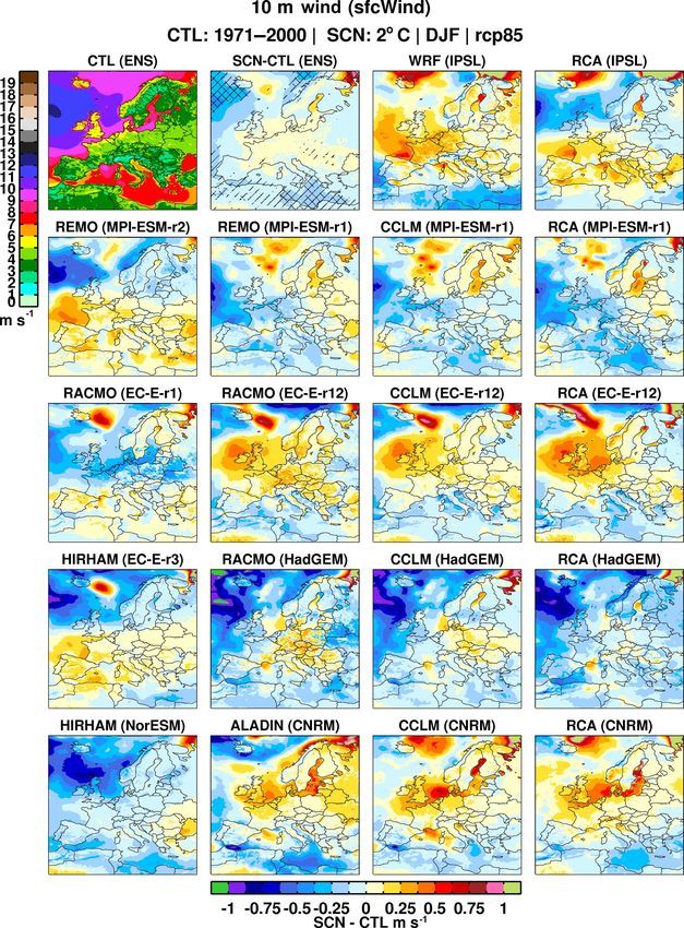
460                   E. Kjellström et al.: European climate change at global mean temperature increases of 1.5 and 2 ◦ C

1   Introduction                                                   project (Jacob et al., 2014). Previous works have shown that
                                                                   the high-resolution 12.5 km simulations add value compared
                                                                   to the 50 km simulations, in particular in terms of represent-
A main aim of the Paris agreement within the UNFCCC                ing extremes like heavy-precipitation events (e.g. Kotlarski
(United Nations Framework Convention on Climate Change)            et al., 2014; Prein et al., 2016). Other studies describing eval-
is to keep the increase in the global average temperature well     uation of different important near-surface variables in the
below 2 ◦ C above pre-industrial levels and to pursue efforts to   EURO-CORDEX RCMs in the recent past climate include
limit the temperature increase to 1.5 ◦ C above pre-industrial     those of Smiatek et al. (2016), Knist et al. (2016) and Frei
levels (UNFCCC, 2015). While the agreement comes into              et al. (2018).
power in 2020 we observe ongoing global warming with the              The relatively large ensemble of EURO-CORDEX high-
most recent years continuing the long-term warming trend of        resolution RCM climate change scenarios constitutes a valu-
the last decades (WMO, 2017). Regional and local impacts of        able data set for impact studies. Some of these simulations
global warming are already seen and there is a strong concern      and from the earlier ENSEMBLES project have been used
that these impacts will become worse with stronger future          for considerations of climate change at different warming
climate change (IPCC, 2014). However, exactly how strong           levels (e.g. Vautard et al., 2014; Maule et al., 2017) and in im-
these impacts will be at different warming levels is uncertain     pact studies (e.g. Alfieri et al., 2015; Donnelly et al., 2017).
as information about the climate change signal on a regional       However, previous studies have either been based on ear-
level is scarce. Despite some efforts that have been made to       lier RCM ensembles or only on smaller subsets of the full
look at possible climate change at 1.5 or 2 ◦ C of global warm-    EURO-CORDEX set of RCM simulations. In this study we
ing and to compare differences at these global warming levels      therefore focus on how the European climate may change
(e.g. Vautard et al., 2014; Fischer and Knutti, 2015; Schleuss-    at the 1.5 or 2 ◦ C of global warming levels in the larger
ner et al., 2016; King and Karoly, 2017), detailed information     set of EURO-CORDEX simulations at 12.5 km grid spacing.
about regional climate change is largely missing for scenar-       Specifically, we address at which of the two warming levels
ios reflecting 1.5 ◦ C of global warming (e.g. Mitchell et al.,    we can detect significant climate change compared to a refer-
2016).                                                             ence period in the end of the 20th century and to what extent
   Much of the available information about future regional         changes at the two warming levels differ, which is impor-
climate change comes from global climate models (GCMs).            tant for mitigation considerations. We also show how differ-
The most comprehensive set of GCM data is that of the              ent sources of uncertainty influence the climate change signal
CMIP5 (fifth phase of the Coupled Model Intercomparison            and discuss how the EURO-CORDEX simulations relate to
Project; e.g. Taylor et al., 2012) consisting of more than         the larger CMIP5 GCM ensemble.
30 GCMs. An advantage with GCMs is that they can pro-
vide regional information for all areas in the world. A lim-
                                                                   2     Methods and material
itation, however, is the fact that they are commonly oper-
ated at relatively coarse horizontal resolution (most often at
                                                                   2.1    Climate model simulations
100–200 km grid spacing). This implies that land–sea con-
trasts and land surface properties including mountain height       We use RCM data from 18 EURO-CORDEX simulations for
are only described in a coarse way and that important phe-         the European area; see Table 1 and Fig. 1. Specifically, we
nomena like mid-latitude cyclones and mesoscale processes          analyse seasonal mean, 2 m temperature, precipitation, wind
are handled in a rudimentary way. Dynamical downscaling            speed and mean sea level pressure (MSLP) for all RCMs
with regional climate models (RCMs) is one way of provid-          with the exception of WRF, for which MSLP data are miss-
ing high-resolution climate information that better accounts       ing. All RCM simulations have been performed with forc-
for regional to local scales and thereby adds value compared       ing following RCP8.5 (Representative Concentration Path-
to the GCM (e.g. Rummukainen, 2010; Sørland et al., 2018).         way; see Moss et al., 2010). The chosen simulations allow
For Europe, relatively large data sets of RCM scenarios have       us to address the impact of different driving GCMs on the
previously been put forward within the context of Euro-            resulting climate change signal. In addition, the impact of
pean research projects including PRUDENCE (Christensen             the choice of different RCMs can be investigated for both
et al., 2007; Déqué et al., 2007) and ENSEMBLES (van der           the three-member RCM ensembles downscaling MPI-ESM-
Linden and Mitchell, 2009; Déqué et al., 2012; Kjellström          LR-r1, EC-Earth-r12, HadGEM2-ES, and CNRM-CM5 and
et al., 2013). In recent years RCMs have been operated in          for the two-member ensemble downscaling IPSL-CM5A-
the framework of CORDEX (Coordinated Regional Climate              MR. Furthermore, as three members of EC-EARTH and two
Downscaling Experiment; e.g. Jones et al., 2011; Gutowski          members of MPI-ESM-LR are included, the role of inter-
et al., 2016). For Europe in particular, this means that an un-    nal natural variability can also be addressed. The simulations
precedented data set of RCM scenarios at 50 and 12.5 km            have been chosen based on the availability of data at the Earth
horizontal resolution is available from the EURO-CORDEX            System Grid Federation (ESGF) facility.

Earth Syst. Dynam., 9, 459–478, 2018                                                   www.earth-syst-dynam.net/9/459/2018/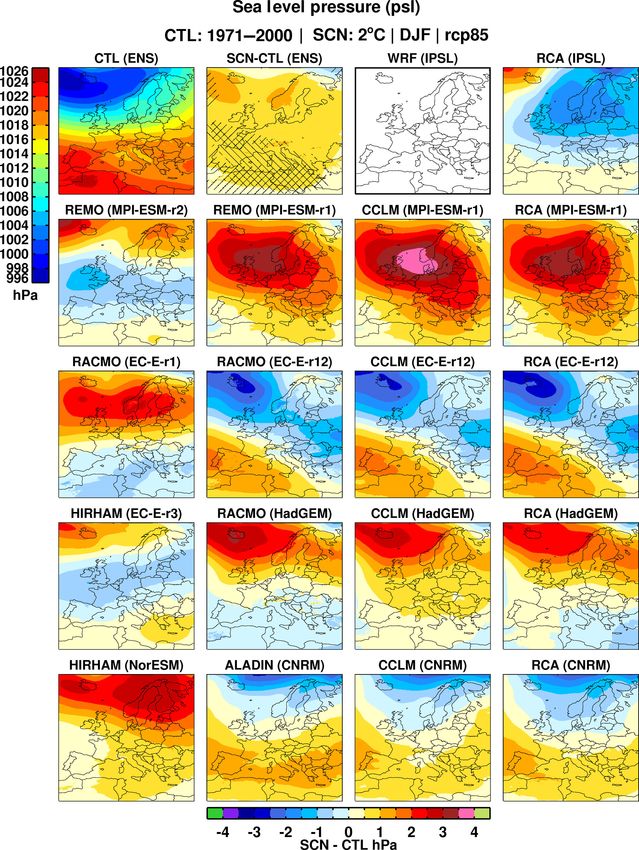
E. Kjellström et al.: European climate change at global mean temperature increases of 1.5 and 2 ◦ C                                461

Table 1. Regional climate model simulations assessed in this report. GCMs are listed in more detail in Table 2.

                   No.    Institute         RCM               GCM                 RCM reference
                   1      SMHI              RCA4              EC-EARTH-r12        Kjellström et al. (2016)
                   2                                          HadGEM2-ES
                   3                                          MPI-ESM-LR-r1
                   4                                          CNRM-CM5
                   5                                          IPSL-CM5A-MR
                   6      BTU Cottbus       CCLM4-8-17        EC-EARTH_r12        Keuler et al. (2016)
                   7                                          CNRM-CM5
                   8                                          MPI-ESM-LR-r1
                   9      ETH               CCLM4-8-17        HadGEM2-ES          Keuler et al. (2016)
                   10     HZG-GERICS        REMO2009          MPI-ESM-LR-r1       Jacob et al. (2012)
                   11                                         MPI-ESM-LR-r2
                   12     KNMI              RACMO2.2          EC-EARTH-r1         van Meijgaard et al. (2012)
                   13                                         EC-EARTH-r12
                   14                                         HadGEM2-ES
                   15     DMI               HIRHAM5           EC-EARTH-r3         Christensen et al. (1998)
                   16                                         NORESM1-M
                   17     CNRM              ALADIN53          CNRM-CM5            Colin et al. (2010); Bador et al. (2017)
                   18     IPSL              WRF3.3.1          IPSL-CM5A-MR        Skamarock et al. (2008)

                                                                           RCM results are set in a larger context by comparing to
                                                                        31 simulations from the CMIP5 multi-model GCM ensemble
                                                                        (Table 2). In addition to the nine GCM simulations listed in
                                                                        Table 1, the first ensemble members of the other 22 CMIP5
                                                                        GCMs are also assessed for seasonal mean changes in pre-
                                                                        cipitation and temperature. In this way we can investigate
                                                                        how the smaller subset of GCMs that provides input for the
                                                                        RCMs replicates the larger CMIP5 GCM ensemble. We can
                                                                        also look at if, and to what extent, the RCMs modify the
                                                                        climate change signal compared to that in the underlying
                                                                        GCMs. Comparisons are performed for a number of regions
                                                                        in Europe previously used in a large number of studies (e.g.
                                                                        Rockel and Woth, 2007; Christensen et al., 2010; Kjellström
                                                                        et al., 2013; Keuler et al., 2016), see Fig. 1.

                                                                        2.2   Calculation of warming levels
                                                                        We investigate periods for which the global mean near-
                                                                        surface temperature is 1.5 or 2.0 ◦ C above pre-industrial con-
                                                                        ditions (hereafter referred to as SWL1.5 and SWL2, where
                                                                        SWL stands for specific warming level). As the temperature
                                                                        in true pre-industrial, i.e. pre-1750, conditions are not known
                                                                        (see Hawkins et al., 2017; Schurer et al., 2017), we use the
                                                                        simulated climate from the GCMs for 1861–1890 as a proxy.
Figure 1. Map showing the eight subdomains (BI – the British            For each GCM we then identify the first period when the 30-
Isles; IP – the Iberian Peninsula; FR – France; ME – mid-Europe;
                                                                        year running mean global temperature reaches 1.5 or 2.0 ◦ C
SC – Scandinavia; MD – the Mediterranean region; AL – the Alps;
                                                                        above that of the pre-industrial period. These 30-year time
EA – eastern Europe) and the larger European domain for which
average climate change signals have been calculated. The colours        slices (see Table 2) are used for the analyses in the study (see
represent the altitude of the surface in the RCA4 model at the 0.11◦    for details Nikulin et al., 2018). For comparing future climate
EURO-CORDEX grid.                                                       change we then use the period 1971–2000 as our reference in
                                                                        the RCM simulations. This choice is made as (i) the starting
                                                                        point (1971) is the first possible as not all RCMs have data
                                                                        for earlier years and (ii) the end point (2000) is before the

www.earth-syst-dynam.net/9/459/2018/                                                           Earth Syst. Dynam., 9, 459–478, 2018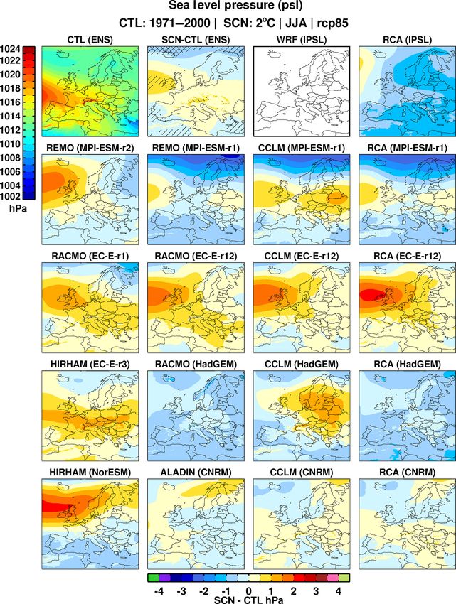
462                    E. Kjellström et al.: European climate change at global mean temperature increases of 1.5 and 2 ◦ C

Table 2. CMIP5 GCMs assessed here. Columns SWL1.5 and SWL2 show the central year in a 30-year period when GCMs reach the 1.5 and
2 ◦ C of warming levels (i.e. 2030 represents 2016–2045) under RCP8.5. GCMs are listed in order of when they reach SWL2. Only ensemble
member r1 has been used unless otherwise noted in brackets after the GCM name. GCMs in italics have been downscaled by RCMs (see
Table 1). For more information see Taylor et al. (2012) and https://pcmdi.llnl.gov/mips/cmip5/ (last access: 27 April 2018).

  No.    Institute                                                                      GCM name                SWL 1.5     SWL2
  1      Beijing Normal University                                                      BNU-ESM                 2009        2023
  2      Canadian Centre for Climate Modelling and Analysis                             CanESM2                 2013        2026
  3      Institut Pierre-Simon Laplace                                                  IPSL-CM5A-LR            2011        2027
  4      Atmosphere and Ocean Research Institute (The University of Tokyo)              MIROC-ESM               2020        2030
  5      National Institute for Environmental Studies, and Japan Agency for Marine-     MIROC-ESM-CHEM          2018        2030
         Earth Science and Technology
  6      National Center for Atmospheric Research                                       CCSM4                   2013        2030
  7      Institut Pierre-Simon Laplace                                                  IPSL-CM5A-MR            2016        2030
  8      Max Planck Institute for Meteorology                                           MPI-ESM-LR (r2)         2016        2032
  9      NASA/GISS (Goddard Institute for Space Studies)                                GISS-E2-H-CC            2017        2035
  10     EC-EARTH consortium                                                            EC-EARTH (r1)           2017        2035
  11     Geophysical Fluid Dynamics Laboratory                                          GFDL-CM3                2023        2035
  12     Max Planck Institute for Meteorology                                           MPI-ESM-LR (r2)         2018        2035
  13     EC-EARTH consortium                                                            EC-EARTH (r12)          2019        2035
  14     NASA/GISS (Goddard Institute for Space Studies)                                GISS-E2-H               2020        2036
  15     EC-EARTH consortium                                                            EC-EARTH (r3)           2020        2037
  16     Institut Pierre-Simon Laplace                                                  IPSL-CM5B-LR            2022        2037
  17     Met Office Hadley Centre                                                       HadGEM2-ES              2024        2037
  18     Max Planck Institute for Meteorology                                           MPI-ESM-MR              2020        2038
  19     Met Office Hadley Centre                                                       HadGEM2-CC              2029        2041
  20     The First Institute of Oceanography, SOA                                       FIO-ESM                 2027        2042
  21     Centre National de Recherches Météorologiques/Centre Européen de               CNRM-CM5                2029        2043
         Recherche et Formation Avancée en Calcul Scientifique
  22     Commonwealth Scientific and Industrial Research Organization/Queensland        CSIRO-Mk3-6-0           2032        2044
         Climate Change Centre of Excellence
  23     Met Office Hadley Centre                                                       HadGEM2-AO              2034        2046
  24     Norwegian Climate Centre                                                       NorESM1-ME              2032        2046
  25     NASA/GISS (Goddard Institute for Space Studies)                                GISS-E2-R-CC            2031        2048
  26     Norwegian Climate Centre                                                       NorESM1-M               2033        2048
  27     Atmosphere and Ocean Research Institute (The University of Tokyo), National    MIROC5                  2033        2048
         Institute for Environmental Studies, and Japan Agency for Marine-Earth Sci-
         ence and Technology
  28     NOAA Geophysical Fluid Dynamics Laboratory                                     GFDL-ESM2M              2034        2051
  29     Meteorological Research Institute                                              MRI-CGCM3               2040        2052
  30     Geophysical Fluid Dynamics Laboratory                                          GFDL-ESM2G              2037        2054
  31     Russian Academy of Sciences, Institute of Numerical Mathematics                inmcm4                  2043        2058

first year in any of the 30-year SWL1.5 time periods down-           2.3   Estimation of consistency and robustness of the
scaled here (the IPSL model, number 7 in Table 2). From ob-                simulated climate change signal
servations we note that the global warming between 1861–
1890 (pre-industrial) and 1971–2000 (reference) is 0.41 ◦ C
                                                                     We calculate differences among 30-year periods as described
according to HadCRUT4 (Morice et al., 2012), implying that
                                                                     above and we let the mean over the ensemble members rep-
future temperature changes above 1.1 and 1.6 ◦ C represent
                                                                     resent the climate change signal for the different variables
a regional warming exceeding the global average for the two
                                                                     investigated. Further, we consider the climate change signal
warming levels.
                                                                     to be consistent if at least 80 % of the simulations (14 out of
                                                                     the 18) agree on the sign of climate change. In areas where
                                                                     the climate change signal is found to be consistent we term
                                                                     the change robust if the signal-to-noise ratio is equal to 1 or
                                                                     larger. Here, the signal-to-noise ratio is defined as the ratio
                                                                     between the mean ensemble change divided by 1 SD calcu-

Earth Syst. Dynam., 9, 459–478, 2018                                                      www.earth-syst-dynam.net/9/459/2018/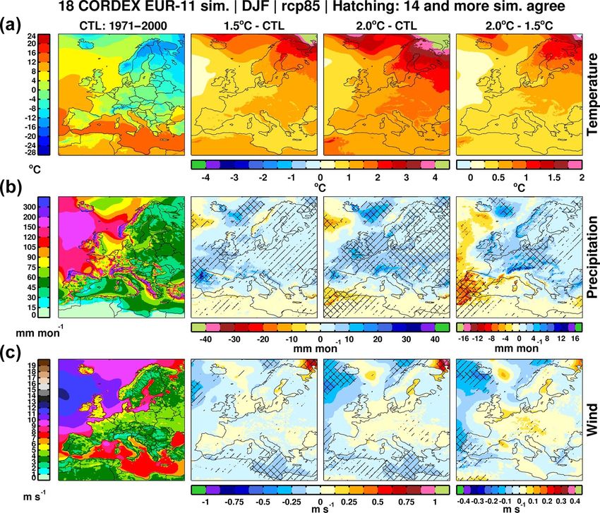
E. Kjellström et al.: European climate change at global mean temperature increases of 1.5 and 2 ◦ C                        463

lated over the changes in the individual ensemble members.       Also, CNRM-CM5 indicates a strengthening of the gradient
These characteristics are calculated for both the RCMs and       although not as strong. The MPI-ESM-LR-r2-driven simula-
the underlying GCMs.                                             tion and the EC-EARTH-r3-driven run both show decreasing
                                                                 MSLP over the British Isles and in a band over the European
3     Results                                                    continent, indicating a southward shift of the storm track. Fi-
                                                                 nally, IPSL-CM5A-MR shows a very different pattern with
Here we compare simulated changes at SWL1.5 and SWL2             lower pressure in general over large parts of northern Europe,
for seasonal mean near-surface temperatures and precipita-       indicating a stronger low-pressure activity in this area.
tion and wind speed over Europe for winter (December–               Also, for summer the change patterns differ. Several sim-
February, DJF) and summer (June–August, JJA). We focus           ulations indicate a strengthening and/or northward displace-
on RCM results in the main text; comparable results from         ment of the subtropical high (the two MPI-ESM-LR mem-
the underlying GCMs are given as the Supplement. First,          bers, all EC-EARTH members and NorESM1-M). In MPI-
however, we show how changes in MSLP differ among the            ESM-LR-r1 the strengthened subtropical high is also associ-
individual ensemble members as these changes are known           ated with a decrease in pressure in the northernmost part of
to have strong impacts on changes in the other variables         the Atlantic and over Scandinavia. This pattern is indicative
(e.g. Van Ulden and van Oldenborgh, 2006; Kjellström et al.,     of a northward shift of the storm track in summer. Five out of
2011; Aalbers et al., 2017).                                     the six GCM simulations with a strengthening of the subtrop-
                                                                 ical high show a reinforcement of this signal with warming
                                                                 as the MSLP anomalies are larger at SWL2 than at SWL1.5
3.1    Simulated changes in MSLP
                                                                 (not shown). A similar pattern with reinforcements in MSLP
Figures 2 and 3 show the changes in MSLP in each ensem-          changes when looking at SWL2 compared to SWL1.5 is not
ble member at SWL2 for winter and summer respectively            generally seen in winter. This contrast between the two sea-
(apart from WRF for which MSLP data are missing. We              sons indicates that changes in winter are more associated
have, however, included a blank panel for WRF for consis-        with internal variability while summertime changes are to
tency with later figures). It is clear that there are consid-    a larger degree associated with long-term global warming.
erable differences among the different simulations and that
these differences are closely connected to both the choice       3.2   Simulated changes in near-surface temperature
of GCMs (e.g. comparing CNRM-CM5-driven simulations
with those driven by HadGEM2-ES) but also to the choice          Warming is manifested in all seasons as exemplified for win-
of ensemble member (as illustrated by the two realizations       ter and summer in Figs. 4 and 5 (and correspondingly for the
of MPI-ESM-LR or the three EC-EARTH members). Fur-               underlying GCM ensemble in Figs. S1 and S2). The large-
ther, we note that there are some but weaker differences also    scale features are to a strong degree very similar among the
due to the RCM. The latter can be seen from the six pan-         RCMs and the underlying GCMs. A number of regional fea-
els showing the RACMO, CCLM and RCA4 simulations                 tures stand out from the figures, including a stronger warm-
downscaling EC-EARTH-r12 and HadGEM2-ES. The most                ing in winter than in summer in large parts of northeastern
pronounced difference in winter is the stronger increase in      Europe, while the strongest warming in summer is found in
MSLP in southern and central Europe in the HadGEM2-ES-           the south and southwest but also in parts of Scandinavia. This
driven CCLM simulation compared to the two others (Fig. 2).      is consistent with the findings of Vautard et al. (2014), who
Also, for summer this CCLM simulation differs compared to        analysed a different set of simulations and scenarios for the
the two other RCMs in showing an increase in MSLP in large       time when global mean temperatures have increased by 2 ◦ C
parts of eastern Europe and the Baltic Sea region (Fig. 3).      compared to pre-industrial conditions. Changes are generally
   In winter we note that the strong north–south pressure        smaller over the oceans than over land areas, with the excep-
gradient over the North Atlantic is changed differently in       tion of some parts of the northern seas that show very strong
the different simulations (Fig. 2). In the southern half of      warming mainly in winter but also to some extent in summer.
the domain in the MPI-ESM-LR-r1-driven simulations there         This strong warming over the northern seas can to a large de-
is a weakening in this pressure gradient, while it is inten-     gree be attributed to reduction in sea ice in the warmer cli-
sified in the north. This indicates a northward shift in the     mate. The stronger warming in summer over the Baltic Sea
storm track with less (more) mild air being advected in over     than over its surroundings, however, cannot be directly re-
central and southern Europe (northern Scandinavia) from          lated to changes in sea ice as there is none in the Baltic Sea
the Atlantic. Similar patterns are seen in the simulations       in summer. We have not investigated the reason for the Baltic
driven by HadGEM2-ES, NorESM1-M and in EC-EARTH-                 Sea warming in detail here but we note that it is larger in
r1. Contrastingly, EC-EARTH-r12 shows a completely dif-          some GCM-driven experiments than others (not shown) so
ferent pattern with a strengthening of the north–south pres-     it is likely that the boundary forcing from the GCMs is the
sure gradient, albeit with no major relocation of it, indicat-   cause. A comparison of the climate change signal at the two
ing a strengthening of the westerlies over the North Atlantic.   warming levels shows considerably larger changes at SWL2

www.earth-syst-dynam.net/9/459/2018/                                                 Earth Syst. Dynam., 9, 459–478, 2018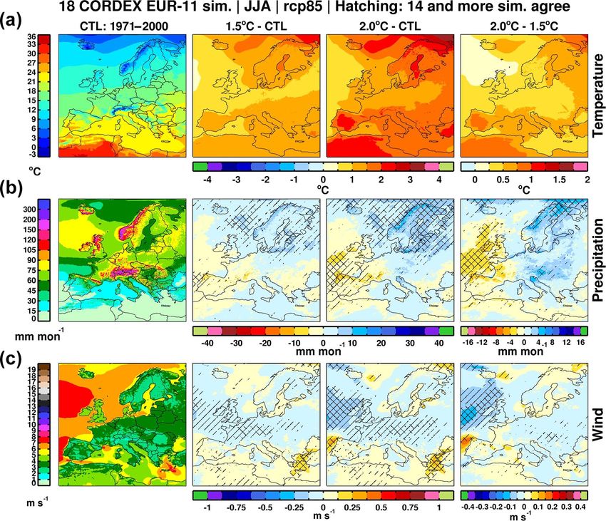
464                    E. Kjellström et al.: European climate change at global mean temperature increases of 1.5 and 2 ◦ C

Figure 2. Winter (DJF) mean sea level pressure in the reference period (ensemble mean in the uppermost left panel) and its change in 17
RCM simulations in Table 1 (individual runs in upper right panel and all other rows) for the +2 ◦ C of warming level (SWL2). As MSLP
data for the WRF simulation are missing, that panel is left blank. Hatching in the ensemble mean signal (second upper panel from the left)
represents areas where at least 14 of the 18 ensemble members agree on the sign of change. Cross-hatching indicates that there is agreement
on the sign of change and that the signal-to-noise ratio is larger than 1.

than at SWL1.5. The regional patterns of the differences be-            peratures in both seasons already at SWL1.5. It is only in
tween the two warming levels closely follow the regional pat-           winter that a few (one to three) ensemble members display
terns of change outlined above. The results show large areas            a weak decrease at SWL1.5 over parts of eastern Europe
seeing more than 0.5 ◦ C of additional warming at SWL2. In              and Scandinavia while almost all individual simulations also
winter, over northern Scandinavia, additional warming ex-               show warming in all these areas at SWL2 (not shown). Apart
ceeding 1 ◦ C is noted compared to that at SWL1.5 (Fig. 4).             from these exceptions over the continent, a few simulations
   Figures 4 and 5 reveal that temperature increase is a highly         also show the absence of warming over parts of the Atlantic
consistent feature of the RCM–GCM combinations assessed                 west of the British Isles as a result of a weaker warming in
here as basically all 18 simulations indicate increasing tem-           the underlying GCMs in this area. Despite the agreement on

Earth Syst. Dynam., 9, 459–478, 2018                                                         www.earth-syst-dynam.net/9/459/2018/
E. Kjellström et al.: European climate change at global mean temperature increases of 1.5 and 2 ◦ C                                   465

Figure 3. Summer (JJA) mean sea level pressure in the reference period (ensemble mean in the uppermost left panel) and its change in 17
RCM simulations in Table 1 (individual runs in the upper right panel and all other rows) for the +2 ◦ C of warming level (SWL2). Hatching
in the ensemble mean signal (second upper panel from the left) represents areas where at least 14 of the 18 ensemble members agree on the
sign of change. Cross-hatching indicates that there is agreement on the sign of change and that the signal-to-noise ratio is larger than 1.

sign there are still large differences among individual sim-            weaker southwesterlies over large parts of the North At-
ulations in some areas (not shown). This is most notable in             lantic, we interpret this relatively modest warming as a con-
the far north over ocean areas in winter which is the area              sequence of the changing large-scale circulation bringing
in Europe warming the most (see Fig. 4). Apart from the                 less mild Atlantic air in over Europe. Similarly, we can in-
far north we also note relatively large spread in southeast-            terpret the larger temperature increase in the EC-EARTH-
ern Europe in winter at both warming levels. A closer look at           r12-driven RACMO simulation over large parts of Europe
the individual simulations reveals that the three MPI-ESM-              compared to the corresponding EC-EARTH-r1-driven one
LR-r1-driven simulations all give very modest warming, or               with the changes in MSLP discussed above. Apart from
even local cooling, for both SWL1.5 and SWL2 (not shown).               these GCM-driven differences we also note differences aris-
Recalling the changes in MSLP (Fig. 2) with, on average,                ing from choice of RCMs. For instance we note that RCA4

www.earth-syst-dynam.net/9/459/2018/                                                          Earth Syst. Dynam., 9, 459–478, 2018
466 E. Kjellström et al.: European climate change at global mean temperature increases of 1.5 and 2 ◦ C
Figure 4. Ensemble mean winter (DJF) 2 m temperature (a), precipitation (b) and 10 m wind speed (c) in the control period (left), its change
at SWL1.5 (second column) and SWL2 (third column), and the difference between the change at SWL2 and SWL1.5 (rightmost column).
Hatching in the climate change signal for precipitation and wind speed represents areas where at least 14 of the 18 ensemble members agree
on the sign of change (for temperature this is always the case). Cross-hatching indicates that there is agreement on the sign of change and
that the signal-to-noise ratio is larger than 1. Hatching in the rightmost plots indicates that changes at SWL2 are larger than those at SWL1.5
in at least 14 of the models.
shows stronger warming than CCLM in eastern Europe in resolution in the RCMs gives rise to more pronounced dif-
winter when forced by EC-EARTH-r12 as does RACMO in ferences in coastal and mountainous areas than in the GCMs
the HadGEM2-ESM-driven one (not shown). Similarly, AL- as the stronger orographic contrasts can amplify the changes.
ADIN shows stronger warming in summer in southeastern Apart from this, the large-scale features are generally similar
Europe than both CCLM and RCA4 when forced by CNRM- in the GCMs and in the RCMs. Changes generally increase
CM5. These differences among the RCMs indicate some over time and the extent of areas showing consistent and ro-
systematic difference among them and how they respond to bust changes increases from SWL1.5 and SWL2. However,
changes in the large-scale forcing. in some areas changes at SWL2 are smaller than those at
SWL1.5. As an example the Iberian Peninsula and the adja-
cent North Atlantic show strong increases in wintertime pre-
3.3 Simulated changes in precipitation cipitation already at SWL1.5 while there is no additional in-
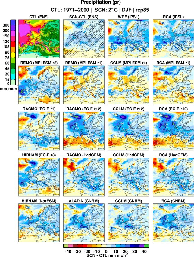
Precipitation changes in the analysed simulations follow the crease (or even a weaker signal indicating decrease between
well-known pattern for Europe, with tendencies for increas- the two periods) at SWL2. Compared to the findings for tem-
ing precipitation in the north and decreases in the south perature, precipitation changes are less robust. Notably, there
on an annual mean basis (not shown). The borderline be- are relatively large areas without hatching on the maps where
tween increasing and decreasing precipitation migrates from different RCM simulations show either an increase or a de-
a southerly position in winter (Figs. 4 and S1) to a northerly crease in precipitation. We also note that in areas where there
position in summer (Figs. 5 and S2). As expected, the higher is partial consensus of 14–15 models or more on the sign of
Earth Syst. Dynam., 9, 459–478, 2018 www.earth-syst-dynam.net/9/459/2018/E. Kjellström et al.: European climate change at global mean temperature increases of 1.5 and 2 ◦ C 467
Figure 5. Ensemble mean summer (JJA) 2 m temperature (a), precipitation (b) and 10 m wind speed (c) in the control period (left), its change
at SWL1.5 (second column) and SWL2 (third column), and the difference between the change at SWL2 and SWL1.5 (rightmost column).
Hatching in the climate change signal for precipitation and wind speed represents areas where at least 14 of the 18 ensemble members agree
on the sign of change (for temperature this is always the case). Cross-hatching indicates that there is agreement on the sign of change and
that the signal-to-noise ratio is larger than 1. Hatching in the rightmost plots indicates that changes at SWL2 are larger than those at SWL1.5
in at least 14 of the models.
the change there can still be large uncertainties related to the tion changes. The northward shift in the storm track in sum-
amplitude of the change (Fig. 6). mer (see Fig. 3) is reflected by strong increases in precipi-
In some more detail it is clear that some of the differences tation in parts of Scandinavia (Fig. 5). In southern and cen-
in precipitation response are strongly related to changes in tral Europe, however, there is a reduction in precipitation in
the large-scale circulation. As an example, a comparison connection with the northward displacement of the subtrop-
of Figs. 6 and 2 reveals that decreasing precipitation over ical high and increasing MSLP over Europe. Again, there
the North Atlantic south of Iceland in the HadGEM2-ES- are also large differences among individual RCMs when
and MPI-ESM-r1-driven simulations is connected to higher forced by the same driving GCM simulation. Examples in-
MSLP and weaker north–south pressure gradients, a pattern clude stronger increases in precipitation in RCA4 compared
that is indicative of weaker westerly winds and less cyclone to CCLM and RACMO in northern Scandinavia (not shown).
activity in this area. Contrastingly, the stronger N–S pres-
sure gradient over the Atlantic in the EC-EARTH-r12-driven
3.4 Simulated changes in near-surface wind speed
simulations, and to a lesser extent in the CNRM-CM5-driven
simulations, leads to stronger westerlies and substantial in- The simulated climate change signal in mean near-surface
creases in precipitation over this region. These regional-scale wind speed is generally not consistent over Europe. De-
positive and negative changes in precipitation are more pro- creases are seen over parts of the North Atlantic and the
nounced over parts of the British Isles and southern Norway, Mediterranean in winter (Figs. 4 and S1) and over parts of
which is indicative of orographic amplification of precipita- the North Atlantic and western Europe in summer (Figs. 5
www.earth-syst-dynam.net/9/459/2018/ Earth Syst. Dynam., 9, 459–478, 2018468 E. Kjellström et al.: European climate change at global mean temperature increases of 1.5 and 2 ◦ C Figure 6. Winter (DJF) precipitation in the reference period (ensemble mean in the uppermost left panel) and its change in 18 RCM simulations in Table 1 (two uppermost right panels and all other rows) for the +2 ◦ C of warming level (SWL2). Hatching in the ensemble mean signal (second upper panel from the left) represents areas where at least 14 of the 18 ensemble members agree on the sign of change. Cross-hatching indicates that there is agreement on the sign of change and that the signal-to-noise ratio is larger than 1. and S2), confirming the results of Tobin et al. (2016). In- in large parts of the area, while the sharpening of the gradi- creases are seen over some northern ocean areas, most no- ent in the EC-EARTH-r12-driven simulations leads to strong tably in the RCMs but to some extent also in the GCMs. increases in wind speed in the area of the British Isles (com- These are strongest in winter but can to some extent be seen pare Figs. 2 and 7). Apart from these changes that are related in all seasons. A closer look at the individual simulations re- to changes in the large-scale circulation, there are also other veals that there are strong connections to the variability in the wind speed changes. Figure 7 reveals that the local increases large-scale circulation as indicated by changes in the MSLP over parts of the northern oceans are seen in most simulations pattern. Notably, the weakening and northward shift in the although at slightly different locations. There are no com- N–S pressure gradient in the HadGEM2-ES-driven simula- mon changes in MSLP that can explain this pattern. How- tions is reflected in a considerable decrease in wind speed ever, we note strong increases in near-surface temperature in Earth Syst. Dynam., 9, 459–478, 2018 www.earth-syst-dynam.net/9/459/2018/
E. Kjellström et al.: European climate change at global mean temperature increases of 1.5 and 2 ◦ C                                 469

Figure 7. Winter (DJF) 10 m wind speed in the reference period (ensemble mean in the uppermost left panel) and its change in 18 RCM
simulations in Table 1 (two uppermost right panels and all other rows) for the +2 ◦ C of warming level (SWL2). Hatching in the ensemble
mean signal (second upper panel from the left) represents areas where at least 14 of the 18 ensemble members agree on the sign of change.
Cross-hatching indicates that there is agreement on the sign of change and that the signal-to-noise ratio is larger than 1.

these areas in the models (not shown). This strong relation            wind speed over the Arctic Ocean areas in some simulations
between near-surface temperature and winds indicates that              (not shown). However, we also note similar differences in
changing surface conditions are important here. The reduc-             some simulations over the Baltic Sea where sea ice cannot
tion of sea ice and the associated higher temperatures likely          be the reason for summertime differences. Changes in wind
lead to a less stably stratified planetary boundary layer that         speed are more pronounced in some areas at SWL2 than at
thereby becomes more favourable for downward mixing of                 SWL1.5, indicating that we are looking at a manifestation of
momentum leading to higher wind speed close to the surface.            long-term climate change. However, we note that the areas
Also in summer, changes in sea ice and associated changes in           where models agree upon sign of change in wind speed do
sea surface temperatures (SSTs) may contribute to increasing           not become considerably larger at SWL2 and that large areas

www.earth-syst-dynam.net/9/459/2018/                                                         Earth Syst. Dynam., 9, 459–478, 2018
470                    E. Kjellström et al.: European climate change at global mean temperature increases of 1.5 and 2 ◦ C

do not show any systematic changes in wind speed reflecting         for these variables, but there are still large areas where such
the importance of internal variability. In summary, the results     changes are not evident.
indicate that it is highly uncertain what may happen to wind           The results indicate that the large-scale circulation has an
speed in this region when global warming continues.                 important role in determining the actual climate change sig-
                                                                    nal in any individual simulation. For instance, it is clear that
                                                                    stronger westerlies in some simulations are associated with
4     Discussion
                                                                    milder and wetter conditions over parts of the continent while
4.1    Is there a detectable climate change signal in the
                                                                    weaker westerlies are associated with less precipitation along
       EURO-CORDEX ensemble at 1.5 and 2 ◦ C of global
                                                                    the western coastlines. This is in concert with previous stud-
       warming?
                                                                    ies showing a similar dependence (e.g. Van Ulden and van
                                                                    Oldenborgh, 2006; Kjellström et al., 2011; Kjellström et al.,
The results of the 18 RCM simulations analysed here show            2013). Differences in the large-scale circulation over decade-
increasing temperatures, changing precipitation patterns and        long climate simulations are not necessarily a sign of climate
also some changes in seasonal mean wind speed (Figs. 4 and          change but rather a manifestation of the large internal vari-
5). These changes are more or less consistent and robust for        ability in the climate system that can be pronounced on a re-
the different variables. The ensemble mean shows consistent         gional scale (e.g. Hawkins and Sutton, 2009). As our results
and robust changes in all land areas already at SWL1.5 for          are based on a relatively small number of GCM simulations
both seasons (Table 3), and temperature increases are sim-          we are limited in the degree to which the ensemble captures
ulated in all parts of Europe for all seasons by all individ-       the full uncertainty. Larger ensembles consisting of multi-
ual models (not shown). Differences between SWL1.5 and              ple simulations with one, or preferably many models, would
SWL2 amount to somewhere between 0.3 and 0.8 ◦ C for                provide a better opportunity to sample this uncertainty (e.g.
summer and winter seasonal mean conditions averaged over            Deser et al., 2012; Aalbers et al., 2017). It is clear that the nat-
the different regions in Fig. 1 (compare Table 4 and S1). Pre-      ural variability with its impacts on the large-scale circulation
cipitation changes show larger model spread, and ensemble           is a major cause of uncertainty. This is highly pronounced
mean changes at SWL1.5 are consistent and robust in only            when it comes to assessing climate change signals at any of
less than 10 % of the European land areas (Table 3). Despite        the two warming levels discussed here as changes still do
generally larger changes, this fraction is also relatively small    not, even if robust and seen in most simulations, necessarily
at SWL2 and it is not until higher warming levels (2.5 and          exceed the natural variability.
3 ◦ C above pre-industrial conditions) that the ensemble mean
signal is consistent and robust in more than half of Europe for     4.2   Timing for reaching 1.5 and 2 ◦ C above
winter. For summer this still only applies for less than 25 %             pre-industrial conditions
of the European land areas even at 3 ◦ C of warming. This
low degree of consistency and robustness reflects the uncer-        An alternative approach to the one used here for investigat-
tainties even in sign of change in the seasonally migrating         ing climate change at the time of 1.5 and 2 ◦ C of warm-
area between increasing precipitation in the north and de-          ing would be to use scenarios in which the climate system
creasing precipitation in the south. For wind speed there are       reaches a new equilibrium at the requested warming levels.
also large uncertainties with different models showing very         This could for instance be closer to the end of the century in
different response patterns, and the fraction of Europe for         scenarios with rapidly decreasing forcing and eventual stabi-
which there is a consistent and robust change is as low as          lization of the climate. A difficulty with that approach is that
that for precipitation in summer, while in winter it is even less   different GCMs with different climate sensitivities may ei-
(Table 3). We note that for the studied variables the ensem-        ther not reach the warming levels or exceed them. The defini-
ble mean changes at SWL2 are generally larger than those            tion of warming levels used here assures that the global mean
at SWL1.5. This is always the case for temperature, while           warming for the investigated periods is exactly 1.5 and 2 ◦ C
for precipitation and wind speed there are local exceptions         above pre-industrial conditions as simulated by the mod-
to this. Differences among individual ensemble members are          els. The choice of extracting this information from a tran-
often large, sometimes larger than the overall climate change       sient simulation implies that there will be trends in the time
signal at SWL1.5 and SWL2. It is evident that while a clear         slices that may influence the results (Bärring and Strandberg,
robust climate change signal is seen for temperature it has not     2018). For instance, interannual variability may be artificially
emerged in all other variables, seasons and regions studied         augmented in case of a long-term increasing (or decreasing)
here. This finding is in accordance with earlier studies that       trend. Such trends could be removed before investigating in-
have also shown different times of emergence of a regional          terannual variability or extreme conditions that may be sensi-
climate change signal (e.g. Giorgi and Bi, 2009; Hawkins and        tive to increased temporal variability. However, for this study
Sutton, 2012; Kjellström et al., 2013). Table 3 reveals that        we have chosen not to do this as we focus on long-term sea-
at even higher warming levels SWL2.5 and SWL3 the frac-             sonal averages. Another potential problem with the transient
tion of land with consistent and robust changes also increases      approach is when results are going to be used in impact stud-

Earth Syst. Dynam., 9, 459–478, 2018                                                     www.earth-syst-dynam.net/9/459/2018/
E. Kjellström et al.: European climate change at global mean temperature increases of 1.5 and 2 ◦ C 471
Table 3. Summary statistics showing the fraction of land in the larger European domain (see Fig. 1) where the ensemble members show
consistent changes (80 % agree on sign) and in addition show a robust change for four different warming levels between 1.5 and 3 ◦ C as
defined in Sect. 2.3. The numbers in parentheses represent the corresponding fraction from the underlying GCM ensemble.
1.5 ◦ C 2 ◦C 2.5 ◦ C 3 ◦C
Winter (DJF)
Temperature Consistent 100 (100) 100 (100) 100 (100) 100 (100)
Consistent and robust 100 (100) 100 (100) 100 (100) 100 (100)
Precipitation Consistent 47 (45) 67 (75) 75 (80) 79 (87)
Consistent and robust 9 (11) 40 (32) 64 (63) 67 (82)
Wind speed Consistent 7 (40) 10 (30) 14 (29) 13 (50)
Consistent and robust 0 (15) 1 (11) 3 (9) 3 (18)
Summer (JJA)
Temperature Consistent 100 (100) 100 (100) 100 (100) 100 (100)
Consistent and robust 100 (100) 100 (100) 100 (100) 100 (100)
Precipitation Consistent 24 (40) 37 (47) 44 (50) 53 (58)
Consistent and robust 4 (18) 15 (25) 18 (35) 25 (39)
Wind speed Consistent 32 (25) 45 (45) 51 (42) 52 (54)
Consistent and robust 7 (1) 14 (9) 25 (15) 27 (28)
ies for which there may be other important time constraints. Some GCMs have been run several times to sample the
A certain level of global climate change may have very dif- natural variability in the system and usually these ensemble
ferent regional signatures at different timings. For instance, members show slightly different results. The largest ensem-
Maule et al. (2017) shows that if the time it takes until a cer- ble of one GCM in the CMIP5 data set is the CSIRO model
tain warming level is reached is longer (as a result of weaker with 10 different members (member number 1 is shown in
forcing in RCP4.5), the regional climate change signal in Eu- Table 2). The central year for reaching the 1.5 ◦ C of warm-
rope is weaker than if the level is reached quickly (as result of ing level in that 10-member ensemble ranges between 2027
strong forcing in RCP8.5). Apart from such differences in re- and 2035. For the corresponding 2 ◦ C level it ranges be-
gional climate response, impacts will be different if changes tween 2041 and 2046. These relatively smaller intervals,
are quick or slow depending on the resilience of the consid- compared to those of the CMIP5 multi-model ensemble dis-
ered society or ecosystem. cussed above, indicate that the simulated natural variability
Here, we present information about when the two specific in the global mean temperature is a smaller source of un-
warming levels are reached given the data used in the study. certainty than that of the climate sensitivities as represented
A benefit of this transient, non-stabilized approach is that by the different GCMs. This does not, however, imply that
it represents conditions that may be more representative for natural variability on the regional scale is not important as
what happens if we do not meet the 2 ◦ C target (or 1.5 ◦ C for a source of uncertainty (as discussed in Sect. 4.1).
that matter). Even if global warming will be more than 2 ◦ C In addition to climate model sensitivity and natural vari-
it may be valuable to look at SWLs in an adaptation context, ability, different forcing also plays a role in when a certain
as a level of climate change that we will have to adapt to on warming level is reached. We note that the 30-year time slices
our way to the even warmer climate beyond 2 ◦ C. In that case used in the analysis here partly overlap between the two time
this approach is a way to shift the perspective from the rela- windows. For the RCP8.5 scenarios central years between
tively uncertain level of climate change at a specific point in the two periods differ by between 18 and 10 years in any of
time to a more certain level of climate change at an uncertain the GCM simulations, indicating that at least 12 years is com-
point in time. mon for the two time slices for any given simulation while for
Partly due to their different climate sensitivity the CMIP5 some model simulations a variation of even up to 20 years is
GCMs reach the different warming levels at different points the same. Clearly, the two samples are more similar com-
in time. For the 31 RCP8.5 runs in Table 1 the central years of pared to if they were taken as time slices more separated
the 30-year periods range between 2009 and 2043. The sub- from each other. This similarity has implications for how to
set of GCMs that has been downscaled in EURO-CORDEX assess differences between the periods in a statistically rigor-
and further assessed here shows central years ranging be- ous way as data in the two samples are not independent.
tween 2016 and 2029. Therefore, it is clear that the chosen All 31 GCMs in Table 2 have also been run for RCP4.5.
subset does not sample the full range of climate sensitivities For that scenario SWL1.5 is reached between 2008 and 2061
in the GCMs. in the different models (not shown). SWL2, however, is
www.earth-syst-dynam.net/9/459/2018/ Earth Syst. Dynam., 9, 459–478, 2018472 E. Kjellström et al.: European climate change at global mean temperature increases of 1.5 and 2 ◦ C
Table 4. Summary statistics showing temperature and precipitation changes at SWL1.5 for the eight regions in Fig. 1. For each region there
are three sets of data for each season and variable representing the full CMIP5 ensemble (top), the nine-member GCM ensemble downscaled
by the RCMs (middle) and the 18-member RCM ensemble (lower). The numbers represent the minimum (left), maximum (right) and mean
plus or minus 1 SD (middle) of the ensemble members’ individual area mean climate changes.
Near-surface temperature (◦ C) Precipitation (%)
DJF JJA DJF JJA
Area Min Mean ± SD Max Min Mean ± SD Max Min Mean ± SD Max Min Mean ± SD Max
IP 0.35 0.92 ± 0.35 1.67 0.58 1.42 ± 0.55 2.68 −17 −2.0 ± 8.9 19 −33 −7.8 ± 8.6 13
0.40 0.87 ± 0.40 1.67 0.74 1.16 ± 0.47 1.99 −3.6 5.6 ± 6.8 19 −21 −7.3 ± 8.6 9.4
0.35 0.79 ± 0.40 1.58 0.58 0.94 ± 0.32 1.59 −2.7 3.5 ± 5.3 19 −16 −6.0 ± 5.3 3.9
MD 0.37 1.02 ± 0.44 1.95 0.65 1.54 ± 0.59 2.75 −19 −3.0 ± 6.8 10 −30 −6.3 ± 9.8 15
0.37 0.94 ± 0.44 1.75 0.72 1.36 ± 0.54 2.30 −8.1 1.4 ± 6.4 10 −28 −11 ± 8.1 −1.5
0.27 0.92 ± 0.43 1.77 0.66 1.16 ± 0.36 1.85 −7.7 1.0 ± 5.6 12 −18 −1.7 ± 9.0 15
FR 0.44 1.01 ± 0.44 2.04 0.23 1.33 ± 0.63 2.65 −13 3.4 ± 5.8 13 −27 −5.3 ± 9.5 15
0.46 0.84 ± 0.41 1.63 0.44 1.05 ± 0.59 2.13 −9.1 3.6 ± 6.8 11 −12 −5.1 ± 7.4 12
0.25 0.83 ± 0.41 1.46 0.51 0.90 ± 0.33 1.81 −6.7 4.5 ± 6.0 12 −11 −2.0 ± 7.7 11
AL 0.28 1.29 ± 0.64 2.91 0.51 1.65 ± 0.74 3.43 −11 3.6 ± 7.6 16 −29 −1.3 ± 9.2 26
0.40 1.12 ± 0.69 2.59 0.54 1.45 ± 0.69 2.63 −3.6 5.4 ± 7.1 15 −8.6 −1.7 ± 4.6 4.8
0.24 1.07 ± 0.53 2.00 0.73 1.15 ± 0.30 1.86 −6.8 5.2 ± 5.5 12 −13 −0.5 ± 6.6 10
EA −0.23 1.49 ± 0.77 3.54 0.45 1.76 ± 0.87 4.02 −12 4.8 ± 5.6 14 −23 0.3 ± 9.3 16
−0.23 1.21 ± 0.77 2.30 0.51 1.53 ± 0.85 3.26 −12 4.4 ± 7.3 11 −16 0.2 ± 9.5 16
−0.21 1.14 ± 0.74 2.07 0.40 1.09 ± 0.44 1.83 −8.6 6.0 ± 6.6 13 −7.5 2.1 ± 4.6 11
BI 0.09 0.81 ± 0.36 1.75 −0.15 0.97 ± 0.52 1.97 −2.0 4.7 ± 4.6 17 −16 −1.1 ± 7.0 16
0.09 0.70 ± 0.32 1.06 0.39 0.83 ± 0.45 1.80 −2.0 2.7 ± 4.0 9.5 −12 0.0 ± 7.7 12
0.11 0.71 ± 0.28 1.02 0.35 0.83 ± 0.34 1.60 −4.8 3.5 ± 4.4 11 −5.4 1.0 ± 4.7 7.4
ME 0.14 1.24 ± 0.56 2.71 0.08 1.41 ± 0.73 3.27 −13 6.4 ± 6.1 15 −18 0.9 ± 9.8 23
0.14 0.98 ± 0.54 1.85 0.35 1.14 ± 0.70 2.59 −13 3.3 ± 7.8 12 −6.8 2.6 ± 8.9 21
0.08 0.94 ± 0.51 1.67 0.40 1.00 ± 0.37 1.85 −11 4.3 ± 7.6 13 −8.6 1.5 ± 5.6 11
SC −0.06 1.67 ± 0.71 3.10 0.16 1.45 ± 0.66 2.83 −4.0 5.4 ± 4.8 16 −4.7 4.2 ± 5.5 13
0.23 1.42 ± 0.55 2.10 0.35 1.25 ± 0.66 2.50 −4.0 1.6 ± 3.3 5.3 −3.9 5.8 ± 5.9 13
0.22 1.53 ± 0.44 2.00 0.52 1.25 ± 0.51 2.20 −5.4 3.2 ± 3.3 6.8 −1.1 5.3 ± 3.1 10
reached at 2024 by the first model, while for five of the mod- Scandinavia and eastern Europe as these are the two areas in
els it is not reached at all during the 21st century. For the 26 Fig. 1, which shows the strongest changes in temperature: in
simulations that do reach SWL2 under RCP4.5 the timing for winter in Scandinavia and in summer in eastern Europe. Pre-
any one of them differs from the time when the same simu- cipitation shows an increase in Scandinavia in both winter
lation reaches SWL1.5 by between 35 and 14 years, indicat- and summer. In eastern Europe it increases in winter while
ing that in some cases there is no overlap between the two different models show either increases or decreases in sum-
warming levels but in some cases up to 16 years is common. mer. Comparing and contrasting these areas gives a good pic-
Clearly, there is an impact on the similarity of the results be- ture of changes in some of the climate regimes of Europe. In
tween the two time slices depending on which scenario that Table 4 we present summary statistics for SWL1.5 in the sub-
is used. regions defined in Fig. 1.
Figure 8 and Table 4 show that simulated temperature
changes in Scandinavia are larger in winter (1.7 ◦ C) than in
4.3 How representative are the results from the
summer (1.5 ◦ C). For comparison with pre-industrial condi-
EURO-CORDEX ensemble?
tions we remind ourselves that this change is to be added
In this section we discuss how the above-mentioned RCM- to the 0.41 ◦ C increase in global mean temperature between
based results relate to the underlying GCMs and to the larger 1861–1890 and 1971–2000. For the Scandinavian region
CMIP5 ensemble by showing scatter plots for changes in past changes are larger; data representing Sweden show
temperature and precipitation. We present scatter plots for that warming over this period is almost 1 ◦ C (data taken
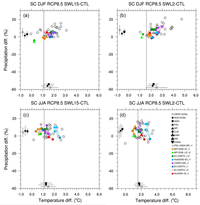
Earth Syst. Dynam., 9, 459–478, 2018 www.earth-syst-dynam.net/9/459/2018/E. Kjellström et al.: European climate change at global mean temperature increases of 1.5 and 2 ◦ C 473 Figure 8. Temperature and precipitation changes over Scandinavia (SC, Fig. 1) for winter (a, b) and summer (c, d) mean conditions. Panels (a, c) show SWL1.5 and (b, d) SWL2. The error bars plotted inside the axis in the diagram illustrate the average and plus or minus 1 SD from (i) the CMIP5 ensemble (Table 2), (ii) the nine-member GCM ensemble that has been downscaled and (iii) the 18-member RCM ensemble (Table 1). Unfilled circles are CMIP5 GCMs listed in Table 2 that have not been downscaled. Filled circles represent GCMs that have been downscaled and these are connected by a line to the RCM(s) that have been used for downscaling. The vertical line represents the global mean warming at SWL1.5 and SWL2 relative to the control period (1971–2000). from www.smhi.se, last access: 10 March 2018), indicating simulated by the underlying GCMs and by the larger CMIP5 a warming of more than 2.5 ◦ C compared to pre-industrial ensemble. However, it is also clear that the range spanned conditions already at SWL1.5. Figure 8 shows that the simu- by the RCM ensemble (or that spanned by the underlying lated future warming is stronger in Scandinavia compared to GCMs) is more limited compared to the full CMIP5 en- the global mean warming already at SWL1.5 and even more semble. Comparing individual simulations reveals that the pronounced at SWL2 for the majority of the simulations. For RCMs do modify the climate change signal from the under- precipitation, the majority of the simulations indicate that it lying GCMs. There are, however, large differences in how will become wetter in both winter and summer, which is al- large these modifications are. For instance, the REMO RCM ready seen at SWL1.5 and more clearly in SWL2 in many only changes the climate change signal from the MPI-ESM- simulations. However, for both seasons there are also simu- LR model marginally in all four cases while all three RCMs lations showing only little change or even decreasing precip- that have downscaled HadGEM2-ES change the results sig- itation. nificantly in summer. In the latter case it is even the ques- It is clear that the spread among the simulations becomes tion of changing sign in the precipitation signal: from a de- larger at SWL2 compared to SWL1.5 in both temperature crease in HadGEM2-ES to an increase in the RCMs. A sim- and precipitation based on the full CMIP5 model ensem- ilar discrepancy between HadGEM2-ES and RCA4 was also ble. We note that the RCM-simulated changes in tempera- found in an RCA4 simulation at 50 km horizontal resolution ture and precipitation mostly lie within the range of those as by Kjellström et al. (2016). They also found wetter condi- www.earth-syst-dynam.net/9/459/2018/ Earth Syst. Dynam., 9, 459–478, 2018
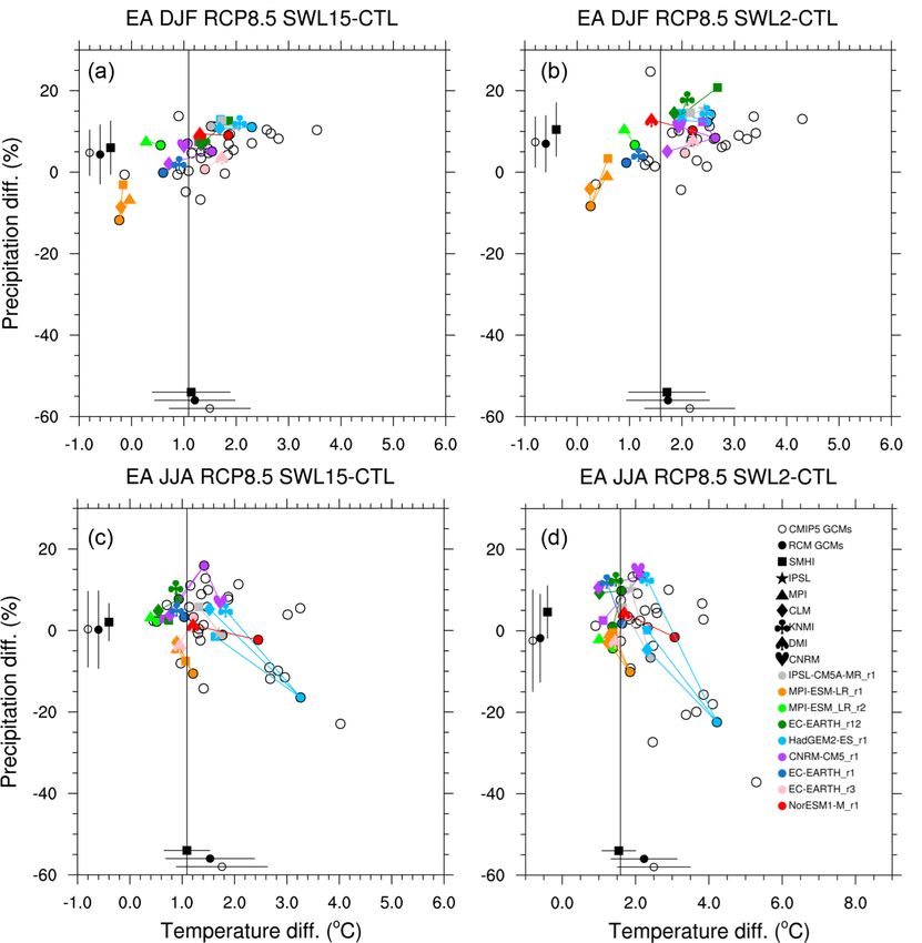
474                    E. Kjellström et al.: European climate change at global mean temperature increases of 1.5 and 2 ◦ C

Figure 9. Temperature and precipitation changes over eastern Europe (EA, Fig. 1) for winter (a, b) and summer (c, d) mean conditions.
Panels (a, c) show SWL1.5 and (b, d) SWL2. The error bars plotted inside the axis in the diagram illustrate the average and plus or minus 1
SD from (i) the CMIP5 ensemble (Table 2), (ii) the nine-member GCM ensemble that has been downscaled and (iii) the 18-member RCM
ensemble (Table 1). Unfilled circles are CMIP5 GCMs listed in Table 2 that have not been downscaled. Filled circles represent GCMs that
have been downscaled and these are connected by a line to the RCM(s) that have been used for downscaling. The vertical line represents the
global mean warming at SWL1.5 and SWL2 relative to the control period (1971–2000).

tions in RCA4 compared to a range of other GCMs it has                     For eastern Europe Fig. 9 shows that simulated changes
downscaled, indicating that the hydrological cycle is more              in temperature are slightly larger in summer than in win-
sensitive to the increasing temperatures in this RCM. It is             ter at both SWLs. Also, the spread is larger in summer as
also noted that HadGEM2-ES has a very strong increase in                a number of models give very strong temperature increases
SSTs over the Baltic Sea, as indicated by the local maxima              (among these are HadGEM2-ES that has been downscaled
in near-surface warming (not shown). Large SST changes in               by the RCMs). For precipitation the simulations reveal an
this region have previously been shown to have a very strong            uncertainty not just in amplitude but also in sign of change
impact on regional climate modelling results (e.g. Kjellström           in both winter and summer, with models indicating either in-
and Ruosteenoja, 2007). As coarse-scale GCMs have a fairly              crease or decrease. The ensemble mean shows a tendency to-
poor representation of the Baltic Sea, care should be taken             wards a drying with less precipitation in summer, especially
when analysing results from these models and preferably                 in SWL2. However, more than half of the GCMs and RCMs
a coupled regional climate model system should be used                  actually show increasing precipitation and it is clear that the
(Kjellström et al., 2005). Apparently, many of the RCM sim-             ensemble average is heavily influenced by a smaller num-
ulations assessed here show larger precipitation increases (or          ber of models with relatively strong decreases. Furthermore,
smaller decreases) compared to the underlying GCMs for                  several of these models also show a strong warming, indicat-
the Scandinavian domain, as also indicated by the ensemble              ing a feedback mechanism including reduced soil moisture.
mean statistics.                                                        As for Scandinavia the spread becomes larger at SWL2 com-

Earth Syst. Dynam., 9, 459–478, 2018                                                         www.earth-syst-dynam.net/9/459/2018/
You can also read