Quality and Price Setting of High-Tech Goods - IZA DP No. 14058 JANUARY 2021 Yuriy Gorodnichenko Oleksandr Talavera Nam Vu - Institute ...

DISCUSSION PAPER SERIES

IZA DP No. 14058

Quality and Price Setting of High-Tech
Goods

Yuriy Gorodnichenko
Oleksandr Talavera
Nam Vu

JANUARY 2021

DISCUSSION PAPER SERIES

IZA DP No. 14058

Quality and Price Setting of High-Tech
Goods

Yuriy Gorodnichenko Nam Vu
University of California-Berkeley and IZA University of Birmingham
Oleksandr Talavera
University of Birmingham

JANUARY 2021

Any opinions expressed in this paper are those of the author(s) and not those of IZA. Research published in this series may
include views on policy, but IZA takes no institutional policy positions. The IZA research network is committed to the IZA
Guiding Principles of Research Integrity.
The IZA Institute of Labor Economics is an independent economic research institute that conducts research in labor economics
and offers evidence-based policy advice on labor market issues. Supported by the Deutsche Post Foundation, IZA runs the
world’s largest network of economists, whose research aims to provide answers to the global labor market challenges of our
time. Our key objective is to build bridges between academic research, policymakers and society.
IZA Discussion Papers often represent preliminary work and are circulated to encourage discussion. Citation of such a paper
should account for its provisional character. A revised version may be available directly from the author.

 ISSN: 2365-9793

 IZA – Institute of Labor Economics
Schaumburg-Lippe-Straße 5–9 Phone: +49-228-3894-0
53113 Bonn, Germany Email: publications@iza.org www.iza.org

IZA DP No. 14058 JANUARY 2021

 ABSTRACT
 Quality and Price Setting of High-Tech
 Goods*
 This paper investigates the link between product quality and price setting for central
 processing units (CPUs). Using thousands of price quotes from a popular price-comparison
 website, we find that market fundamentals, such as the number of sellers, median price,
 share of convenient prices and level of seller stability, are important factors for explaining
 price stickiness and price dispersion. We demonstrate that calculations of price inflation
 require conditioning not only on CPU quality, but also on market fundamentals to ensure
 that CPU attributes are priced correctly. Failing to do so can result in an understatement of
 CPU price deflation in the sample period.

 JEL Classification: E31, L11, L81, L86
 Keywords: price setting, e-commerce, product quality, hedonic pricing,
 inflation

 Corresponding author:
 Yuriy Gorodnichenko
 530 Evans Hall #3880
 Department of Economics
 University of California, Berkeley
 Berkeley, CA 94720-3880
 USA
 E-mail: ygorodni@econ.berkeley.edu

 * Standard disclaimer applies. We thank Tho Pham and Daniel Sichel for their valuable support and comments. We
 are also grateful to participants of Swansea Workshop on Prices and Nowcasting, Scottish Economic Society Annual
 Conference, Royal Economic Society Annual Conference, ESCoE’s Conference on Economic Measurement, Workshop
 on Empirical Macroeconomics, and MMF Annual Conference for valuable comments and discussions. Any remaining
 errors are our own.

1. Introduction

The law of one price is the bedrock of many economic models, but the reality often contradicts
the law: similar (or even identical) goods can be sold at different prices in highly integrated
markets. One may hope that the law of one price may still hold for prices adjusted for quality
differences (“price per performance unit”) and other product attributes. This idea is the basis
of hedonic pricing used to measure inflation for goods with rapid technical change. Indeed,
since Solow (1960), economists and statistical agencies routinely postulate that vintages of
capital produced with different technologies should have the same price when these vintages
are measured in efficiency units. While intuitive, this approach ignores the fact that price
dispersion may arise for other reasons such as market power, price stickiness, and other
frictions. Consequently, conventional hedonic pricing may provide a distorted measure of
inflation.

To evaluate this hypothesis, we use detailed data on price quotes and performance measures
for Central Processing Units (CPUs) to study how quality differences and various frictions
influence measured inflation and technical change. We focus on the CPU market for several
reasons. First, CPUs have a high rate of quality improvement which helps us to explore the
effect of quality changes on prices, as many vintages of CPU technology coexist in a given
period. Second, because CPUs are a key element of many electronic devices, quality
improvement in CPUs is the major factor which contributes to the increase in the quality of
other products and services (desktops, laptops, tablets, mobile phones, software, and cloud
computing); see e.g., Jorgenson et al., 2000; Oliner and Sichel, 2000; Brynjolfsson and Hitt,
2003. Finally, CPU quality can be accurately measured using CPU performance scores, which
removes the difficulty of quality measurement encountered by previous studies (see e.g.,
Combris et al., 1997).

A central ingredient of our analysis is our unique dataset, which includes monthly online prices
of CPUs in the U.S. The online price quotes are collected from a leading online shopping
platform. Our data covers the prices of hundreds of CPUs sold across hundreds of online
retailers between April 2009 and December 2012. The substantial size of our data gives us
strong statistical power. Finally, for each product, we have CPU performance scores, an
integral measure of CPU quality.

Using the dataset, we show that, similar to prices for other products, CPU prices exhibit some
stickiness even in a highly competitive e-commerce environment, thus suggesting that various

 1

pricing frictions and market fundamentals—the number of sellers (a proxy for market
concentration), median price (a proxy for incentives to search for better prices), share of
convenient prices (also called price points such $9.99 or $99)—are also important factors for
explaining price stickiness and price dispersion. We document a variety of stylized facts about
CPU pricing and contrast various pricing moments for CPUs with the corresponding moments
for typical goods sold online. Our results suggest that quality differences play an important role
in accounting for price differences across different CPUs. When we combine market frictions
and quality differences to explain variation in CPU prices, we find that both types of forces are
significant predictors of price variation. Using the introduction of new (sometimes
“breakthrough”) CPU models, we also examine how prices of other models evolve in response
to these technological shocks. We document that the re-pricing of older, less efficient/powerful
models is rather modest and sluggish. Finally, we augment standard hedonic-pricing
regressions to include various measures of market/product fundamentals to investigate how
these fundamentals can affect measured inflation for quality-adjusted products. The estimates
suggest that controlling for market/product fundamentals materially influences estimated
inflation: prices fall at a faster rate than is implied by quality adjustment alone.

Our work is related to several strands of the literature. The first strand studies the micro
foundation of price stickiness (see e.g., Klenow and Malin, 2010 for a survey). Our analysis
complements this strand by focusing on goods with rapid quality improvement and by studying
the effects of well-measured technological changes on price stickiness and price dispersion.

The second strand of literature focuses on price dispersion at the micro-level. Existing papers
often focus on the degree of price dispersion (Lach, 2002; Kaplan et al., 2019; Sheremirov,
2019). Our study contributes to this literature by exploring the impact of product quality on
between- and within-product price dispersion, as well as documenting the dynamic properties
of price dispersion.

Finally, this study is related to the strand of literature that focuses on constructing hedonic price
indices (see e.g., Shiratsuka, 1999; Kryvtsov, 2016; Byrne et al., 2020), especially for
computing devices (e.g., Pakes, 2003; Aizcorbe et al., 2020) and computer components (e.g.,
Byrne et al., 2018). We complement this strand of literature by introducing an improved, direct
measure of product quality for a larger set of CPUs to construct the quality-adjusted price
indices. More importantly, we quantify the contribution of non-technological factors to
correctly measure inflation.

 2

2. Data

2.1. Data collection

We use a comprehensive dataset of CPU price quotes in the U.S. e-commerce market. Each
product is uniquely identified by the manufacturer product number (MPN). For instance, MPN
“BX80601940” uniquely identifies the “Intel Core i7-940 2.93GHz Processor”. Similarly, each
online seller (e.g., Amazon.com, CostCentral.com, Memory4Less.com, NextWarehouse.com)
is uniquely identified. Our online price-quotes are gathered from a leading price comparison
website (PCW) that provides price quotes for the U.S. online market.1 Specifically, at midnight
on the first day of each month, a python script starts to automatically download webpages with
price quotes. After that, we extract MPNs, seller IDs and prices for each CPU-Seller. Price
quotes in our data are “net”, that is, pre taxes and shipping fees. Relative to previous studies
that typically have one year of data or less (e.g., Lünnemann and Wintr, 2011), we have a
longer time series covering 45 months. This feature of our data allows us to better exploit
changes in the quality of CPUs over time.

We complement these price quote data with information on the performance scores of CPUs.
In this additional dataset, we uniquely identify each CPU model by its official name. Besides
performance scores, the data also include the main technical characteristics of the processor
such as speed, turbo speed, and the number of cores. The data of CPU performance scores are
provided by PassMark Software, a leading authority in software/hardware performance
benchmarking and testing. This company is also a Microsoft Partner and Intel Software Partner
and owns one of the world’s largest CPU benchmark websites. They not only report the final
scores of CPU performances but also provide all of the test results used to compute the
performance marks. Furthermore, their testing methods and models to produce the CPU’s
performance score are published on their website. Therefore, if they change their performance
measure, we can produce new performance scores and update our data to be comparable with
new CPU models. Since each CPU model in the latter dataset includes several product versions
with different MPNs in the former dataset, we manually matched the performance score of a
CPU model with all of its versions. For example, the CPU model “Intel Core i7-940 2.93GHz

1
 Gorodnichenko and Talavera (2017) use the same PCW and they provide more details on the prominence and
business model of this PCW.

 3

Processor” has three versions with the same performance. Its MPNs are:
“AT80601000921AA”, “BX80601940”, and “BXC80601940”.

We use performance scores rather than physical characteristics (e.g., clock speed)—as was
done in previous research—because the nature of technical change can evolve over time and
some physical characteristics can lose their relevance. For example, Byrne et al. (2018) find
that the CPU quality index based on chip characteristics is completely flat over 2010-2013,
while the quality index based on performance scores increased sharply. The main reason is that
processor producers shifted away from increasing the clock speed due to heat generation.
Instead, they improved processor performance by placing multiple cores on a chip.2 We
complement existing literature by using the performance score as an integral measure of quality
for a large set of CPUs.

2.2. Data filters and data quality

We applied a series of filters to ensure the consistency of our analysis. Specifically, we dropped
CPUs that do not have performance scores after merging our two data sources. All used or
refurbished CPUs were removed from the dataset since their prices are not comparable with
prices of new CPUs. In addition, to minimize the effects of extreme values in our data, both
the top and the bottom one percent of the prices were dropped. For time-series analyses, CPUs
with less than 20 price-quote observations were removed. A CPU is considered as an available
product in a month if it is offered by at least three sellers in that month. After applying all
filters, our large sample covers monthly prices of 654 CPUs sold across 142 online retailers in
the United States from April 2009 to December 2012. We define an observation by its MPN,
seller ID and month. Our dataset contains 74,306 product-seller-month price quotes. The CPU
market is dominated by Intel and AMD and therefore the price quotes are effectively for these
two manufacturers.3

One may be concerned about the quality of price quotes on PCWs, e.g., the price listed on
PCWs may be out of date or discrepant from sellers’ actual prices if sellers post lower prices
on PCWs than on their websites to attract visits of customers. In fact, online merchants are

2
 Flamm (2019) provides a review of changes in technology.
3
 In the early 2000s, Intel and AMD tended to review their prices quarterly (Goettler and Gordon, 2011). However,
at the end of the decade, the frequency of price reductions of Intel products decreased substantially (Byrne et al.,
2018).

 4

incentivized to keep updating their latest prices on PCWs as they usually have to pay for clicks
on those webpages. Therefore, if their prices are not up to date, they will not gain sales and
will waste their money. Similar to our dataset, Gorodnichenko and Talavera (2017) gathered
price data from PCWs and find that prices on PCWs and seller websites are highly consistent
(correlation 0.98). In addition, they find that price data from PCWs are consistent with the
Bureau of Labour Statistics (BLS) data and are updated rapidly in response to shocks. Hence,
the price data from the PCWs are of a reasonably high quality.

2.3. Notation and aggregation

We use ist to denote the price of CPU i sold by seller at month . Q i denotes the performance
score of CPU i. We denote the set of all CPUs, sellers and time as 1, … , , 1, … , ,
 1, … , . For example, st is the total number of CPUs, which are offered by seller s at
time t, while it represents the total number of sellers that sell CPU i at time t. We will use
lower-case letters to denote logs of corresponding variables; e.g., ≡ log . Bars denote
average values; e.g., ̅ is the average log price of CPU i across all sellers at time t.

We aggregate statistics for a given moment (frequency of price changes, size of price
changes, price dispersion, etc.) as follows:
 ∑ ∑ . (1)

To highlight the differences in the price per unit of performance, we compute the quality-
adjusted price ≡ / where is the median performance score between
all CPU models.

3. Basic facts

This section describes the evolution of the CPU market over the sample period. We will use
institutional details to study how quality improvement affects CPU pricing.

3.1. CPU generations over the last decade

The concept of CPU generations was introduced after Intel released its CPU core i series in
Nehalem microarchitecture family, which is also known as the first generation. The major
difference between CPU generations is the differences in their microarchitecture, which is

 5

reflected by the semiconductor manufacturing process (also called “technology node” or
“process technology”). The “process technology” is designated by the process’s minimum
feature size that is indicated by the size in nanometres. This size refers to the average half-pitch
(half the distance between identical features) of a memory cell (Hoefflinger, 2011). The smaller
the process’s minimum feature size, the more powerful and the more efficient in energy
consumption the processor. Chip companies were able to shrink the size of their
microprocessor and improve the CPU performance, mainly because of the innovation in the
semiconductor industry.

Figure 1 shows that Intel was the pioneer of microprocessor technology in our sample period
from 2009 to 2012. The first generation of the Intel Core processors (Nehalem) was released
in November 2008 and uses the 45 nanometres (nm) process, the second-generation processors
(Sandy Bridge) and the third-generation processors (Ivy Bridge) use 32 nm and 22 nm,
respectively. Meanwhile, AMD was struggling in the technology race with Intel. AMD released
its first-generation CPUs (Bulldozer family) using 32 nm technology 9 months after the release
of the Sandy Bridge processors. The second-generation CPUs of AMD (Piledriver family),
which were released five months after Intel released Ivy Bridge CPUs, were still based on the
32 nm technology.

Table 1 shows that there is variation in performance scores across CPUs within a generation,
because manufacturers can tweak various attributes and features depending on market demand.
As a result, CPUs in a later generation are not always better than CPUs from earlier generations.
However, newer generations do tend to have better performance on average. For example,
CPUs in the Nehalem generation have, on average, more than 100% improvement in
performance scores relative to older CPUs. CPUs in the Ivy Bridge generation have, on average,
30% higher scores than CPUs in the Nehalem and Sandy Bridge generations, but the Sandy
Bridge generation was roughly comparable to the Nehalem family. On average, a new
generation improves performance scores on the order of 50%.

Panel A of Figure 2 shows the number of CPU models of each generation over time following
a new CPU generation release. The number of available new generation CPU models gradually
increases, while old generation CPU models leave the market. It implies that processor
producers do not release all models of a generation when they introduce new technology.
Instead, they often release a few new models first, then launch more models using that new
microarchitecture and stop selling old generation products.

 6

To adopt the technological upgrades in the market from processor manufacturers and consumer
demand, sellers respond by updating the list of CPUs that they are offering. Panels B and C of
Figure 2 clearly show a rapid increase in the number of sellers that offer new generation
processors and in the number of new-generation models offered by a seller, respectively. As a
result, the number of observations of new technology CPUs dramatically rose after their
releases. These facts suggest that the change in performance scores of CPUs offered by sellers,
which is caused by the entry of new CPUs and the exit of old CPUs, should be able to reflect
the technological upgrades in the market.

3.2. Price distribution and performance

Table 2 shows the average price of each percentile of the distribution over products ( ), the
mean and the standard deviation of the average log price ( ̅ ) within the sample. Overall, the
median CPU in our data costs $190.43 and 25% of the CPUs are priced under $99.95; CPUs
that are more expensive than $334.93 account for the top 25% of highest prices of the sample.
When we adjust prices for performance scores, we observe that price dispersion (measured as
the standard deviation of log prices) falls by 6 log points from 0.90 to 0.84.

To further explore the relationship between prices and performance, we compute log deviations
for prices and performance scores from the median CPU in a given month and present a
binscatter plot in Figure 3. Each bin (point in the figure) corresponds to one percent of the
sample. The lowess smoother (bandwidth set to 0.1) plots the non-parametric fit. The figure
shows that better-performing CPUs command higher prices. However, the relationship is non-
linear (concave) as the curve is flatter on the right-hand side of the price distribution,
demonstrating that consumers have to spend increasingly more money to achieve a given gain
in performance.

To compare the price per performance unit of CPUs in different quality standards or price
levels, we divide our sample into four quartile groups of CPUs based on their performance
scores. Panel A of Figure 4 shows the distribution of average CPU prices by quartile. The
estimated kernel densities suggest that high-performance CPUs are sold at higher prices and
the peaks of estimated densities are shifted to the right as we move from the first performance
quartile (lowest performance) to the fourth performance quartile (highest performance). Panel
B of Figure 4 shows the corresponding distribution of CPU prices adjusted for quality, i.e., the

 7

average price per performance unit of CPUs ( ). Note that the distance between
distributions is discernibly attenuated and therefore some (but not all) of the observed price
dispersion is accounted for by differences in CPU productivity.

Finally, we split our sample by CPU generation (described in the previous section). Panel C of
Figure 4 presents the distribution of average prices within a CPU generation, while Panel D
presents the corresponding results for quality-adjusted prices . The price per unit of
performance for AMD processors was generally lower than the price for Intel processors. This
discount could reflect the fact that AMD was often catching up with Intel and thus AMD had
to offer discounts to compete with the dominance of Intel in the CPU market (see e.g., Goettler
and Gordon, 2011). In addition, we observe that the technical improvement used in later CPU
generations benefits customers by reducing the price per unit of performance. However, the
difference in the average price per performance unit between a CPU generation and its next-
generation is usually small.

3.3. Dynamics of CPU prices

Panel A of Figure 5 shows that the price level in the CPU market ( ) slightly increased as the
new-generation CPUs were released at higher prices, but the quality-adjusted prices ( )
dropped quickly due to the significant improvement in CPU performance, which is consistent
with earlier studies (e.g., Byrne et al., 2017; Byrne et al., 2018).

Panel B of Figure 5 illustrates the dynamics of the median price of each generation. The median
prices of AMD generations were often lower than prices for Intel counterparts. We also see
that CPU producers usually set higher prices for new generation processors and the median
prices tend to gradually decrease over time.4 However, the median prices of Intel Core 2 and
Intel Nehalem CPUs were consistently higher than the median prices of new generations and
remained stable for most of our sample period. This can be explained by the large demand for
those two processor generations in our sample period. Since those old CPUs were popular for
a long time without major changes to the processor architecture, the old systems, which are not
compatible with new processor generations, were also popular. Thus, a large number of
customers might choose to purchase an old-generation processor rather than upgrading the

4
 Nehalem prices dropped sharply in early 2010 when Intel introduced a new model in the Nehalem family.

 8

whole system, while the supply of these old models is limited as Intel stopped producing them.
This could lead to a high price level of Core 2 and Nehalem CPUs.5 We observe similar patterns
when we examine the dynamics of prices adjusted for quality (Panel C of Figure 5).

4. Pricing facts for CPU e-commerce

In this section, we document the basic facts about price setting for CPUs in the online retail
market. Specifically, we focus on the frequency of price changes, size of price changes, and
within-CPU price dispersion. To compute these moments, we follow Gorodnichenko,
Sheremirov and Talavera (2018) and provide pertinent definitions and notation in Appendix B.
We then relate each of these moments to market fundamentals and contrast these moments with
the corresponding moments for typical goods sold online, which generally have a lower rate of
technical change. Note that one should expect to find smaller pricing frictions in online markets
than in conventional “bricks-and-mortar” markets because e-commerce has small nominal
price change costs (“menu costs”), small search costs, and small costs of monitoring
competitors’ prices (Ellison and Ellison, 2005).6 Thus, online price quotes increase our chances
of detecting the rapid repricing of CPU models in response to technological advances.

4.1. Frequency and size of price changes

Following previous studies, we determine the frequency of price adjustment as the proportion
of non-zero price changes to the total number of price changes observed within our dataset
(e.g., Bils and Klenow, 2004; Klenow and Kryvtsov, 2008; Nakamura and Steinsson, 2008;
Eichenbaum et al., 2011). Specifically, we consider a price change that is smaller than 0.1% as
a zero-price change, that is, the price is treated as fixed if the deviation from the price in the
previous month is very small.

Table 3 reports that the median of the frequency of regular price adjustments is 39.4% per
month (that is, 39.4% of prices are changed from one month to the next) and the implied

5
 CPU producers changed their life-cycle pricing strategy and stopped reducing the price of old models.
6
 Because we do not have sales flag as in scanner data, we follow previous studies (e.g., Chahrour, 2011) to
identify temporary sales with a “sales filter”, which is the ˅-shape or ˄-shape in price changes. Specifically, we
consider an increase or decrease in price as temporary price changes if the price returns to its previous price level
within one month. The mean frequency of sales across CPUs is 1.88% and the median size of sales across CPUs
is 2.28%. Because sales are not prevalent for CPUs, we report statistics only for “regular” prices (that is, prices
without sales) to preserve space. Moments for posted prices (that is, prices with sales) are available upon request.

 9

duration of a typical price spell is two months.7 These moments are broadly similar to what can
be observed for a representative basket of goods sold online. However, in contrast to typical
goods in e-commerce, CPUs have a more pronounced bias towards price decreases relative to
price increases. Specifically, the frequency of price decreases is 22.4% per month for CPUs
and 15.6% per month for a typical product sold online. Meanwhile, the corresponding figures
for price increases are 15.2% and 13.9%. This pattern is consistent with a faster technical
change in the CPU market which forces CPU sellers to mark down their prices more often.

We observe a similar pattern for the average absolute log price change (| |). The average
change for all price adjustments is similar for CPUs (8.1%) and typical goods (10.9%) but there
is a clear asymmetry in the size once we condition on the direction of price change. The average
size of price decreases for CPUs is 9.2% while the average size of price increases is only 5.6%.
In contrast, the size of price changes for typical goods is roughly symmetric: 11.8% for price
increases and 10.3% for price decreases.

More generally, these results suggest that, relative to the conventional markets, the frequency
of price changes is high and the size of typical price changes is small—facts consistent with
easy/cheap nominal price adjustment—however there remains discernible price stickiness
which can be rationalized by market/product characteristics. To further explore this conjecture,
we regress pricing moments on six variables: (1) number of sellers that sell product i; (2) quality
of product i; (3) the median price of product i; (4) share of price points, which is the percentage
of price quotes that end at 9, 95 or 99 for product i (e.g., $199, $349, $495); (5) the stability of
sellers for product i is the ratio of the number of sellers offering product i in a given month to
the number of sellers ever selling this product in the quarter, which covers the given month;
and (6) CPU producer, which is a dummy variable that equals 1 if it is an Intel CPU and equals
zero otherwise. The first variable proxies for market competition (e.g., Ginsburgh and Michel,
1988; Martin, 1993). The second variable captures the characteristics of goods. The third is a
proxy for the returns of buyers’ searches (e.g., Head et al., 2010). The fourth reflects the level
of inattention to prices when choosing between products (e.g., Knotek, 2011). The fifth variable
(stability of sellers) is a proxy for the turnover of sellers (e.g., Gust, Leduc, and Vigfusson,
2010). The last variable aims to capture the special role of Intel in this CPU market.

7
 If ̅ is the average frequency of price adjustment for CPU , the mean implied duration is given by ̅
 log 1 ̅ .

 10

Table 4 reports the results of regression for the frequency and size of price adjustments as
outcome variables. All variables are measured at the product level. For instance, the frequency
of price changes at the product-level for a specific product is computed as follows: First, the
frequency of price adjustments for each seller offering that product is calculated. Then, the data
is collapsed to product-level by taking the raw average across sellers to use as a dependent
variable and the regression is estimated with no weights.

We find that all explanatory variables have some predictive power. First, a market with more
sellers should have a higher (lower) frequency of positive (negative) price changes, and a
smaller size of adjustment. Second, the quality of goods in the market is positively associated
with the degree of price flexibility (higher frequency and smaller size of price adjustments).
This is because a high-quality product often has lower search costs due to higher advertising
expenses and higher returns on searches for customers.8 We also find that a more powerful
processor has price increases less often and price decreases more often. This can be explained
by the observed quality premium, which provides more room for sellers to adjust prices. Third,
for products with low- and moderate-prices, price changes occur more often and are larger in
size when the median price across sellers of a product increases. This result is consistent with
Head et al. (2010), documenting that higher returns on searches would put more pressure on
the seller to adjust prices. Nevertheless, given the estimated nonlinearity, very expensive CPUs
tend to have fewer and smaller price changes. Fourth, a product which has a high proportion
of price points has a lower frequency of price changes, particularly positive price changes. This
result is consistent with Levy et al. (2011), who find that prices ending with 9 have a lower
frequency of price changes. Fifth, an increase in the degree of seller stability, which implies
that it is more difficult for new sellers to enter the market, is associated with a decrease in the
frequency of price changes, particularly, the frequency of negative price changes. Lastly, Intel
processors tend to change prices more frequently than AMD products.

4.2. Price dispersion across sellers

Hedonic pricing of different vintages largely focuses on explaining variations in prices across
vintages, rather than within-vintage price dispersion. However, price dispersion across sellers
within a product can help us to directly measure potential “mispricing” and frictions in the

8
 For the negative relationship between customer search and price stickiness level, see i.e., Ellison and Ellison
(2009).

 11

market because the quality of the product is held constant. Indeed, if there is dramatic within-
product price dispersion, one may be less sanguine about using hedonic regressions to price
properties of products since the market does not eliminate arbitrage opportunities.

4.2.1. Intra-month dispersion across sellers

We use several measures of within-CPU price dispersion, which capture different aspects of
price variation: the coefficient of variation (CV; the ratio of standard deviation to the mean),
standard deviation of the monthly log prices, the log difference of the average and the lowest
price (the value of information (VI)), interquartile range (IQR), range (the log difference
between the lowest and highest price), and gap (the difference between the two lowest log
prices). We calculate the measure of price dispersion between sellers for an identified CPU in
a month, then collapse our data to product level by taking the raw average over time.

One might argue that the observed price dispersion is caused by the differences in the shopping
experience that customers have with different sellers (see e.g., Stigler, 1961). This difference
is not likely to be significant when customers are shopping online as consumers only deal
directly with a seller after completing the transaction. To further alleviate this potential
problem, we purge “shopping experience” from prices using the following regression:
 (2)
where and control for product and seller fixed effects, respectively. The fixed effects can
capture the differences in reputation, delivery conditions, and return costs between CPU
retailers. Thus, the dispersion of the residuals gives us the price dispersion net of sellers’
heterogeneity in, for example, shipping costs and return policies, which are likely to remain
unchanged over a short period of time (see e.g., Nakamura and Steinsson, 2008).

We report price dispersion for and in Panel A of Table 5. CV (row 1) for is 0.22,
thus suggesting considerable heterogeneity in prices, even for a fixed CPU. The standard
deviation of log prices (row 2) is also relatively high at 0.23. Seller fixed effects account for
around 20% of the variation in actual CPU prices in the U.S. online market (see row (7)) and
the residual price dispersion is 0.18. The within-product dispersion for CPUs is generally
similar to the within-product dispersion for goods typically sold online (column 2 of the Table).

 12

4.2.2. Price dispersion across sellers over CPU lifetime

The price dispersion across sellers of a product may depend on the stage of the product lifetime.
Dispersion is expected to be higher at the release time of a product and then gradually decreases
as customers increase their awareness of the pricing strategy of sellers and sellers collect
information about their competitors’ prices. In a stationary setting (i.e., the set of products is
fixed), lifetime price dispersion is not important. However, when there is a turnover of
products, one may observe the dispersion of prices in a cross-section simply because we have
a mix of “new” products that have large price dispersion and “old” products that have low price
dispersion. If price dispersion declines over the lifetime of a product, one may expect that
hedonic pricing of attributes works well because the law of one price may hold for established
products.

To study this aspect of price dispersion, we calculate the average price dispersion across CPUs
for month j after their introduction. Following Gorodnichenko et al. (2018), we identify the
time of product introduction by taking the time that the product appeared in the data. CPUs
which enter within the first quarter are excluded, as we cannot know whether the CPU was
released previously or it returned after being temporarily unavailable. Following this, the
measure of price dispersion over a CPU lifetime is computed as follows: We generate the time
variable for each processor as the number of months since the month that the processor
appeared in the dataset to replace the calendar months. Then we use the cross-sectional price
dispersion of each processor and the new time variable to compute the average price dispersion
across CPUs for j month after their release month.

We find little evidence of price convergence across sellers offering a CPU over the product
lifetime. Figure 6 shows that, since the time that a product is released, price dispersion increases
slowly over the first two years from around 0.14 to nearly 0.20. This dynamic is likely to be
explained by evolution in the depth of the market, because the number of sellers stays relatively
constant over a product’s lifetime. Interestingly, price dispersion also increases over the
lifetime of goods typically sold online but the profile of the increase is flatter.

4.2.3. Spatial vs. temporal price dispersion

Understanding the nature of price dispersion can show us how persistent mispricing can be, as
well as how one can select outlets to correctly price product attributes. The existing literature

 13

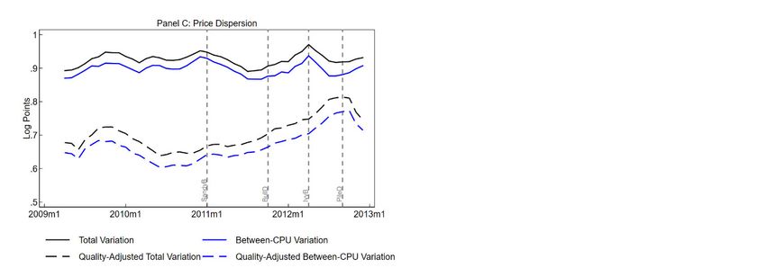
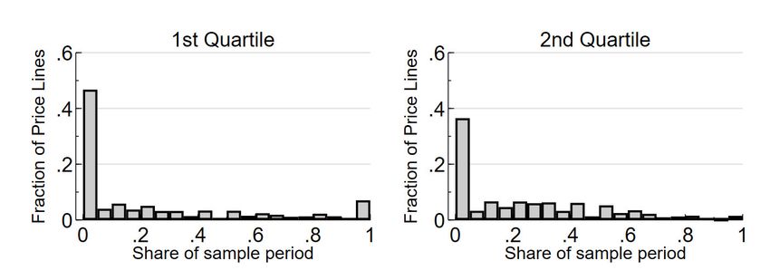
on price dispersion posits two main types of price dispersion: spatial and temporal. Spatial
dispersion refers to the situation in which some sellers persistently charge higher prices for
their product because they have, for example, a better location (see e.g., Baye et al., 2010). In
contrast, temporal dispersion refers to the situation in which sellers do not consistently charge
lower/higher prices for their product because over time buyers learn sellers’ pricing behaviour
and identify the seller who offers the best price (see e.g., Varian, 1980; Sheremirov, 2019).
Appendix Table A4 provides examples for spatial and temporal price dispersion. The form of
price dispersion affects whether or not one can use outlets for sampling prices interchangeably.
Specifically, if price dispersion is temporal, the identity of the seller is less important because
one can recover the average price in the market by following this seller. In contrast, if price
dispersion is spatial, the identity of the seller is important for measuring the level of prices in
the market.

Following the method developed by Lach (2002), we assign the price of a product offered by
a seller (“price line”) to a quartile of the price distribution across all sellers of that product in a
given month, then analyze movements across quartiles of that price line over time. For
example, the price of retailer s for CPU i in month t is and three cut-off points for product
i in month t are , , . Then, a seller with the price for product i such that 

 is in the second quartile of the cross-sectional distribution in month t, while a seller

with the price is in the fourth quartile (i.e., the price for CPU i is higher than 75%
of prices offered by all sellers for CPU i in month t). Following this step, we construct the
fraction of time that spends in each quartile and the average fractions across CPUs.

If sellers do not consistently set their price lower/higher than prices of other sellers and instead
charge high prices at times and low prices at other times (i.e., temporal price dispersion), the
probability of a given price line remaining in each quartile of the price distribution should be
similar and near to 25%. If sellers consistently charge lower or higher prices (i.e., spatial
dispersion), would spend more time in one of the quartiles. We find evidence consistent
with spatial price dispersion in our data.9 Rows (12)-(15) of Panel B in Table 5 show that 20.9%
of price lines spend more than 95% of the time in one quartile of the cross-sectional
distribution. Furthermore, 9.8% of price lines almost always stay in the lowest quartile and
7.3% of price lines almost always stay in the highest quartile. In addition, rows (8)-(11) in the

9
 Because the results for “raw” prices and residual prices (i.e., , prices net of seller fixed effects) are similar,
we only reported results using “raw” prices.

 14

table show that from 37.2% to 50.1% of price lines spend almost no time in a given quartile.
For example, 42.6% of price lines rarely stay in the cheapest quartile and 50.1% of price lines
rarely stay in the most expensive quartile.10 These results are broadly similar to the
corresponding moments for a representative basket of goods sold online (column 2).

The last row in Table 5 presents another useful metric: the average standard deviation across
price lines of the fractions of time spent in a particular quartile. The average standard deviation
equal to 0 implies perfect temporal price dispersion, while the value of √3⁄4 ( 0.43) implies
perfect spatial price dispersion. In fact, the average standard deviation is 0.29, which is closer
to 0.43. For comparison, this metric stands at 0.31 for a typical product sold online.

4.2.4. Predictors of within-product price dispersion

Economists generally rationalize price dispersion with three forces: search costs, price
stickiness, and price discrimination.11 To assess the role of these forces to explain within-
product price dispersion for CPUs, we estimate the following regression:

 log (3)

where is the average of monthly within-CPU standard deviation of the log prices for CPU ,
 is the performance score of CPU , is a vector of market/product characteristics of CPU i
such as the average number of sellers for CPU , share of price points (proportion of pricing
points ending with 9 or 95-99), stability of sellers’ pool, Intel indicator variable, and price
stickiness measures (frequency and size of price changes).

Table 6 reports the results for the regression of standard deviation of log price in column (1).
We find that CPU performance is negatively correlated with price dispersion. On the other
hand, median price, frequency and size of regular price adjustments are positively associated
with price dispersion. The results are similar between the regression of posted prices and
residual prices after removing seller fixed effects (column 2).

4.3. Taking stock

10
 Furthermore, Appendix Figure A1 plots the distribution of these fractions over observed price lines to provide
a clear picture of the existence of the spatial dispersion.
11
 See Gorodnichenko, Sheremirov and Talavera (2018) for a discussion.

 15

Our results suggest that price setting in the online market for CPUs is consistent with
discernible frictions due to price stickiness and market structure. While there are clear signs of
fast technical change in CPU prices (e.g., price decreases are larger and more frequent than
price increases), CPU prices tend to have spells as long as spells for other goods sold online,
despite the fact that CPUs have faster technical change than many other goods sold online.
Within-product price dispersion tends to have properties largely similar to those for a typical
product in e-commerce: dispersion is large and “spatial”. Furthermore, price dispersion and
stickiness can be explained by market structure (e.g., number of sellers) and product
characteristics (e.g., product prices which influence incentives to search for better prices).
These facts point to two important observations. First, market/pricing frictions can materially
affect price differentials across CPUs. Second, the selection of outlets may be important for
the quality of hedonic calculations, that is, price quotes from some outlets may result in
overstating (or understating) the value of attributes and hence distort estimates of inflation in
prices adjusted for quality differences.

5. Technological changes and CPU pricing

Previous sections document that CPU pricing depends not only on CPU performance but also
on a variety of market fundamentals.12 Furthermore, the pricing of CPU performance can vary
with market/product characteristics. In other words, we may be unable to use CPU-A’s price
to benchmark CPU-B’s price by performance alone because the unit of performance may be
priced differently for CPUs A and B due to differences in market power, price stickiness, etc.
As a result, when CPU prices are compared, we need to hold constant, not only CPU
performance, but also market structure.

To build intution for this point, let us suppose we need to compare an exiting CPU model (call
it CPU A) in period to an entering CPU model (call it CPU B) in period 1. The prices for
A and B may be different because B is more powerful than A or because the seller (or producer)
of A has a different market power relative to the seller of B. To have the correct measure of
inflation, we need to take two actions. First, we need to construct the price that the seller of A
would have charged if it sold B. Once this price is constructed we can adjust that price for
quality differences between A and B. The hedonic regressions adjust for the second step of this

12
 With a slight abuse of terminology, we equate markets with products. In other words, the set of sellers for a
given product is treated as a market.

 16

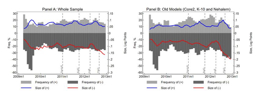
process, but they do not adjust for the first step of the process because they implicitly assume
that sellers are interchangeable (e.g., the law of one price holds).

In this section, we investigate how between-CPU price dispersion can be rationalized by
differences in CPU performance, as well as market fundamentals. To this end, we first examine
the evolution of CPU prices in response to the introduction of new CPU models. We then
attempt to predict average CPU prices (across sellers) in a regression context. Finally, we use
hedonic regressions to estimate inflation for CPUs, holding performance and market
fundamentals constant.

5.1. Pricing moments and technology shocks

As discussed above, there were several breakthroughs in CPU technology: January 2011 when
Intel introduced Sandy Bridge CPUs (the second generation of Intel Core processors) using 32
nm technology nodes; October 2011 when AMD released Bulldozer family 15h (the first
generation) using its 32 nm process technology; April 2012 when Ivy Bridge processors (the
third generation of the Intel Core processors; the 22 nm process) were released, September
2012 when AMD released Piledriver family 15h (the second generation, which had some
improvements but still used the same module 32-nm design with Bulldozer). One may expect
major re-pricing of CPUs around the time when new generations become available. Indeed, if
a new generation of processors improves performance by 50% on average, prices for existing
models could decline by as much as 50%.

Panel A and B of Figure 7 illustrate the monthly frequency and average absolute size of positive
and negative price adjustments throughout these shocks. Panel A of the figure uses the full
sample, while Panel B uses the data that is restricted to the older generations (namely AMD
K10, Intel Core 2, and Intel Nehalem). The release of a new CPU generation generally
decreases the frequency and size of positive price changes and increases the frequency and size
of negative price changes (Panel A). These effects are more visible for older CPUs (Panel B).
However, it is clear that these price changes fall short of a major (50% or so) repricing for
existing CPUs. Furthermore, price adjustment is gradual in the data, while theory predicts
instantaneous adjustment.

Panel C of Figure 7 paints a similar picture: the introduction of new technologies does not lead
to large, rapid changes in the distribution of prices for existing CPUs. For example, the

 17

dispersion of CPU prices in a given month stays roughly constant, irrespective of whether we
look at the total price variation (i.e., between-product and within-product variation; black line
in the figures) or between-CPU price variation (blue line) or whether we use raw prices (solid
line) or quality-adjusted prices (dashed line).

5.2. Predictors of between-product price variation

Hedonic pricing implicitly assumes that the only systematic source of price differences across
goods (“vintages”) are attributes that are valuable to consumers (e.g., processor clock speed,
energy consumption, etc.). Our analysis of within-product price variation suggests that
market/product characteristics can account for some part of price differentials across sellers for
a given product, that is, if the quality of the product is held fixed. These findings suggest that
pricing of product attributes can also depend on market fundamentals. If this is indeed the case,
then hedonic pricing may provide a distorted assessment of what portion of price variation is
due to changes in attributes and what portion is purely due to inflation. Intuitively, if attributes
are priced differently across two markets (CPUs), we should be cautious when using one of the
markets to price goods in the other market. Specifically, to compute inflation, we should hold
constant, not only product attributes, but also market fundamentals (that is, the pricing scheme
for the attributes).

To explore the quantitative importance of this point, we estimate the following regression:

 ̅ log log (3)

where ̅ is the average price (across sellers) of CPU in month , is the performance score
of CPU , is a vector of market/product characteristics such as a CPU’s market concentration,
average price (proxy for returns on search), price stickiness, stability of sellers, share of price
points and product brand. Coefficient measures the sensitivity of CPU prices to its
performance. Coefficient vector may be interpreted as measuring markups and other
distortions in the market for a given CPU. Coefficient vector captures differences in pricing
of the relevant attribute (here the performance scores) across markets (i.e. how a given market
characteristic alters the price of the attribute). Standard hedonic regressions impose 0 and
often 0. Note that while the quality (performance) of a CPU is fixed when the CPU is
introduced, market fundamentals can evolve as we can have, for example, the entry or exit of
sellers.

 18

We find (column (1) of Table 7) that the elasticity of CPU price with respect to its performance
score is 0.5 and performance alone can account for approximately 30% of the variation in prices
across CPU models. Market characteristics (column (2)) are also statistically significant
predictors of CPU prices, but these predictors can account for only 6.3% of price variation and
the interpretation of estimated coefficients can be counterintuitive (e.g., as the number of sellers
increases (more competition), CPU prices increase), which underscores the predictive rather
than causal nature of specification (3). Once we condition on CPU quality and market
characteristics (column (3)), the counterintuitive estimates are not an issue. For example,
increased competition (more sellers, less stable pool of sellers) is associated with lower prices.
Notice that the elasticity of CPU prices with respect to performance increases to 0.6. It can also
be seen that Intel appears to charge a 48% premium over AMD. The R2 of the fitted model
increases to 0.39.

Finally, column (4) reports the results when we allow for the interaction of CPU performance
and market fundamentals. All interactions are statistically significant and this further improves
the fit of the model (R2 increases to 0.41). The economic intuition underlying the estimated
coefficients is also potentially of interest. For example, the positive estimate of the interaction
of performance and Intel dummy suggests that Intel can charge higher prices for high-
performance CPUs, i.e., the segment of the market where Intel likely faces less competition
from AMD. These results suggest that the comparison of prices for different technologies
should involve, not only physical properties of the compared technologies, but also the
characteristics of the markets in which these technologies are priced.

5.3. Adjustment of prices following technology shocks

The previous section documents that product attributes and market fundamentals are important
for pricing CPUs. However, specification (3) does not allow us to assess how quickly CPUs
are repriced in response to the entry of new models or the exit of old models. One may expect
that an entry for a new, more powerful CPU should lead to price cuts for existing CPU models,
but how quickly these cuts happen depends on a number of elements, such as how competitive
the markets are and how sticky prices are. To formally explore this insight, we estimate the
following specification:

 19

 (4)

where is a pricing moment for CPU in month (frequency of price changes across sellers
of CPU in month , size of price changes across sellers of CPU in month ), is a vector of
market characteristics and are CPU fixed effects. Indicator variable “Upgrade” equals one
if the product i jumps to a higher performance quartile at time t compared to time 1 and
equals zero otherwise. For instance, when the number of products entering the market with
lower performance scores than product i and/or the number of products exiting the market with
better quality than the product i are sufficient, the product i will jump to a higher quality
quartile. Indicator variable “Downgrade” equals one if the product i falls to a lower
performance quartile at time t compared to the previous period and zero otherwise. We report
estimated coefficients in Table 8.13

Consistent with time-series evidence presented in section 5.1, we find that upgrading or
downgrading a given CPU relative to other CPUs available in the market changes the
probability and size of a price change only marginally. For example, coefficients on
Upgrade/Downgrade separately and coefficients on interactions with product/market
characteristics are generally not significant statistically.

The estimated insensitivity of CPU prices to changes in relative performance position is
consistent with several explanations. First, prices may be very sticky and so they exhibit little
response to the introduction of new models. Given how quickly online prices change, this
hypothesis alone should not be able to account for the observed insensitivity.

Second, new models are priced in such a way that the price of a new CPU does not disrupt the
pricing of existing models. For example, if the price per performance unit is fixed, a more
powerful model can command a higher absolute price, but it would not mean that existing
models are mispriced because they charge the same quality-adjusted price. As discussed above,
even when we compare CPU prices per performance unit, there remains considerable price
dispersion and performance alone accounts for only 30% of the observed price variation across
CPUs. Thus, this hypothesis is also unlikely to be the exclusive explanation.

Third, CPU manufacturers may segment CPU markets. For example, two average CPUs may
not be combined to produce one powerful CPU. In a similar spirit, new CPUs may be
incompatible with other equipment (e.g., motherboards) thus limiting substitutability of CPUs.

13
 Results for alternative specifications are reported in Appendix Tables 2 and 3.

 20

AMD and Intel processors are not fully compatible either. Furthermore, chip manufactures may
require retail sellers to enforce differential pricings so that AMD/Intel can maximize profits.
Such market segmentation can thus limit arbitrage and create potential mispricing (i.e., quality-
adjusted prices will not be the same across CPUs). Consistent with this hypothesis, we observe
that Intel charges systematically higher prices.

Finally, when a new model (or technology) is released, there could be some uncertainty about
the quality of the new release and sellers may be reluctant to re-price “old and tried” models
before new releases are thoroughly benchmarked. This demonstrates why benchmarking firms
such as Passmark have experienced a high level of success. While we cannot test this
hypothesis directly, we conjecture that uncertainty should be dispelled relatively quickly and
therefore this hypothesis is unlikely to be a major factor.

In any case, our evidence is consistent with considerable pricing frictions that can limit the
consistent pricing of CPU attributes across markets, thus posing a potential threat to hedonic
pricing of CPUs.

6. Inflation in CPU prices

Quality improvement has long been a major challenge for measuring inflation, especially for
goods with rapid technological advancements. Hedonic regression is a popular approach for
ensuring the correct prices for upgrades of product attribute trends (see e.g., Gordon and
Griliches, 1997; Shiratsuka, 1999; Bils, 2009). However, this approach ignores the fact that
prices are also affected by other factors, such as market and product characteristics.14

We follow the common approach in the existing literature (see e.g., Byrne et al., 2018; Aizcorbe
et al., 2020) and run the hedonic regression for each pair of consecutive years in our sample.
More specifically, we include product characteristics and market fundamentals as control
variables. Our focus is on the quality-adjusted price movement which is reflected by the
coefficient of the year dummy for each time period. We show that hedonic adjustment may be
incomplete if pricing of product attributes varies across products. Thus, one should control, not
only for product attributes, but also for market fundamentals.

14
 For a related issue in the context of international economics, see e.g., Mallick and Marques (2016) for the
impact of income level in importers’ and exporters’ countries as well as product quality on export prices.

 21

To assess how market fundamentals can affect measures of CPU price inflation, we estimate
the following specification for each pair of consecutive years (i.e., 2009-2010, 2010-
2011, 2011-2012}) in our sample:

 ̅ log log (5)

where ̅ is average price of CPU observed in month , is a dummy variable that equals
1 if the observation is in the 2nd year of the 2-year period. Vector includes market
fundamentals such as (the median price across sellers), (number of sellers) and 
(seller stability), and (an indicator variable equal to 1 if processor is produced by Intel).
Note that we allow coefficients to vary for each two-year sample . We run the regression at
the product-month level. Table 9 reports for various which measure inflation in CPU
prices from one year to the next.

When we do not control for product quality or market fundamentals (column 1), we find that
inflation was ≈25% in 2010 followed by mild deflation in 2011 and 2012. However, rising
prices could largely reflect rapid improvement in CPU performance. Indeed, after controlling
for performance scores (column 2), the price of CPUs (i.e., quality-adjusted prices) fall by just
over 4% in 2010 and by another 11.4% in 2011, but increased by 5.2% in 2012. The cumulative
deflation over the sample period is 10.4%. Controlling for changes in the market structure alone
(column 3) is not enough to capture quality improvements and implied inflation could be in
double digits. Controlling for product quality and market fundamentals, column 4 demonstrates
inflation estimates similar to those when we control only for quality (column 2) but the
magnitudes and timing of inflation are different. For example, measured inflation in 2010 is
3.7% while the timing of deflation is 10.6% in 2011 and 4.3% in 2012. As a result, the
cumulative deflation is only 11.2%. Finally, when we allow for the interaction of market
fundamentals and product quality (that is, for differences in how CPU performance scores are
priced across markets), we find that cumulative deflation is 16.2% which is considerably larger
than the deflation estimated with quality adjustment alone. It should also be noted that the
profile of inflation dynamics is steeper than in column (2).

These estimates suggest that conventional hedonic regressions may provide distorted estimates
of inflation, because these regressions do not control for changes in market fundamentals or
take into account how pricing of product attributes can vary across markets.

 22