A MULTI-SPEED HOUSING MARKET
←
→
Page content transcription
If your browser does not render page correctly, please read the page content below
A MULTI-SPEED
HOUSING MARKET

Niels Arne Dam, Tina Saaby Hvolbøl and Morten
Hedegaard Rasmussen, Economics

INTRODUCTION AND SUMMARY                                   being accompanied by a faster pace of income
                                                           growth, the higher level of house prices could be
At the national level, Danish house prices are in-         temporary, resulting in substantial capital losses
creasing, but the housing market as a whole is still       for households and higher loan-to-value, LTV, rati-
struggling with low turnover, a substantial hou-           os. This places demands on homeowners’ financial
sing supply and a long time on the market. Howe-           robustness. Against this backdrop, it is important
ver, there are considerable regional differences.          for homeowners to build up home equity over
   Large Danish towns and cities, especially               time, thus moving away from the maximum LTV
Copenhagen, are experiencing a surge in house              ratio.
prices, reasonable turnover and limited supply. In            A reduction of the maximum LTV ratio for defer-
recent years, population numbers in large Danish           red amortisation loans could increase the financial
towns and cities have been growing faster than             robustness of homeowners, while at the same
the housing supply, indicating pressure on the             time preserving the security of mortgage bonds.
housing market.                                            This will ensure that the system is robust – even in
   At the same time, prices in most of Denmark             periods of falling house prices. Calculations in this
are unchanged or slightly higher, implying that            article show that reducing the maximum LTV ratio
the market is sluggish with slow trading activity          for deferred amortisation loans from 80 to, say,
and many homes on the market. In some areas,               60 per cent would cause house prices to increase
house prices are falling, and sales are few and far        less than would otherwise be the case.
between. These areas also have an overrepresen-               Housing market stability is also challenged by
tation of enforced sales. Moreover, population             economic policy framework conditions for the
numbers are declining, and there are no immedi-            housing market, which are, in some respects, pre-
ate indications that this will change. If the balance      venting the free formation of prices and leading
between supply and demand is to be restored,               to randomness and inefficiency in the housing
permanent changes in the housing supply are                market. The freeze on property value tax means
required. This will take many years to accomplish.         that this tax is the cause of greater housing price
   The housing market is of great significance             fluctuations. Restoring the link between property
to both financial and macroeconomic stability.             value tax and house prices would help to stabilise
Looking forward, a more stable housing market              prices, and thus the business cycle, for the benefit
would contribute to smoother economic develop-             of financial stability. Rent regulation in the rental
ment.                                                      housing market is also likely to amplify cyclical
   House prices are highly dependent on interest           fluctuations in owner-occupied house prices. That
rates, and if interest rates remain low, this may          being the case, deregulation could contribute to
provide a boost to prices – at least in certain are-       smoother price developments for owner-occupied
as. If interest rates subsequently increase without        housing.

DANMARKS NATIONALBANK MONETARY REVIEW, 3RD QUARTER, 2014                                                      43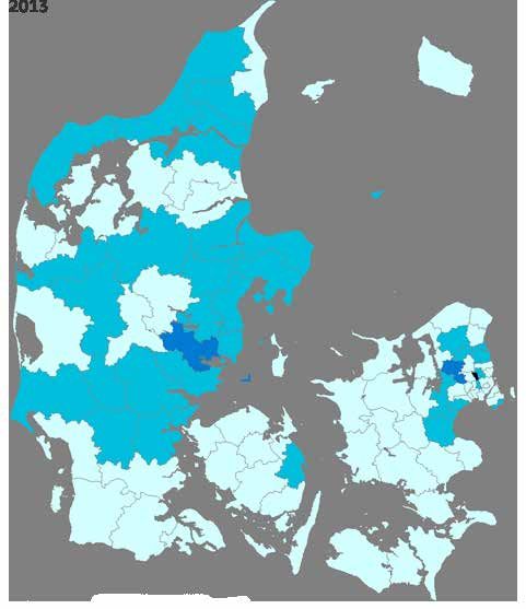
Simulations in the article show that changes in                             ner-occupied flats were about 20 per cent lower
capital gains taxation through a reduction of the                              than their peaks, but in line with prices in early
tax value of interest-rate deductibility would have                            2005, cf. Chart 1 (right).
a relatively modest effect on house prices, espe-                                 The reason why prices of owner-occupied flats
cially in the current very low interest-rate environ-                          rise faster than house prices is that most ow-
ment, as such changes would have only a modest                                 ner-occupied flats are located in large towns and
effect on household interest payments after tax.                               cities, which are seeing the strongest growth. In
A lower value of interest-rate deductibility could                             individual parts of Denmark, price increases of
lead to improved household capitalisation for the                              houses and owner-occupied flats are somewhat
benefit of financial stability.                                                more homogeneous than at the national level.
                                                                                  Owner-occupied flats account for only about
                                                                               11.5 per cent of all owner-occupied homes for
DEVELOPMENTS IN THE DANISH                                                     year-round occupation, cf. Table 1, and are of
HOUSING MARKET                                                                 limited significance to the overall Danish housing
                                                                               market. Below, the primary focus is therefore
Danish house prices have been on the rise since                                on houses. However, in some parts of Denmark,
the spring of 2012, cf. Chart 1 (left). In June 2014,                          owner-occupied flats are quite significant. Just
nominal prices of houses and owner-occupied                                    under 45 per cent of all owner-occupied homes in
flats were up by 1.6 and 10.4 per cent year-on-                                Copenhagen and environs1 are owner-occupied
year. These increases follow a sharp price corre-                              flats, accounting for close to two-thirds of the
ction after the housing bubble of the mid-2000s,                               total value of owner-occupied flats in Denmark in
with prices peaking in 2006-07. In June 2014,                                  2011.
nominal prices of houses and owner-occupied                                       In Denmark, about half of all owner-occupied
floats were 14 and 8 per cent, respectively, below                             homes for year-round occupation are houses
their peak levels. In real terms, house prices were                            owned by private individuals. But developments
approximately 25 per cent lower and prices of ow-                              in this market also depend on other types of

     House prices in Denmark                                                                                                                   Chart 1

                                  Nominal                                                                        Real
     Index, 2000 = 100                                                             Index, 2000 = 100
     225                                                                           225

     200                                                                           200

     175                                                                           175

     150                                                                           150

     125                                                                           125

     100                                                                           100

      75                                                                            75
             00 01 02 03 04 05 06 07 08 09 10 11 12 13 14                                00 01 02 03 04 05 06 07 08 09 10 11 12 13 14
                   Houses           Owner-occupied flats                                       Houses           Owner-occupied flats

     Note:   The 2nd quarter of 2014 is a simple average of monthly observations. In the right-hand chart, nominal prices are deflated by the defla-
             tor for private consumption.
     Source: Statistics Denmark and own seasonal adjustment.

                                                                               1    Copenhagen City comprises the Cities of Copenhagen and Frederiks-
                                                                                    berg and the municipalities of Tårnby and Dragør, while Copenhagen
                                                                                    environs comprise the municipalities of Albertslund, Ballerup, Brønd-
                                                                                    by, Gentofte, Gladsaxe, Glostrup, Herlev, Hvidovre, Høje-Taastrup,
                                                                                    Ishøj, Lyngby-Taarbæk, Rødovre and Vallensbæk.

44                                                                            DANMARKS NATIONALBANK MONETARY REVIEW, 3RD QUARTER, 2014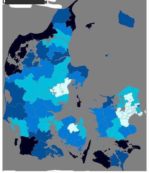
Number of homes for year-round occupation and value of owner-occupied homes,                                                                 Table 1
  broken down by areas

                                                                                                                        Share of value for all of
                                                               Number in thousands
                                                                                                                          Denmark, per cent

                                         Homes
                                      owned by           Owner-                                                                              Owner-
                                         private        occupied Cooperative           Rental flats,      Homes,       Single-family        occupied
                                     individuals            flats   housing                     etc.       other             homes              flats

  Copenhagen City                              33               63             115              137               3               5.3             49.7

  Copenhagen environs                          84               26               16              93             21               13.8             13.5

  Northern Zealand                            112               14                7              39             18               14.8              8.1

  Bornholm                                     16                0                1                2              2               0.6              0.0

  Eastern Zealand                              60                5                6              23             10                6.2              2.5

  Western and southern
  Zealand                                     177                8               12              60             26                9.9              2.8

  Funen                                       138                7                8              57             28                8.2              2.3

  Southern Jutland                            200                9               12              88             37               10.3              3.4

  Eastern Jutland                             202               25               17             117             32               16.0             11.6

  Western Jutland                             132                5                5              44             17                6.7              2.0

  Northern Jutland                            174               11               10              68             26                8.2              4.0

  Entire country                            1,327             173              209              729            220             100.0            100.0

  Note:   The number is calculated as at 1 January 2014. Homes include detached single-family homes, farmhouses, terraced homes, linked
          homes and semi-detached homes, and owner-occupied flats include owner-occupied flats in multi-storey buildings owned by private
          individuals. In the article, owner-occupied flats and homes owned by private individuals are referred to as owner-occupied homes. The
          category of ”Rental flats, etc.” includes rental flats given as multi-storey housing less owner-occupied flats, and student homes in halls of
          residence and residential institutions not owned by a private cooperative housing association. ”Homes, other” include homes owned by
          others than private individuals and private cooperative housing associations. Homes classified under the ownership category of ”Other
          or undisclosed” are homes, multi-storey housing, halls of residence and residential institutions, a total of 80,123, which are not included
          in the table. Values have been calculated based on the Danish Customs and Tax Administration’s property valuation from 2011 and
          comply with the Administration’s property definitions. The total value for the entire country is kr. 2,559 billion for single-family homes
          and kr. 273 billion for owner-occupied flats.
  Source: Statistics Denmark and Danish Customs and Tax Administration.

housing and ownership, since they are, to some                                segments of the housing market with free price
extent, substitutes. Especially in towns and cities,                          formation, including the market for owner-occu-
rental and cooperative housing makes up a high                                pied housing. Hence, rent regulation presumably
percentage of the total housing stock. If housing                             contributes to reinforcing cyclical fluctuations in
demand increases, rental and cooperative hou-                                 the prices of owner-occupied homes, cf. Ministry
sing will be able to absorb some of the demand                                of Economic and Business Affairs et al. (2003)
and the price impact on owner-occupied homes                                     Only a limited segment of the rental housing
will be smaller. However, vacant housing must be                              market is subject to free price formation. Thus,
available for this to occur. Social housing is publi-                         seven out of eight privately rented homes in 2011
cly subsidised, entailing that practically all ten-                           were subject to rent regulation, cf. Danish Tenants
ants of social housing pay a lower rent than they                             Association (2011). Rents in the social housing
would pay for a similar owner-occupied home.                                  sector are not determined by supply and demand
The same applies to most rental housing subject                               either. Moreover, cooperative housing is subject to
to rent regulation. Thus, this housing will not be                            maximum prices, capping the price at which they
vacant, and increased demand must be met by                                   can be sold. If the maximum prices are binding,

DANMARKS NATIONALBANK MONETARY REVIEW, 3RD QUARTER, 2014                                                                                                  45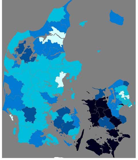
House prices and house sales for selected areas                                                                                   Chart 2

                               House prices                                                                 House sales
     Index, 2000 = 100                                                           Index, 2000 = 100
     225                                                                         170

     200

     175                                                                         120

     150

     125                                                                          70

     100

      75                                                                          20
            00 01 02 03 04 05 06 07 08 09 10 11 12 13 14                               00 01 02 03 04 05 06 07 08 09 10 11 12 13 14
             Denmark                   Copenhagen environs                              Denmark                           Copenhagen environs
             W and S Zealand           Nothern Jutland                                  W and S Zealand                   Nothern Jutland

     Note:   Seasonally adjusted series. Right-hand chart: number of registered sales on the free market.
     Source: Statistics Denmark and own seasonal adjustment.

this is another segment of the housing market that                            sale, totalling about 300 days since early 2012.
is not subject to free price formation. These factors                         That is a long time, emphasising that most of the
seem to indicate a potential for more stable prices                           housing market is struggling. Regional differences
in the market for owner-occupied housing if the                               are also reflected here, since the time on the mar-
overall housing market were deregulated.                                      ket was 345 days in western and southern Zealand
   The housing market is exhibiting different pat-                            in July 2014, or more than twice as long as the
terns across the country. House prices are surging                            time on the market in Copenhagen environs, cf.
in large towns and cities, particularly Copenha-                              Chart 3 (left).
gen, while they are falling in other parts of the                                There is a marked tendency for the largest
country, cf. Chart 2 (left). In Copenhagen City, the                          price reductions to be given in areas with weak
annual rate of price increase in the 1st quarter                              housing markets, cf. Chart 3 (right). Large price
of 2014 was 12 per cent for owner-occupied flats                              reductions indicate that the seller and buyer ge-
and 9.3 per cent for houses, while house prices                               nerally do not agree on the price. This also makes
in western and southern Zealand declined by 0.7                               the sale less feasible.
pct. In northern Jutland, house prices have remai-                               The seasonally adjusted number of enforced
ned largely unchanged since early 2009, albeit                                sales has stabilised at around 300 per month,
with a slightly decreasing trend.                                             albeit with some variation from one month to the
   The differences in the housing market are also                             next. The number of enforced sales has declined
reflected in trading activity, cf. Chart 2 (right). Sin-                      over the last two and a half years from just over
ce 2011, annual house sales have been totalling                               450 per month. During the same period, mortga-
approximately 32,500 houses, equivalent to just                               ge arrears have fallen, dropping to approximately
two-thirds of the average since 1995. However, in                             0.25 per cent in the last few quarters. The arrears
Copenhagen environs house sales are up, in 2013                               rate indicates the proportion of total payments
almost reaching the average since 1995. In we-                                that had not been made 105 days after the due
stern and southern Zealand, sales in 2013 remai-                              date. The decline in the number of enforced sales
ned roughly unchanged from the previous couple                                has been distributed evenly across regions, alt-
of years, the level slightly over half of average                             hough there are still considerable regional diffe-
sales since 1995.                                                             rences, cf. Chart 4. Municipalities in western and
   During the last few years, the supply of houses                            southern Zealand have a particularly high number
on the market has amounted to just over 40,000.                               of enforced sales relative to the number of ow-
High supply and low turnover have an impact on                                ner-occupied homes.
the average time on the market for a house for                                   In summary, house prices are increasing at the

46                                                                            DANMARKS NATIONALBANK MONETARY REVIEW, 3RD QUARTER, 2014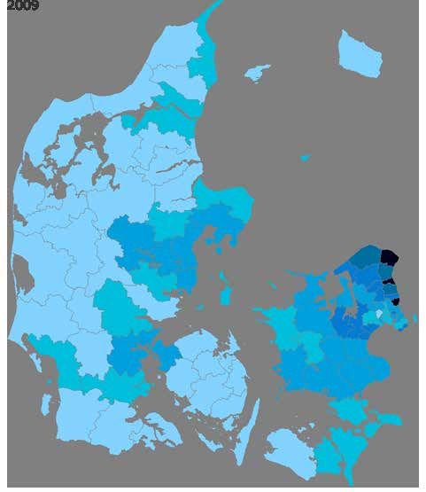
Time on the market and price reductions on house sales, selected areas                                                                    Chart 3

                         Time on the market                                                            Price reductions
  Number of days                                                              Per cent
  450                                                                         25

   375
                                                                              20
   300
                                                                              15
   225
                                                                              10
   150

    75                                                                          5

     0                                                                          0
          04 05 06 07           08    09    10 11 12 13 14                           04 05 06 07 08              09    10 11 12 13 14
          Denmark                            Copenhagen environs                      Denmark                            Copenhagen environs
          W and S Zealand                    Nothern Jutland                          W and S Zealand                    Nothern Jutland

  Note:   Seasonally adjusted series. Right-hand chart: price reductions are given as the spread between the initial asking price and the sales
          price relative to the initial asking price.
  Source: Housing Market Statistics.

                                                                             However, this masks substantial regional differen-
  Enforced sales as a percentage of the                      Chart 4
                                                                             ces; prices, turnover and supply, etc. are showing
  stock of owner-occupied housing
                                                                             different patterns with considerable variation in
                                                                             levels.
                                                                                The diverging trends also reflect the self-re-
                                                                             inforcing mechanisms in the housing market.
                                                                             Increasing prices could encourage households to
                                                                             buy a home, expecting that its price will continue
                                                                             to rise, so that they will make a capital gain from
                                                                             homeownership. This will boost demand for hou-
                                                                             sing and could cause prices to escalate further.
                                                                             Conversely, households could be hesitant to buy
                                                                             a home if prices are falling or they expect them to
                                                                             fall. The delay in demand could reinforce a dow-
                                                                             nward trend in house prices.
                                                                                Moreover, since homes sold through enforced
                                                                             sale tend to be sold at a substantial discount to
                                                                             the market value, a large number of enforced
                                                                             sales in a given area could have a negative effect
                                                                             on house prices. This also reduces the probability
                                                                             of selling a home on the market. If the owner is
     0.00-0.09         0.10-0.19        0.20-0.29
                                                                             having trouble meeting his mortgage payments,
     0.30-0.39         0.40-1.00
                                                                             longer time on the market increases the risk of en-
                                                                             forced sale. Moreover, in itself, low turnover adds
  Note:   Number of enforced sales from July 2013 to June 2014.
          Enforced sales and housing stock are calculated for all            to the risk that a home cannot be sold on the
          owner-occupied homes, including leisure homes.                     market and has to be sold through enforced sale.
  Source: Association of Danish Mortgage Banks.
                                                                             At the same time, uncertainty as to the proper
                                                                             price of a home increases with few recent sales for
                                                                             comparison.
national level, but the housing market as a whole                               To identify the causes of the regional differen-
is still struggling with low turnover, a substantial                         ces, the factors determining housing supply and
housing supply and a long time on the market.                                demand are examined below.

DANMARKS NATIONALBANK MONETARY REVIEW, 3RD QUARTER, 2014                                                                                              47
HOUSING DEMAND                                                            in a large disposable amount for other expenses.
                                                                          Part of the disposable amount is probably saved
House prices, like prices of any other commodi-                           to allow homeowners to pay future interest costs
ty, are determined by supply and demand. But,                             when interest rates are likely to be higher. Thus,
unlike most other markets, prices in the housing                          the current low interest rates are hardly fully re-
market do not adjust instantaneously to match                             flected in housing demand and house prices. This
supply to demand. This is due to the housing mar-                         relationship is in line with the high current level of
ket’s special characteristics – for example indivi-                       household savings.
dual homes vary substantially, much time is spent
searching for a home and the costs of changing                            DEMOGRAPHICS
homes are high.                                                           Housing demand is also determined by demo-
    Demand for housing is usually assumed to be                           graphics. Population growth fuels demand, and
determined by household disposable income                                 the age composition has a bearing on the types
and the user cost, i.e. the cost of owning a home.                        of homes in demand. At present, Denmark is
The user cost includes real interest rates after tax,                     experiencing population growth in the order of
housing-related taxes, depreciation and mainten-                          30,000 people a year due mainly to net immigrati-
ance and the expected real capital gain or loss in                        on, which increases total housing demand.
the form of changed house prices, which ex ante                              Recent years have seen substantial migrati-
are subject to great uncertainty.                                         on from rural to urban areas. For instance, the
    Moreover, first-year payments may be signifi-                         combined population of the Cities of Copenhagen
cant to households. The reasons are that, in addi-                        and Frederiksberg has grown by a total of 60,000
tion to the financial user cost, some families also                       inhabitants since early 2009, equivalent to 10 per
attach importance to their liquidity position, have                       cent, while the number of inhabitants in the mu-
limited access to loans or find it easier to relate to
the payment to be made now than to the calcula-
tion underlying a residential investment over its
entire lifetime, cf. the discussion in Dam et al.                            Percentage change in the number                       Chart 5
                                                                             of inhabitants from 1 January 2009 to
(2011a). Badarinza et al. (2014) analyse the choice                          1 July 2014
between short-term and long-term interest rates
on household mortgage loans across nine coun-
tries (including Denmark), finding that, in their
choice of financing, households tend to focus on
short-term costs and liquidity.
    Based on the Danish figures, it cannot be de-
termined whether the first-year payments have a
separate impact on Danish house prices. Statisti-
cally, the relation obtained by including the lowest
possible first-year payments is neither better nor
worse than a relation based solely on the pure user
cost.2 However, the economic arguments mentio-
ned are deemed to be strong enough for first-year
payments to be included in the demand relation
for housing used in this article, cf. the Appendix,
which describes the model used in the article.
    The current extraordinarily low interest rates
mean very low borrowing costs, especially for
homeowners with loans based on short-term in-                                   [-9.3]-[-4.1]    [-4.0]-[-2.1]   [-2.0]-[-0.1]   0.0-1.9
terest rates. Other things being equal, this results                            2.0-3.9          4.0-5.9         6.0-13.0

2    This requires that inflation expectations are down-weighted in the      Source: Statistics Denmark.
     real interest rate expression.

48                                                                        DANMARKS NATIONALBANK MONETARY REVIEW, 3RD QUARTER, 2014
nicipality of Lolland has been reduced by 4,400,                           Consequently, the future demand for urban hou-
corresponding to a decline of more than 9 per                              sing will increase, while the demand for housing
cent, cf. Chart 5.                                                         in peripheral areas will decrease. This is especial-
   According to Statistics Denmark’s most recent                           ly true when demographic factors such as age,
population projection, urban population growth                             education and cohabitation patterns are taken
is set to continue at the expense of rural areas.                          into account, cf. Hansen et al. (2013).

  Interaction between regional housing markets                                                                                             Box 1

  A ripple effect exists between regional housing markets,                 pulation of Copenhagen remained largely unchanged, while
  cf. Meen (1999 and 2001). This effect is created through                 it increased in the surrounding areas. When prices subse-
  multiple channels, the most import channel seeming to be                 quently fell in Copenhagen, narrowing the price difference,
  the price. A growing price spread between two areas implies              the population of Copenhagen started growing rapidly.
  that more of the demand will be aimed at the area with the               In recent years, prices have been escalating in Copenha-
  lowest price, contributing to some geographical equalisati-              gen, thereby increasing price differences, and at the same
  on – both in terms of price and activity. But price differences          time, the population of Copenhagen continues to grow, for
  should be seen in the context of distances. The closer two               instance because people are not moving out to the same
  areas are, the closer substitutes the general location of                extent as seen in the first half of the 2000s.
  housing will be. Accordingly, in general, Danish house prices                 However, in 2012 and 2013, slighly more people in the
  are lower, the further the distance to the nearest urban area            25-39-year age group moved out of Copenhagen than in the
  with high prices, cf. the chart below (left). Heebøll (2014)             preceding years, most of them moving to municipalities in
  finds indications that price developments in Copenhagen                  eastern and northern Zealand. At the same time, higher pri-
  seem to lead prices in the rest of the country.                          ces in Copenhagen once again seem to be rippling through
      In the mid-2000s, surging prices in Copenhagen caused                to eastern Zealand, but this time the effect starts at a higher
  the price difference between Copenhagen and other areas                  price difference per square metre of home than in the 2000s,
  of Zealand to increase, having a ripple effect from Copenha-             cf. the chart below (right).
  gen to the surrounding areas. During that period, the po-

  Average price in kr. 1,000 per square metre of home 2013/14 (left) and additional price per square me-
  tre of home in Copenhagen environs relative to the closest surrounding areas (right)

                                                                             1,000 kr.                                                1,000 kr.
                                                                             18                                                              28
                                                                             16                                                              26
                                                                             14                                                              24
                                                                             12                                                              22
                                                                             10                                                              20
                                                                              8                                                              18
                                                                              6                                                              16
                                                                              4                                                              14
                                                                              2                                                              12
                                                                              0                                                              10
                                                                                  00 01 02 03 04 05 06 07 08 09 10 11 12 13

                                                                                          Northern Zealand
                                                                                          Eastern Zealand
                                                                                          Western and Sourthern Zealand
                                                                                          Level for Copenhagen environs (right axis)

     0.0-5.9          6.0-7.9           8.0-9.9
     10.0-14.9        15.0-19.9         20.0-34.9

  Note:   Left-hand chart: average sales price in the period from the 2nd quarter of 2013 to the 1st quarter of 2014. Prices have not been adju-
          sted for potential quality differences between the homes sold. Right-hand chart: Seasonally adjusted data. 3-quarter moving averages.
  Source: Housing Market Statistics.

DANMARKS NATIONALBANK MONETARY REVIEW, 3RD QUARTER, 2014                                                                                           49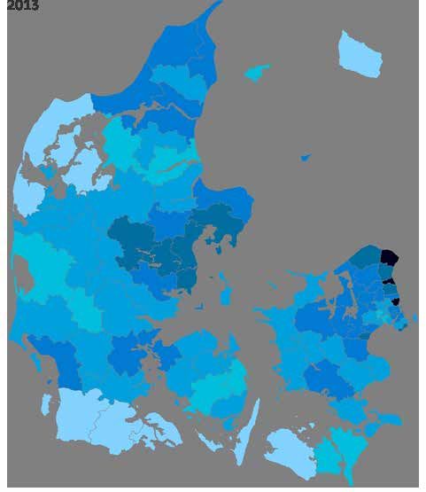
Interaction between regional housing markets                                                                                     Box 1 continued

     The reason why higher prices in Copenhagen are rippling                    ced using a fixed rate loan with amortisation, the differences
     through later this time could be that – due to the decline                 in the 1st quarter of 2014 were in line with those in 2006, at
     in interest rates – the difference between financing costs                 at their peak, cf. the chart below (right).
     and housing taxes in Copenhagen and environs relative                          Expectations in terms of the future user cost could also
     to other Danish areas has not increased similarly. This is                 help explain growing price differences. This is the case if
     particularly true for homes financed with variable rate and                people base their expectations of price patterns on histori-
     deferred amortisation loans. With this type of financing, the              cal performance. If prices have been appreciating for some
     difference between financing costs and tax payments on a                   time, as seen in Copenhagen, people may expect to make a
     home in Copenhagen environs and other Zealand areas was                    capital gain from homeownership. This will reduce the expe-
     generally smaller in the 1st quarter of 2014 than during the               cted user cost and boost housing demand. Conversely, fal-
     period from the 2nd half of 2005 to 2008, cf. the chart below              ling prices, as seen in western and southern Zealand, could
     (left), although the difference in price per square metre was              cause them to anticipate a capital loss. This will increase the
     smaller at the time. If, instead, the home purchase is finan-              user cost and reduce housing demand.

     Savings in annual financing costs and tax payments related to homeownership in selected areas rather
     than in Copenhagen environs

     Kr. 1,000 Variable-rate loan without amortisation Kr. 1,000                  Kr. 1,000      Fixed-rate loan with amortisation         Kr. 1,000
     100                                                     180                  150                                                            250

      80                                                             160
                                                                                  100                                                             200
      60                                                             140

      40                                                             120
                                                                                   50                                                             150
      20                                                             100

        0                                                            80              0                                                            100
             04 05 06 07 08 09 10 11 12 13 14                                            02 03 04 05 06 07 08 09 10 11 12 13 14
                 Northern Zealand                                                             Northern Zealand
                 Eastern Zealand                                                              Eastern Zealand
                 Western and Southern Zealand                                                 Western and Southern Zealand
                 Level for Cph's environs (right-hand axis)                                   Level for Cph's environs (right-hand axis)

     Note:   The series illustrate stylised financing costs, including administration margins, brokerage fees and housing taxes on the purchase of a
             single-family home of 140 square metres.
     Source: Statistics Denmark, Housing Market Statistics, Realkredit Danmark, Danmarks Nationalbank and own calculations.

   However, demographic developments should                                     tenants. More students thus increase the pressure
be seen also in the context of prices. Urban popu-                              on the rental housing market; however, to address
lation growth could be the result of the narrowing                              the issue of rental housing shortages, parents are
difference in the sum of financing payments and                                 buying flats for their student and adult children,
tax payments between Copenhagen and the sur-                                    boosting demand for owner-occupied housing.
rounding areas since the mid-2000s, cf. Box 1.                                     The population growth in Copenhagen has
   People under the age of 30 account for ap-                                   been broad-based across age groups below 60,
proximately 60 per cent of the population grow-                                 while the number of people in their early 60s or
th in the City of Copenhagen, reflecting mainly                                 older than 75 has declined. However, the fall is
that more young people have migrated to towns                                   limited and has released relatively few homes.
and cities, often to study, and that an increasing
proportion of people have remained in or around                                 DISPOSABLE INCOME
Copenhagen after graduation. They have subse-                                   The changes in demographic patterns should be
quently started families, so the number of children                             seen in the context of uneven distribution of eco-
in Copenhagen has increased. Families with chil-                                nomic growth across Denmark since 2008. Growth
dren tend to demand larger homes – in Copenha-                                  has primarily taken place in the cities, especially
gen often in the form of owner-occupied homes.                                  Copenhagen, which has also seen the largest
Students typically have low incomes and are                                     rise in employment. As a result, the labour force

50                                                                             DANMARKS NATIONALBANK MONETARY REVIEW, 3RD QUARTER, 2014
plies to other large towns and cities in Denmark.
House price of an average home rela- Chart 6
Accordingly, people who can afford owner-occu-
tive to average disposable household
income pied housing are increasingly living in the cities,
serving to increase demand. Since Copenhagen’s
Index, 2000 = 100 housing supply has not grown in line with de-
160
mand, this is reflected in higher prices.
140 The level of house prices may be seen in
relation to household disposable income, since
120
the disposable income usually finances the home
100 purchase. In the last few years, the price of an
average home has increased at the same rate as
80
the average household disposable income and
60 the ratio between the two is largely the same as
in 2004, i.e. before the surge in house prices, cf.
40
92 94 96 98 00 02 04 06 08 10 12 14 Chart 6.
Note: Household disposable income excluding pension savings INTEREST RATES AND TAXES
divided by the number of households in Denmark, i.e. The price of an average home relative to average
both owners and tenants. An average home is 140 squa-
re metres. household disposable income is a simplified way
Source: Statistics Denmark and Housing Market Statistics.
of looking at the level of house prices. The reason
is that changes in interest rates and taxes, among
other factors, are not taken into account although
in Copenhagen has expanded in recent years, they are very important in terms of current costs
while it has decreased in the rest of the country, of financing homeownership.
reflecting, inter alia, that jobholders are moving In recent years, interest rates, both short-term
to urban areas, while the unemployed and pensio- and long-term, have declined to very low levels,
ners are increasingly moving to other parts of the cf. Chart 7 (left). Low interest rates make mortga-
country. At the same time, average incomes have ge financing less expensive, helping to buoy up
risen more in Copenhagen than in the rest of the the housing market. However, a small part of the
country, due, among other factors, to an increase interest rate fall has been offset by higher admi-
in the average level of education. The same ap- nistration margins and brokerage fees, especially
Interest rate developments and housing burden Chart 7
Interest rate developments Housing burden
Per cent Per cent
8 40
35
6
30
4 25
20
2
15
0 10
00 01 02 03 04 05 06 07 08 09 10 11 12 13 14 81 84 87 90 93 96 99 02 05 08 11 14
Fixed rate, w/amortisation
30-year mortgage yield Fixed rate, w/o amortisation
Short-term mortgage yield Variable rate, w/amortisation
Variable rate, w/o amortisation
Note: The housing burden for the 2nd quarter of 2014 is based on expected developments in house prices and household disposable income
in the projection described in this Monetary Review. The housing burden illustrates stylised financing costs including administration
margins, brokerage fees and housing taxes on the purchase of a single-family home of 140 square metres as a percentage of the avera-
ge income. See Dam et al. (2011a) for further details.
Source: Statistics Denmark, Housing Market Statistics, Realkredit Danmark, Danmarks Nationalbank and own calculations.
DANMARKS NATIONALBANK MONETARY REVIEW, 3RD QUARTER, 2014 51for the most risky loans, i.e. variable rate or defer- housing stock if supply is to be reduced. Thus,
red amortisation loans. supply is fixed in the short term, and the price is
Measured in terms of Danish kroner, housing determined by demand.
taxes are relatively stable over time due, inter alia, The value of a home is comprised of the physi-
to the nominal freeze on property value tax intro- cal value of the home and its location. The phy-
duced in 2002; however, property value tax will sical value is presumably given by construction
be reduced correspondingly if the property value costs, at least in the medium term, since, with a
falls below the 2002 level. Moreover, there is a cap certain lag, housing units may be constructed in
on year-on-year increases in property tax – known the required number. Initiating new construction
as land tax – in the form of a regulation ratio. As projects will be financially attractive if the physical
a result of these rules, the effective tax rate is not value of existing housing exceeds the cost of new
the same across Denmark. In areas with rising construction. This process will continue until the
house prices since 2002, tax payments have not supply has been increased enough for the price
increased correspondingly and thus account for a of housing to have fallen to the level of construc-
lower percentage of the value of the home. Con- tion costs. If this anchoring of house prices is
versely, areas where house prices have remained generally known and understood by the market,
largely flat since 2002 have not benefited from the speculative element will be dampened, and
a lower effective tax rate. In practice, this entails unsustainable, speculation-fuelled price hikes will
that the effective tax rate on housing is lower in be limited.
Copenhagen than in large parts of the Danish Conversely, if the increase in housing demand
provinces, for example western and southern Zea- turns out to be transient in nature (a so-called
land. Copenhagen’s lower tax rate boosts demand temporary demand shock), the housing supply
and raises house prices, generating capital gains adjustment will cause the subsequent price drop
for current homeowners. to be stronger than it would otherwise have been.
Overall, current costs of financing homeow- This is because there is more housing on the
nership relative to average household disposable market than previously, potentially in the form
income have dropped sharply at the national level of upcoming housing projects, since much of the
in recent years. This is demonstrated by the devel- residential construction may have been planned
opment in the housing burden, cf. Chart 7 (right). and initiated before the reversal and would not be
Obviously, financing costs vary with the type of financially viable to cancel.
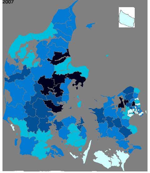
loan, but – regardless of the type of loan – the That seems to have been the case in some
housing burden is lower today than in the early places in Denmark, which experienced a residen-
2000s before house prices started soaring. This is tial construction boom in 2007, cf. Chart 8 (left),
due to the very low interest rates. although demand was already weakening and
If the home purchase is financed through a prices were falling faster than justified by the hig-
fixed-rate loan with amortisation, the housing her supply. Subsequently, residential construction
burden in the 2nd quarter of 2014 was 27 per has been very limited, indicating an oversupply of
cent, or just over 2 percentage points lower than housing. Accordingly, no further construction has
the average since 1981. For other loan types, the been required, cf. Chart 8 (right), among other
housing burden was considerably lower. things because demand is or has been falling as
a result of migration. Oversupply of housing has a
number of negative effects on the housing mar-
DEMAND AND LAND PRICES ket, cf. Box 2.
Unlike the actual housing unit, the location can-
The housing market differs from many other not be produced in unlimited numbers. Geograp-
markets in that supply responds to changes in hy largely determines whether land shortages
demand with a considerable lag. Planning and exist. In rural areas, land is in ample supply, while
completing new construction projects takes time large towns and cities have a shortage of land.
if supply is to be increased; similarly, the housing This is reflected in substantial differences in land
decay rate is slow, entailing that it takes a very prices across Denmark, cf. Chart 9 (left). In rural
long time for housing to be eliminated from the areas, the price reflects alternative land uses, typi-
52 DANMARKS NATIONALBANK MONETARY REVIEW, 3RD QUARTER, 2014Completed construction for year-round occupation as a percentage of the existing Chart 8
housing stock in 2007 and 2013
0.0-0.6 0.7-1.1 1.2-1.7 0.0-0.6 0.7-1.1 1.2-1.7
1.8-2.1 2.2-3.3 1.8-2.1 2.2-3.3
Note: Completed construction in square metres as a percentage of the total floorage. Both for year-round occupation.
Source: Statistics Denmark.
Land prices in selected areas and development in house prices, construction costs, land Chart 9
prices and consumer prices
Land prices House and land prices, etc.
Kr. 1,000 Index, 2000 = 100 Index, 1955 = 1
3,000 150 90
Hundreder
2,500 125 75
2,000 100 60
1,500 75 45
1,000 50 30
500 25 15
0 0 0
92 94 96 98 00 02 04 06 08 10 12 55 59 63 67 71 75 79 83 87 91 95 99 03 07 11
Copenhagen environs Northern Zealand
Eastern Zealand W and S Zealand House prices Construction costs
Northern Jutland Denmark (right axis) Land prices Consumer prices
Note: Left-hand chart: simple average of prices of sold plots below 2,000 square metres for the area. For the series ”Denmark”, a price index
is shown in which Statistics Denmark has quality-adjusted data based, inter alia, on the public property valuation. Right-hand chart: all
indices illustrate developments in nominal prices and costs.
Source: Statistics Denmark.
DANMARKS NATIONALBANK MONETARY REVIEW, 3RD QUARTER, 2014 53The housing market in case of an oversupply of housing Box 2
There are considerable geographical differences in the ban migration trends will reverse anytime soon, permanent
number of homes for sale and the number of unoccupied changes in the housing supply are required if the balance
homes, cf. the chart below (left). Some are unoccupied for a between supply and demand is to be restored. As homes
short period of time while people are moving house, so the are slow to lose their value and will continue to be part of
percentage of unoccupied homes will never be zero. More- the supply for a long time even if they are not maintained,
over, some homes are unoccupied because they are used as this process will take many years. When the oversupply is
leisure homes, while the rest is de facto unoccupied. eventually absorbed, the price will, once again, be given by
In some parts of Denmark, the high percentage of ho- construction costs plus land prices.
mes for sale and unoccupied homes indicates that supply In practice, the supply will decline when homes are
exceeds demand, which will lead to lower prices. Experien- demolished or fall into such disrepair as to be uninhabi-
ce shows that some stickiness exists in this respect, since table. If a home is uninhabitable, it typically has not been
homeowners are not immediately prepared to accept a loss maintained for many years. This may be the case if house
on their home or have debt exceeding the price that would prices are low, since this provides a disincentive to maintain
ensure a sale. Consequently, the initial asking price tends to the home because the costs incurred will not be covered
be higher than the final sales price, especially if the home by a potential sale. Demolition is costly, and conversion to,
is on the market for some time in a declining price environ- say, agriculture may not be profitable. Financially, the best
ment. Moreover, people will be hesitant to buy if they expect option may be to let the home fall into disrepair and pay the
prices to fall, since they expect to be able to acquire a home taxes due. Thus, demolition subsidies, as agreed in the June
later at a lower price. This will be reflected in low turnover 2014 growth package, may help to speed up the housing
and a long time on the market in areas with an oversupply adjustment process in selected parts of the country. Alterna-
of housing. tively, demand in these areas may be boosted by improving
In most of the areas with a large supply of housing, tax deductions for commuters or by increasingly dispensing
declining demand is due to demographic changes, including from the principal residency requirement to allow homes for
rural-to-urban migration. As there are no indications that ur- year-round occupation to be used as leisure homes.
Unoccupied homes and homes for sale as a percentage of the total number of homes for
year-round occupation
2.0-3.9 4.0-5.9 6.0-7.9 1.5-1.9 2.0-2.4 2.5-2.7
8.0-9.9 10.0-32.2 2.8-2.9 3.0-3.4
Note: Left-hand chart: number of homes with no registered inhabitants as at 1 January 2014 relative to the total number of homes for year-
round occupation in the municipality. Some of the homes with no registered inhabitants are used as leisure homes. As they cannot be
identified by Statistics Denmark, they are not included in the statistics. Right-hand chart: seasonally adjusted number of homes for sale
in July 2014 relative to the number of farmhouses, detached single-family homes, terraced homes, linked homes and semi-detached
homes as well as owner-occupied flats in the area as at 1 January 2014.
Source: Statistics Denmark and Housing Market Statistics.
54 DANMARKS NATIONALBANK MONETARY REVIEW, 3RD QUARTER, 2014cally forestry and agriculture, as well as the cost of that urbanisation trends are being reversed. Hig-
land development. In urban areas, the supply can, her urban population density will produce increa-
at some point, no longer be increased. Alternati- ses in urban land values, and if the residential
vely, it will be difficult and costly to increase the area expands, this will drive up land values on the
area of building land, for instance if polluted areas outskirts of towns and cities as the alternative use
are to be cleaned up or new building land is to be changes from agriculture to residential.
created by building out into the water. Thus, land
prices will increase until demand matches supply. LAND PRICES IN A HOUSE PRICE MODEL
The scarcer the land, the more land prices need There has been a clear, long-term tendency for
to fluctuate in order for changes in demand to land prices to rise, cf. Chart 9 (right), reflecting
be adjusted to the largely fixed supply. While, to that economic growth has increased the demand
some extent, construction costs have a cyclical for land, for example for residential purposes, but
element, not least due to wage developments in also for other purposes such as agriculture.
the construction sector, land prices tend to fluctu- Hence, including land prices in a house price
ate more widely, cf. Chart 9 (right). Since land pri- model is relevant. In the model used in this article,
ces account for a much higher proportion of total it has been assumed that house prices are compo-
house prices in large towns and cities, urban price sed of two components: the price of the house it-
fluctuations will be stronger than those experien- self and the land price. The weight to be attached
ced in rural areas. to each component depends on the shortage of
The price of a building plot depends not just land available, which varies across the country.
on the discounted value of future returns, e.g. in In the model, residential construction re-
the form of housing occupancy if the plot is used sponds when the actual house price deviates
for housing construction, but also on the fact from construction costs, while land prices have
that the land could become more valuable in the no significance. In the absence of sufficiently valid
future, cf. Titman (1985). If the price of the plot is and reliable land price data, cf. Box 3, land pri-
expected to appreciate, the owner will sell it only ces are assumed to grow in line with household
at a price that is high enough to compensate him disposable income. Thus, indirectly, it is assumed
for not obtaining the expected higher price at a
later time. This may explain why the supply and
turnover of new building plots are highly limited
during periods of low or falling prices. This helps Statistics for building plot prices Boks 3
to stabilise house prices by limiting the supply of Statistics Denmark calculates a price index and the price
new housing in a weak market. per square metre and the average price of plots below
2,000 square metres. These statistics provide an indica-
However, if growth in the housing market fuels
tion of building-plot prices, although this category does
expectations that prices will continue to rise for not distinguish between the purposes of the plot, i.e. if it
some time – e.g. during a housing bubble – the is intended for housing, leisure or business purposes.
estimated option value of land could contribu- The prices in the statistics sometimes fluctuate
sharply, especially during certain periods and in certain
te to sustaining the upswing. This occurs when
areas, cf. Chart 9 (left), as the statistics are sometimes
landowners withhold plots from sale in the expe- based on very few observations – for instance because
ctation of being able to sell them later at an even a small number of trades causes random fluctuations.
higher price. This reduces supply during a period Furthermore, in its quality adjustment Statistics Denmark
eliminates many observations.
of high demand, causing the price pressure to in- More fundamentally, a house-price model also
crease. These relationships highlight that land and needs the prices of plots already built up. However, the
houses are investment objects and that expecta- statistics only contain observations of the sales prices
of unbuilt plots. That is hardly significant in rural areas,
tions of future price developments could have a
but in urban areas unbuilt plots are often located on the
considerable impact on current price movements. outskirts of towns and cities, and the location cannot be
The option value of a plot is higher in and compared with built-up plots in the town or city centre.
around towns and cities, reflecting that urban Thus prices are not available for plots located in areas
where land is scarce. These plots fetch the highest prices,
land prices are both higher and more volatile. Mo-
and their prices tend to fluctuate more, since a higher
reover, future housing demand is likely to focus supply cannot dampen price rises.
on towns and cities, since there are no indications
DANMARKS NATIONALBANK MONETARY REVIEW, 3RD QUARTER, 2014 55that the demand for scarce land is growing in line MODEL SIMULATIONS
with household disposable income. The modelled
relationship is to capture the long-term trend for House prices are influenced by a range of factors,
real house prices to rise in response to the increa- including cyclical movements, economic policy
sing shortage of land in large towns and cities, and financial conditions. Politicians decide how
while short-term movements in land prices have and how much housing should be taxed, includ-
not been modelled. ing the tax value of mortgage rate deductibility.
Thus, persistent income shocks have a per- At the same time, monetary policy impacts the
manent effect on house prices; furthermore, the housing market through interest rates. Institutio-
long-term income elasticity of housing demand nal aspects, such as the maximum permitted LTV
is assumed to be one. The latter should be seen ratio or the upper limit for deferred amortisation
in the context that housing consumption cannot mortgages, may also be significant.
exceed income, and that the saturation point will Below, the effects of a number of these fac-
occur somewhat earlier, cf. Dam et al. (2011a). tors are quantified using the house-price model
Moreover, the ratio of housing costs to disposable described above and in the Appendix. The model
income varies across the country. In towns and simulates the effects on house-price movements
cities, land is scarce and prices are high, mea- of changes in interest rates, deferred amortisation
ning that the ratio is higher than in the provinces and interest rate deductibility.
where prices are low. As more people migrate to
towns and cities, the number of people spending INTEREST RATE CHANGES AND INTEREST RATE
a large percentage of their income on housing EXPECTATIONS
costs is set to increase. While this adjustment Interest rates are important in determining hou-
process is ongoing, housing costs will absorb sing demand – and thus house prices. The impact
a higher percentage of household income. The is through the user cost, real interest rates after
increasing budget share of housing costs, at the tax accounting for a key portion of the costs of
aggregate level, in recent decades should be seen homeownership. Furthermore, short-term interest
in this context. When the shift in the settlement rates are included in the first-year payments.
patterns ends, the ratio of housing costs to hou- To illustrate the significance of interest rates
sehold income may stabilise. changes, simulations of the house-price model are
House prices under different interest rate assumptions Chart 10
Mortgage yields House prices, deviation from baseline scenario
Per cent Per cent
5 40
4 30
3 20
2 10
1 0
0 -10
14 16 18 20 22 24 26 28 30 16 19 22 25 28 31 34 37 40 43 46 49
1 year, baseline 30 years, baseline
Scenario 1
1 year, scenario 1 30 years, scenario 1
1 year, scenario 2 30 years, scenario 2 Scenario 2
Note: Left-hand chart: ”1 year” is the interest rate on a variable rate loan with a maturity of 1 year. ”30 years” is the interest rate on a 30-year
fixed rate loan. In the baseline scenario, gradual normalisation of interest rates up until 2020 is assumed. In scenario 1, interest rates are
maintained at a low level for the end of 2016 onwards. Scenario 2 entails slower normalisation of interest rates; full normalisation is not
expected to occur until 2024.
Source: Own calculations.
56 DANMARKS NATIONALBANK MONETARY REVIEW, 3RD QUARTER, 2014used. These simulations are based on Danmarks
Nationalbank’s projection presented in this Mone- Expiry of the period of deferred Chart 11
amortisation
tary Review, expanded by a technical projection
from 2017 onwards. The projection entails, inter Kr. billion
alia, a gradual increase in interest rate levels to 175
long-term levels determined on the basis of inte- 150
rest rates over recent decades. Thus, the rate of 125
interest on 1-year adjustable rate loans is increa-
100
sed to 3.5 per cent, while the 30-year interest rate
75
is increased to 5 per cent, cf. the baseline scenario
50
in Chart 10 (left). In the simulations, the baseline
scenario is compared with two different scenarios. 25
In all the simulations performed, the rate of inflati- 0
14 15 16 17 18 19 20 21 22 23
on is assumed to be just under 2 per cent a year. LTV < 60 60 < LTV < 80 80 < LTV < 100 LTV > 100
In scenario 1, both the 1-year and the 30-year
interest rates are maintained at the low level for Note: LTV is short for loan-to-value, expressing the relationship
2016 from the projection presented in this Mone- between the amount of the loan and the value of the
home.
tary Review. Short-term interest rates are part of Source: Danish mortgage banks, Danmarks Nationalbank and
the first-year payments, while long-term interest own calculations.
rates are included in the user cost. This results in a
substantial price reaction, since the model proje-
cts that in 2024, prices will be 32 per cent higher economy, cf. Andersen et al. (2014). A lower limit
than in the baseline scenario, then slowly fall for deferred amortisation would reduce LTV ratios
back, cf. Chart 10 (right). in boom periods, thereby preventing them from
In scenario 2, it is assumed that actual interest becoming excessive in recession periods.
rates rise more slowly towards their long-term The use of deferred-amortisation mortgage lo-
levels than projected by the baseline scenario. ans for owner-occupied homes and summer cot-
Again, lower interest rates lead to stronger price tages grew strongly from the introduction in 2003
movements: in 2023, prices are 11 per cent higher to the outbreak of the financial crisis, accounting
than in the baseline scenario. Prices fuel residen- for close to 50 per cent of total mortgage lending
tial construction. Higher supply and adaptive at end-2008. Since then this share has increased
household expectations of housing capital gains to more than 55 per cent. Around half the loans
mean that once price increases have peaked, they have an LTV ratio of more than 80 per cent and by
will relatively quickly fall to around zero, before far the largest number of loans has an LTV ratio
gradually stabilising. of more than 60 per cent, cf. Chart 11. This makes
The simulations illustrate that house prices households sensitive to even small declines in
are highly sensitive to interest rate movements. house prices, and mortgage banks may have to
Therefore, widespread expectations that the fund top-up collateral for bonds.
current low interest rates will persist for a number Changing the upper limit for deferred amortisa-
of years entail a substantial risk that house prices tion does not affect the user cost – it only defers
could escalate in the short to medium term. the loan repayment date. But it does have an
immediate impact on liquidity through the first-
DEFERRED AMORTISATION year payments. Calculations show that for a fully
During the most recent boom, household bor- leveraged purchase of an average home using a
rowing surged. When house prices subsequently fixed-rate mortgage, the monthly payment in the
began to fall, LTV ratios increased substantially. 2nd quarter of 2014 would e.g. have been just un-
Analyses show that the high gross debt does der kr. 850 higher with an LTV ratio of 60 per cent
not pose a serious threat to financial stability, cf. rather than 80 per cent.
Andersen (2012). On the other hand, the high As discussed above, there are strong econo-
debt may have indirect effects, since high LTV mic arguments that the first-year payments affect
ratios amplify cyclical fluctuations in the Danish housing demand. But since, based on statistical
DANMARKS NATIONALBANK MONETARY REVIEW, 3RD QUARTER, 2014 57criteria, it cannot be determined whether the first-
Effect on annual rate of price increase Chart 12
year payments indeed have a separate impact on
for house prices if the upper limit for
deferred amortisation mortgage loans is Danish house prices, it cannot be ruled out either
reduced from 80 to 60 per cent that changes in the access to deferred amortisati-
on loans may have only a modest effect on house
Percentagepoints
1.5 prices. Therefore, the reported results should be
regarded as high-range estimates.
1.0
To illustrate the importance of deferred amorti-
0.5
sation to house prices, a simulation is performed
0.0
in which the possibility of raising a deferred amor-
-0.5 tisation mortgage loan is reduced from 80 to 60
-1.0 per cent of the total value of the home. The simu-
-1.5 lation is based on the technical projection of the
-2.0
Danish economy described above, the reduction
15 20 25 30 35 40 45 50 occurring from the turn of the year 2014/15. Hig-
Low interest rate level Normal interest rate level her repayments increase the first-year payments,
causing prices to rise less than would otherwise
Note: Deviation in annual rate of price increase relative to the have been the case, cf. Chart 12. Nominal annual
baseline scenario. For the series ”Low interest rate level”
and ”Normal interest rate level”, respectively, interest
growth rates are dampened by up to 1.5 percen-
rates are as described in scenarios 1 and 2 in Chart 10 tage points, entailing that price increases remain
(left).
Source: Own calculations. positive throughout the period. Over time, the
price effect of amended rules for deferred amorti-
Mortgage customers with deferred amortisation for at least one loan in 2009, respective- Chart 13
ly 2013, as a percentage of the total number of mortgage customers
20-40 41-45 46-50 20-40 41-45 46-50
51-55 56-60 61-70 51-55 56-60 61-70
Source: Danish mortgage banks, Danmarks Nationalbank and own calculations.
58 DANMARKS NATIONALBANK MONETARY REVIEW, 3RD QUARTER, 2014sation will disappear, and in the long term prices
will be more or less at the same level as without Effect on annual rate of price increase Chart 14
for house prices if the tax value of in-
the change. terest rate deductibility is reduced by 2
As illustrated by the model calculation, redu- percentage points per year in 2020-24
ced access to deferred amortisation could have
Percentage points
a negative impact on house prices, but the effect 1.0
of reducing the LTV ratio from 80 to 60 per cent is
modest. Thus, there does not seem to be a strong 0.5
argument for waiting, especially since deferred
0.0
amortisation loans are most widespread in areas
where the housing market is strongest, i.e. par- -0.5
ticularly in and around the capital and Aarhus,
cf. Chart 13. Presumably, these areas will be best -1.0
set to meet stricter repayment requirements. In
-1.5
recent years, deferred amortisation has become 20 25 30 35 40 45 50 55 60
Low level of interest rates Normal level of interest rates
more prevalent in other parts of Denmark as well,
but here the share of deferred amortisation loans
remains below the level seen in the capital. Redu- Note: Deviation in the annual rate of price increase relative to
the baseline scenario. For the series ”Low level of interest
ced access to deferred amortisation would also rates” and ”Normal level of interest rates”, respectively,
be appropriate in view of the risk of an imminent interest rates are as described in scenarios 1 and 2 in
Chart 10 (left).
boom in house prices, at least in some areas. If in- Source: Own calculations.
terest rates subsequently rise, higher house prices
could be temporary, increasing the risk that some
households will be faced with very high LTV ratios.
INTEREST RATE DEDUCTIBILITY level of interest rates, as described in scenario
Interest rate deductibility is significant both in 2, the greatest impact will be in 2025, in which
terms of the user cost and the first-year payments, year the year-on-year price increases will be 1.3
since both components depend on the rate of percentage points lower than if the interest rate
interest actually paid by homeowners, i.e. the rate deductibility remains unchanged. Subsequently,
of interest after tax. Consequently, housing de- house prices will gradually approach the baseline
mand is impacted by changes in the tax value of scenario as the housing stock adjusts to the new,
interest rate deductibility. The price implications lower demand.
of lower tax deductibility of interest costs can also A lower tax value of interest rate deductibili-
be illustrated by calculations in the house-price ty increases the financing costs for a given loan
model used in this article. amount, thereby reducing the incentive for people
In the simulation, the tax value of interest rate with negative capital income to raise further debt.
deductibility is reduced3 by 2 percentage points Moreover, if interest rate deductibility is reduced,
per year during the period 2020-24, i.e. an over- the impact of interest costs on the user cost will
all fall of 10 percentage points. This will dampen increase, thus dampening house-price fluctuations
price increases, but the effect is modest, and the following a shock to housing demand.
rate of increase remains positive. At a low level A lower value of interest rate deductibility
of interest rates, as described in scenario 1, the could lead to improved household capitalisation
annual rate of price increase will be reduced for the benefit of financial stability. Changes in
by 0.6 percentage point in 2024, which will see capital-gains taxation through a reduction of the
the greatest impact, cf. Chart 14. At a normal tax value of interest rate deductibility would have
a relatively modest effect on house prices, espe-
cially in the current very low interest rate environ-
3 For people with negative net capital income, the current tax value of
interest rate deductibility is 33.6 per cent on average across munici- ment, as such changes would have only a modest
palities. The tax value of negative capital income exceeding kr. 50,000
effect on household interest payments after tax.
per person is gradually reduced by 1 percentage point a year until
2019, taking the rate to 25.6 per cent.
DANMARKS NATIONALBANK MONETARY REVIEW, 3RD QUARTER, 2014 59You can also read