Can we imitate stock price behavior to reinforcement learn option price? - TechRxiv
←
→
Page content transcription
If your browser does not render page correctly, please read the page content below
1

                 Can we imitate stock price behavior to
                   reinforcement learn option price?
                                                               Xin Jin
                                                           Bank of Montreal

   Abstract—This paper presents a framework of imitating the            Moreover, DNNs are capable of approximating random func-
price behavior of the underlying stock for reinforcement learning       tions with the help of Bayesian approaches [10], [11], [20].
option price. We use accessible features of the equities pricing           Limitations of traditional models motivate us to develop an
data to construct a non-deterministic Markov decision process
for modeling stock price behavior driven by principal investor’s        innovational way that characterizes asset price movements by
decision making. However, low signal-to-noise ratio and insta-          behavioral analysis with the aid of DNNs. This paper focuses
bility that appear immanent in equity markets pose challenges           on equity options and accordingly underlying assets refer only
to determine the state transition (price change) after executing        to stocks. We choose Markov Decision Process (MDP) [4]
an action (principal investor’s decision) as well as decide an          to associate the investor’s motive/behavior with stock price
action based on current state (spot price). In order to conquer
these challenges, we resort to a Bayesian deep neural network           changes. At each time step, MDP is in a state (spot price of
for computing the predictive distribution of the state transition       the underlying stock in our scenario) and the decision maker
led by an action. Additionally, instead of exploring a state-           (Principal Investor (PI)) chooses an action (PI’s decision)
action relationship to formulate a policy, we seek for an episode       based on the current state. PI is defined as the collection
based visible-hidden state-action relationship to probabilistically     of investors who have a leading influence on stock market
imitate principal investor’s successive decision making. Our
algorithm then maps imitative principal investor’s decisions to         and PI’s decision indicates the quantity of the capital that PI
simulated stock price paths by a Bayesian deep neural network.          chooses to invest in or sell out a particular underlying stock.
Eventually the optimal option price is reinforcement learned            We approximately quantize PI’s decision with the accessible
through maximizing the cumulative risk-adjusted return of a             features of the equities pricing data. Our MDP is thought to
dynamically hedged portfolio over simulated price paths of the          be non-deterministic as it randomly moves into a new state
underlying.
                                                                        with a probability that is influenced by the chosen action.
  Index Terms—Behavioral finance, option pricing, dynamic                  Bayesian Deep Neural Network (B-DNN) [10], [11], [12],
hedging, Bayesian deep neural network, visible-hidden Markov
                                                                        [13] introduces Bayesian statistics to DNN weights inference.
network, reinforcement learning
                                                                        Against a point estimate of DNN weights, B-DNN learns
                                                                        a probability distribution over the network weights. We uti-
                       I. I NTRODUCTION
                                                                        lize B-DNN to detect the probability distribution over price
   Modern quantitative finance employs the key idea of repli-           change induced by PI’s decision through a two-step process
cating portfolio to bind financial derivative pricing and hedging       (1. Bayesian inference, 2. regression analysis). In the first
to cross-sectional variations of tradable assets’ returns. There-       step, we infer the posterior distribution over B-DNN weights.
fore, effective modeling the underlying return has become in            Whereafter, we perform a regression analysis to determine
demand and pivotal. Traditional models attempt to accurately            the relationship between price change and PI’s decision.
mirror the asset price movements as an analytical stochastic            This is done by modeling the distribution over price change
process or a combination of multiple random processes, such             as a posterior predictive distribution which depends on the
as the geometric Brownian motion in the Black–Scholes                   posterior distribution obtained in the first step. Owing to the
model [1], the compound Poisson process in the Merton                   merit of DNN, the second step does away with a closed-form
jump diffusion model [2], and the mean reverting square-root            expression for non-linear multi-dimensional feature mapping.
process combining two Wiener processes in Heston model [3].             Instead, the regression analysis is built on a linear combination
However, framing the evolution of asset prices into stochastic          of basis vectors with few parameters to be pre-set. We im-
processes is either too basic to cope with complexity or it             plement Bayesian inference and regression analysis with real
relies on numerous undetermined parameters to be calibrated             stock market data to evaluate the model’s performance. The
frequently.                                                             numeric results reveal that PI’s decision and the stock price
   Deep Neural Networks (DNNs) [6], [7], [8], [9] have                  change are approximately positive correlated. This proves that
emerged as a powerful computational toolkit in view of the              our approach can practically pinpoint the impact. We apply
following excellent features. The Universal Approximation               B-DNN in a cutting-edge way to behavioral finance research.
Theorem [5] exhibits that a DNN can approximate any highly              Some recent excellent applications of machine learning in
nonlinear multivariate function arbitrarily well. DNNs are              finance focus on using neural networks to perfect traditional
data-driven function approximators without presumed math-               quantitative models based on characterizing random processes,
ematical form, thereby relieving heavy parameter calibration.           such as calibrating multivariate Lévy processes [14] and
   X. Jin is with Bank of Montreal, Canada. (e-mail: Xin.Jin@bmo.com;   calibrating Heston Model [15].
felixxinjin@gmail.com).                                                    We apply leader-follower type Keynesian beauty contest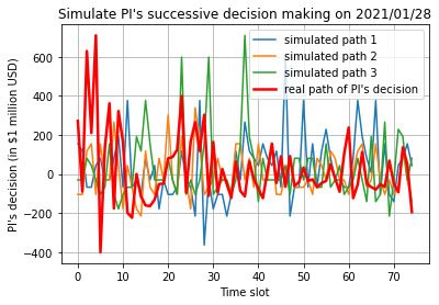
2

[25], [26] to explain the approximately positive correlation            We define PI as the aggregation of investors who are
between the stock price change and PI’s decision: a single           considered as the dominating force in the equity market. PI
retail investor easily believe that the instantaneous observation    could be composed of large institutional investors or a sizable
of PI’s decision is the most investors’ concurrent decision          group of retail investors acting in concert. PI’s decision is
to follow. Leader-follower type Keynesian beauty contest             concerned with the amount of money flowing into or out of
discloses the behavior pattern of a single retail investor but not   a stock within a time slot. We approximately quantize PI’s
PI’s strategy to make decision that is also the last remaining       decision as a signed number d ∈ Ωd in terms of the opening
piece of our MDP. In contrast to conventional MDP that               price o ∈ Ωo , the highest price h, the lowest price l, the closing
associates a single type of factor (i.e., state) to the action       price c ∈ Ωc , and the volume v:
selection by a policy function, we believe that the action
selection depends on two types of factors (i.e., visible state                                  h−o
                                                                                      d = vh             sign (c − o).               (1)
and hidden state) and build a visible-hidden Markov network                                     h−l
to model the dependency of PI’s decision making on visible           This representation allows the difference between the opening
factor and hidden factor. An algorithm is proposed to update         and closing prices to indicate the direction of the money flow.
the visible-hidden Markov network for best possibly fitting the      Moreover, the difference between the opening and highest
visible state sequence and the observation sequence. Through         prices becomes a primary determinant of the money flow vol-
the instrumentality of a trained visible-hidden Markov network       ume. Through simple math deduction, this synthetic variable
for imitating PI’s behavior from observations, we simulate the       is proved to have a monetary unit, and we consider it as USD
paths of PI’s successive decision making and further transform       in this paper.
them to stock price paths through Bayesian inference and                The sample spaces Ωd and Ωo (or Ωc ) constitute respec-
regression analysis. Imitation by means of our visible-hidden        tively the MDP action space and state space. The price change
Markov network is proved experimentally a robust approach to                                           c
effectively process the input signal with low Signal-to-Noise                                    g = −1                            (2)
                                                                                                       o
Ratio (SNR), so it is particularly suitable for the financial        functions as an indicator of the MDP state transition. We
fields. Imitation learning has become a hot topic in robotics        presume that the price change is incompletely impacted by
research. However, some imitation learning algorithms in             PI’s decision and partly random. This implies that the price
robotics, such as maximum entropy based Inverse Optimal              change follows a probability distribution which is dependent
Control (IOC) [16], [17], [18] and imitation learning from           on PI’s decision. We intend to use a data-driven regression
state observation without action information [19], require           method to determine this probability distribution and verify
demonstration samples with high SNR and are not easy to              our presumption. For this aim, we resort to B-DNN [10], [11],
be applied to financial scenarios.                                   [12], [13] which applies Bayesian statistics to DNN weights
   The final step in reaching our ultimate goal is designing an      inference. By further merging B-DNN with Gaussian process
optimization criterion for pricing the option and a dynamic          [20], [21], the price change distribution is simplified as a
hedging algorithm that can efficaciously take advantage of           gaussian distribution.
the cross-sectional information yielded by simulated price                                                   T−1
                                                                        Given a dataset D := {(dn , gn )}n=0 which contains pairs
paths of the underlying stock. To this end, a self-financing         of quantized PI’s decision and the price change sampled
portfolio is built to dynamically replicate the option price.        from T consecutive time slots, we apply Stochastic Gradient
The self-financing restriction raises a risk of exhausting cash      Descent (SGD) coupled with the dataset D to train a DNN.
for rebalancing the portfolio during the life of the option          The DNN takes an input data dn and returns a predicted
owing to a volatile price of the underlying stock. With the          value fθ (dn ) ∈ R to compare with the observed value cn
intention of minimizing this risk, the option price is comprised     for producing the empirical loss, where θ = [θ1 , . . . , θM ]
                                                                                                                                     T
of a risk-free price and a risk-adjustment. The self-financing       signifies the DNN weights. The loss is defined in terms of the
restriction also guarantees that the portfolio’s value change        loss function l (gn , fθ (dn )) and the L2 regularizer r (θ) with
between adjacent time steps comes from the portfolio’s return.       a regularization parameter λ:
Thus, we are capable of exploiting reinforcement learning to
maximize the cumulative risk-adjusted return for recursively                    L (θ, D) = L (θ, D) + r (θ)
learning the hedging position and pricing the option.                                          T−1
                                                                                               X                           λ T
                                                                                           =         l (gn , fθ (dn )) +     θ θ.   (3)
                                                                                               n=0
                                                                                                                           2
   II. E FFECT OF THE PRINCIPAL INVESTOR ’ S DECISION
                                                                        In contrast to fit a point estimate of DNN weights, B-DNN
   As described in the introduction section, we are motivated        learns a distribution over the weights. We take advantage of
to model the evolution of the underlying stock price by              this merit of B-DNN to infer the posterior distribution over the
virtue of DNN and behavioral analysis, rather than analytically      weights (Bayesian inference) and therefrom derive a posterior
characterize stochastic processes in traditional way. With this      predictive distribution which measures the distribution over
end in view, a non-deterministic MDP is designed to associate        price change induced by PI’s decision (Regression analysis).
stock price evolution with PI’s successive decision making.             In order to implement Bayesian inference on the weights,
This section is on a quest for the impact of PI’s decision on        the loss is straightforwardly embedded in the posterior dis-
stock price change.                                                  tribution over the weights via the exponential family form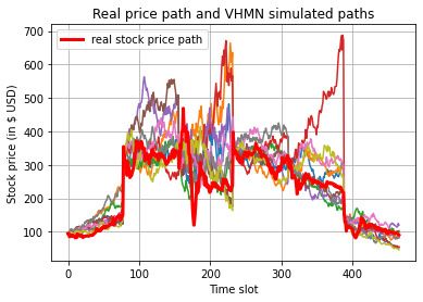
3
−L (θ,D)
P (θ | D) := R ee−L (θ,D) dθ . It implies both the likelihood
and the prior also belong to the exponential family with
−L(θ,D)
the expression as P (D | θ) := R ee−L(θ,D) dθ and P (θ) :=
−r (θ,D)
R e .
In such a manner, the Maximum A Posteriori
e−r (θ,D) dθ
b = arg max P (θ | D) is equivalent to
(MAP) estimation θ
θ
minimize mean square error. However, the immediate MAP
estimation is often computationally impractical.
Laplace approximation [22], [23], [24] provides a compu-
tationally feasible Bayesian inference on weights. The main (a) (b)
idea is to approximate likelihood times prior with a Gaussian
density function in respect that likelihood times prior is a
well-behaved uni-modal function in L2 space. The posterior
distribution over the weights is consequently derived to be the
below Gaussian distribution (see derivation in Appendix A):
−1
P (θ|D) ≈ N θ | θ ∗ , ∇2θθ L (θ ∗ , D) + λIM
, (4)
T
where θ ∗ = [θ1∗ , . . . , θM
∗
] is the mode of P (D | θ) P (θ).
After obtaining the posterior over the weights, we then
seek for the posterior predictive distribution over price change
(c) (d)
P (g ∗ | d∗ , D), where d∗ ∈ R denotes a test sample of
quantized PI’s decision and g ∗ signifies the corresponding ob-
servation of the price change. The high dimensional projection
and the nonlinear relationship between d∗ and fθ∗ (d∗ ) impede
to directly find P (g ∗ | d∗ , D) in closed form. In order to
overcome this impediment, a new random variable y which
has a readily accessible posterior predictive distribution is
constructed and can be linearly expressed in terms of g ∗ . As
a result, P (g ∗ | d∗ , D) is inferred from the given posterior
predictive distribution P (y | d∗ , D). As presented in [20],
y is possible to be designed as a linear combination of a (e) (f)
Gaussian process and additive gaussian noise. Different from
Figure 1: GME behavior observed in each 5-minute time slot
[20], we calculate the parameters of the Gaussian process (i.e.,
from 09:35 to 16:00 during 6 consecutive trading days. Earlier
m (d∗ ) in Equation (8) and k (d∗ , d∗ ) in Equation (9)) based
T−1 time slots are with lighter shades.
on P (θ|D) instead of P (θ|D 0 ) where D 0 := {(yn , cn )}n=0
is a transformed dataset and yn is a sample of the constructed
variable. In addition, we consider the residual (ε in Equation
(7)) as additive independent identically distributed (i.i.d) Gaus- As the linear regression model is built on the feature space in
sian noise rather than additionally bring in the second-order Equation (6), it successfully leaves the difficulty of processing
partial derivatives of the loss to represent noise. non-linear high-dimensional mapping back to DNN.
The random variable y is designed as the following com- For a quadratic loss function l (g ∗ , fθ∗ (d∗ )) =
1 ∗ ∗ 2
bination of the standard linear regression model and the first 2 (g − f θ ∗ (d )) , the constructed random variable y
order derivative of the loss function: can be simplified in terms of g ∗ from Equation (5):
T
y = φ (d∗ ) θ + ∇fθ∗ (d∗ ) l (g ∗ , fθ∗ (d∗ )) , (5)
T
where DNN weights follow a prior distribution θ ∼ y = φ (d∗ ) θ + (fθ∗ (d∗ ) − g ∗ )
N (0, Kθθ ) with the covariance matrix Kθθ = λ−1 IM . And = ϕ (d∗ ) + ε, (7)
φ (d∗ ) is a Jacobian matrix whose entries form a set of basis
functions to project the input sample into M dimensional where fθ∗ (d∗ ) − g ∗ is the residual that can be modeled
feature space: as additive independent
identically distributed Gaussian noise
ε ∼ N 0, σ 2 . Gaussian process is an effective tool for de-
scribing a distribution over functions [21]. From the function-
φ (d∗ ) = ∇θ fθ (d∗ ) |θ=θ∗
∂f (d∗ ) space view, the process ϕ (d∗ ) is specified by a Gaussian pro-
θ
∂θ1 | θ=θ1∗ cess ϕ (d∗ ) ∼ GP (m (d∗ ) , k (d∗ , d∗ )), where we calculate the
=
.
..
, (6) mean function m (d∗ ) and the covariance function k (d∗ , d∗ )
based on the posterior distribution over the weights P (θ|D)
∗
∂fθ (d )
∂θM |θM =θM∗
obtained in Equation (4):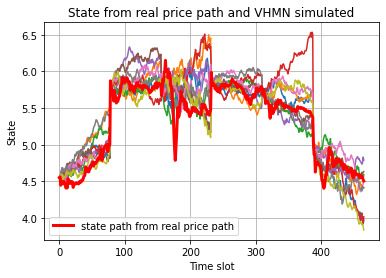
4

                                      T
                     m (d∗ ) = φ (d∗ ) E [θ | D]
                                      T
                            = φ (d∗ ) θ ∗ ,                     (8)

                            h         i
                        T
  k (d∗ , d∗ ) = φ (d∗ ) E θθ T | D φ (d∗ )
                                                −1                                  (a)                               (b)
                        T
               = φ (d∗ ) ∇2θθ L (θ ∗ , D) + λIM     φ (d∗ ) . (9)
  Equation (7) exhibits that the random process y is a linear
combination of a Gaussian process and additive Gaussian
noise. Therefore, the posterior predictive distribution of y
can be easily deduced from the statistical description of the
Gaussian process and Gaussian noise as:

                                                                                   (c)                               (d)
                              T
    P (y | d∗ , D) = N φ (d∗ ) θ ∗ , k (d∗ , d∗ ) + σ 2 .      (10)

    Since we always prefer to perform a prediction based on
the DNN weights at the mode of the posterior θ ∗ rather than
any possible DNN weights, only the determinate realization
        T
φ (d∗ ) θ ∗ should be extracted from the Gaussian process in-
                                             T
stead of the entire Gaussian process φ (d∗ ) θ for calculating
g ∗ . Thuswise g ∗ is a linear combination of a random variable
and a constant:                                                                      (e)                               (f)

                                                                             Figure 2: Regression with σ = 2.5 and λ = 0.7
                 ∗              ∗ T   ∗            ∗
                g = y − φ (d ) θ + fθ∗ (d )
                     = y + C.                                  (11)   period from 09:35 to 16:00 for the 6 consecutive trading days.
  Consequently, the posterior predictive distribution over price      Each sample is a five-dimensional vector which enumerates
change is derived from Equation (10) and (11):                        open-high-low-close prices and volume observed in a 5-minute
                                                                      time slot. We discard the pricing data in the first time slot
                                                                      (i.e., 09:30 to 09:35) because the open price is subject to the
     P (g ∗ | d∗ , D) = N fθ∗ (d∗ ) , k (d∗ , d∗ ) + σ 2 .

                                                               (12)   pre-market trading and gaps up or down from the previous
                                                                      day’s close. Moreover, the volume in the first time slot is
   The observation of the price change g ∗ shares the same
                                                                      extremely high and influenced by the pre-market news. Based
posterior predictive variance with y owing to the fact that
                                  T                                   on Equation (1), (2) and dataset D, we yield the training
the predicted value φ (d∗ ) θ ∗ is a determinate realization                                       Ti −1
                                                                      dataset Di := {(dn , gn )}n=0      which contains the pairs of
produced at the mode of the posterior θ ∗ and the deduction
                                                                      quantized PI’s decision and price change sampled from Ti
of the predicted value from y is incapable of eliminating the
                                                                      consecutive time slots in the ith episode as illustrated in Figure
immanent uncertainty in the inference on weights and the
                                                                      1. The samples are plotted in chronological order. The lighter
residual. When we consider an input vector of test samples
                        T                                             shade indicates that the sample is taken in an earlier time slot.
d∗ =[d∗1 , . . . , d∗N ] , Equation (12) turns into the below form:
                                                                          We first train B-DNN respectively on an episode basis
                                                                      with the training dataset Di,i=1...6 to determine the posterior
 P (g ∗ | d∗ , D) = N fθ∗ (d∗ ) , diag k (d∗ , d∗ ) + σ 2 IN

                                                             .        distribution over the weights and then work out the posterior
                                                           (13)       predictive distribution over price change led by testing samples
   During Jan. 26, 2021-Feb. 02, 2021, GameStop Corporation           of quantized PI’s decision. The testing samples are produced
(GME) stock price swiftly rose and then fell with the unusually       to be evenly spaced over the interval between the largest and
high price and volatility because a short squeeze was triggered       smallest training sample of quantized PI’s decision in each
by organized retail investors. We would like to explore the           episode. There are two fine-tuned hyperparameters σ and λ for
behavioral finance behind this event through our model. The           optimizing our model’s performance. Since σ has a significant
intraday data for the 6 consecutive trading days is exercised         influence on posterior predictive variance as shown in Equation
to infer B-DNN coefficients and be referred to produce testing        (12), the optimal value of σ can be found out by the "68–95–
samples for validating regression analysis. Due to the unreach-       99.7 rule". We carry out Bayesian inference and regression
ability, the pre/post-market data is not included even though         analysis with two sets of parameters (σ = 2.5, λ = 0.7,
some huge price fluctuations occurred in the pre/post-market          and σ = 1, λ = 0.1) and exhibits the results in turn by
sessions. We structure a dataset D as 77 samples in each              Figure 2 and Figure 3. It is observed that σ = 2.5 offers a
of 6 episodes to accommodate the equity pricing data in the           fitting posterior predictive variance to satisfy in principle the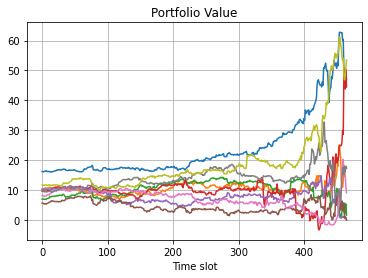
5

               (a)                              (b)
                                                                              Figure 4: Visible-hidden Markov network

                                                                    choices and match the choice of the majority based on the
                                                                    own guess. Keynes believed that the similar behavior pattern
                                                                    applies to the investors within the stock market. Most investors
                                                                    attempt to make the same decision that the majority do rather
               (c)                              (d)                 than build a decision on their own evaluation of fundamental
                                                                    profitability. However, it is very hard to guess other investor’s
                                                                    concurrent decision for a retail investor. For this reason, the
                                                                    stock market evolves into a leader-follower type Keynesian
                                                                    beauty contest where a single retail investor (i.e., follower)
                                                                    tends to follow the instantaneous observation of PI’s decision
                                                                    and thinks it as the most investors’ concurrent decision. The
                                                                    leader-follower type Keynesian beauty contest explains well
                                                                    the approximately positive correlation between PI’s decision
               (e)                              (f)
                                                                    and the stock price change. Nevertheless, PI’s decision making
          Figure 3: Regression with σ = 1, λ = 0.1                  is still inadequate to be inferred from the leader-follower type
                                                                    Keynesian beauty contest.
                                                                       We believe that two types of factors influence PI’s decision
"68–95–99.7 rule", while σ = 1 leads a too small posterior          making: visible and hidden. The visible factor is observable,
predictive variance to match the actual data distribution. The      while the hidden factor is hard to be quantized or detected,
experimental evaluation also demonstrate that the overfitting       for example, the impact of news on investors’ anticipation of
is effectively prevented by λ. As shown in Figure 2, the            the investment return and thus on their investment behavior.
overfitting is fully suppressed by a relatively large regular-         The conventional MDP applies a policy function to map
ization parameter λ = 0.7. On the other hand, overfitting           state space to action space. However, the policy function is
emerges when the regularization parameter decreases to a            not sufficient for mapping two state spaces to action space.
smaller value, for instance, λ = 0.1 as illustrated in Figure 3.    In order to identify the dependency of PI’s decision making
Furthermore, we can observe from the numeric results that the       on visible factor and hidden factor, we build a visible-hidden
stock price change has an approximately positive correlation        Markov network as shown in Figure 4. The hidden factor
with quantized PI’s decision.                                       is modeled by a random variable (i.e., hidden state) which
                                                                    changes through time and the visible factor is modeled by
 III. I NVERSE PI’ S DECISION FROM VISIBLE AND HIDDEN               another random variable (i.e., visible state). The hidden state
                            STATES                                  transits over time slots, and its transition is a Markov process.
   The previous section presents a DNN-based approach to de-        In the same time slot, the hidden state, the visible state, and the
termine the state transition (i.e., price change) after executing   random variable representing PI’s decision (i.e., observation)
an action (i.e., principal investor’s decision). We still wonder    are pairwise correlated. We design a chain for connecting these
how an action is made and especially how associate an action        random variables to enable the calculation of the dependencies
with the current state (i.e., open price). Answering this query     among them. This chain design differentiates the visible-
equals the proffer of the last remaining piece of our MDP.          hidden Markov network from hidden Markov models [27]
This section will find out the underlying law to simulate PI’s      which considers only two coinstantaneous components without
successive decision making.                                         the visible state. In each time slot, the hidden state is directly
   When we ground the numerical results on the real equities        connected to the visible state and then indirectly chained to
pricing data in the previous section, it is observed that higher    the observation via the visible state.
quantized PI’s decision approximately leads to higher stock            We specify the notations used in the visible-hidden Markov
price change. This phenomenon can be theoretically explained        network below:
by the Keynesian beauty contest [25], [26]. Keynesian beauty           ζ = {ζ0 , ζ1 , . . . , ζJ−1 }: hidden state sample space,
contest describes a beauty contest where voters win a prize for        ν = {ν 0 , ν1 , . . . , νK−1 }: visible state sample space,
voting the most popular faces among all voters. Under such             ω = {ω0 , ω1 , . . . , ωL−1 }: observation sample space,
rule of the contest, a voter tends to guess the other voters’          Z = {z0 , z1 , . . . , zJ−1 }: initial hidden state distribution,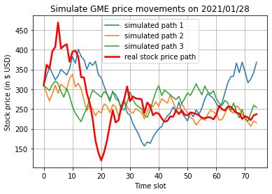
6

   A = {aij } ∈ RJ×J : hidden state transition matrix,
   aij = P {hidden state ζj at t + 1 | hidden state ζi at t},
   B = {bi (k)} ∈ RJ×K : visible state probability matrix,
   bi (k) = P {visible state vk at t | hidden state ζi at t},
   C = {ck (l)} ∈ RK×L : observation probability matrix,
   ck (l) = P {observation ol at t | visible state vk at t},
   H = {h0 , h1 , . . . , hT−1 }: hidden state sequence,
   S = {s0 , s1 , . . . , sT−1 }: visible state sequence,
   O = {o0 , o1 , . . . , oT−1 }: observation sequence,
   Γ = {A, B, C, Z}: Visible-hidden Markov network.                                                      (a)                                          (b)
   In our scenario, the hidden state indicates bullish or bearish
news received just before a time slot, so the hidden state                             Figure 5: Simulation of PI’s successive decision making
sample space ζ is with a size of 2. The visible state and
the observation chained to the same hidden state represent
respectively the opening price and quantized PI’s decision in
the same time slot influenced by the just acquired market
information. The visible state sample space ν and the ob-
servation sample space ω are finite and discrete compared
with the continuous sample space of the opening price and
quantized PI’s decision. For this reason, we borrow the concept
of the quantization in digital signal processing to map values
from the sample space of the opening price and quantized PI’s
decision to ν and ω:                                                                                     (a)                                          (b)

                                      s                                                      Figure 6: Simulation of GME price movements
                           s = b smax −smin c,                                (14)
                                         Q

where bc is the floor function. s stands for a sample value
of the opening price or quantized PI’s decision. smax and
smin mark respectively the upper and lower limits of the                                                                                           βt0 (i) = P (s0 , s1 , . . . , st , o0 , o1 , . . . , ot , ht = ζi |Γ)                                            X
                   K−1                                                                                             =         γt (i, j) .                     (21)
                   X
                                                                                                                       j=0
               =         αt−1 (j) aji bi (st ) cst (ot ) ,                    (16)
                   j=0                                                                 Step 3: Re-estimate Γ:

    βt=T−1 (i) = P (sT−1 , oT−1 |hT−1 = ζi , Γ) = 1,                          (17)                                 zi = γt=0 (i) ,                           (22)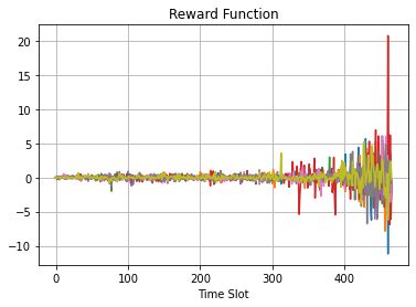
7
PT −2 of B-DNN inference-regression presented in the section II,
t=0 γt (i, j) likely evolutionary paths of PI’s decision are transformed into
aij = PT −2 , (23)
t=0 γt (i)
probable price paths of the underlying stock. These simulated
P price paths of the underlying stock yield the cross-sectional
t∈{0,1,...,T −1},st =ν k γt (i)
bi (k) = PT −1 , (24) information for optimizing a dynamically hedged portfolio.
t=0 γt (i) This section expounds how to reinforcement learn option price
using the cross-sectional information stemmed from imitative
P
t∈{0,1,...,T −1},st =ν k ,ot =ωl γt (i)
ck (l) = PT −1 . (25) PI’s chronological decision making.
t=0 γt (i) Suppose that we sell a European option with the terminal
PJ−1
Step 4: If P (S, O | Γ) = i=0 αt=T−1 (i) climbs, go to payoff H (ST ), where ST denotes the underlying stock price at
Step 2, otherwise end the loop. expiry date T. For the sake of the suitability of our algorithm
The parameters of a visible-hidden Markov network is ini- for both calls and puts, switching the below expression of the
tialized before entering the iterative process and then updated terminal payoff will turn pricing/hedging a call option into a
in each iteration until P (S, O | Γ) doesn’t grow anymore. put option:
A, B, C, and Z are row stochastic, moreover, their rows (
max (ST − K, 0) , if calls
respectively belong to a standard J −1, J −1, K −1, and L−1 H (ST ) = (26)
simplex which are the support of the Dirichlet distribution of max (K − ST , 0) , if puts.
order J − 1, J − 1, K − 1, and L − 1. Therefore, we can With the proceeds from the sale of the option, we build
employ the Dirichlet distribution to randomize A, B, C, and a portfolio Πt which consists of at units of the stock with
Z to keep away from a local maximum which prevents the price St and a deposit in the risk-free bank account Bt . With
evolution of the model. the aim of dynamically hedging the option, we rebalance this
Figure 1c and 1d clearly show that PI’s decision making portfolio to keep its value replicating the value of the option
strategy varies from one episode to another: PI preferred to at time t 6 T:
give a decision with large absolute value at the early stage
on Jan. 28, 2021, on the other hand, tended to spread large Πt = at St + Bt . (27)
trades over time on Jan. 29, 2021. In light of this signs,
our determination of a visible-hidden Markov network is At maturity we close out the position as we no longer need
episode-based. We measure Γ in each episode to generate time hedge the option. Consequently, the terminal payoff is the
series of the probable evolution of PI’s decision making and portfolio value at maturity:
further transform them to stock price paths through Bayesian
inference and regression analysis. ΠT = H (ST ) = Bt (28)
We imitate PI’s successive decision making based on obser- We ignore transaction costs or other frictions in this paper
vations from the training dataset Di,i=1...6 . The hyperparame- due to the fact that low rates or fixed commissions are offered
ters are given the following values: J = 2, and K = L = 30. to the customers with high volume of trades executed (e.g.,
We parametrize Dirichlet distribution with αi = 1000, so High-Frequency Trading (HFT) firms). We force our dynami-
that the initial A, B, C, and Z are row stochastic and have cally hedged portfolio Πt to be self-financing in such a manner
near uniform values, where αi denotes any component of the that there is no external infusion or withdrawal of cash over
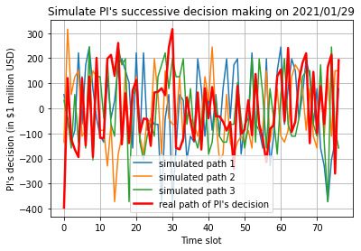
parameter vector α. Figure 5 exhibits three simulated paths of the lifetime of the option, and the spread of portfolio values
PI’s successive decision making along with the real evolution at different times comes from the continuously compounded
of PI’s decision. In view of article space, we only show risk-free interest rate r and the change in underlying stock
the experimental results in two representative episodes for price 4St :
comparison in figures. According to Figure 5a and 5b, we find
that the simulated paths on Jan. 29, 2021 are more volatile than Πt+1 − er Πt = at 4 St + κfθ∗ (F ) at St , (29)
those on Jan. 28, 2021. This correctly reflects the discrepancy
of the volatility of real PI’s decision on these two days and thus where 4St = St+1 − er St and F = (at+1 − at) ΘSt .
well proves the effectiveness of our algorithm. The B-DNN The cross-sectional information F (t) = St1 , . . . , StU
is trained by the training dataset Di,i=1...6 when we perform collects possible prices at time t from all the simulated
Bayesian inference in the section II. We continue to carry out price paths, where U is the number of simulated paths and
regression analysis grounded on this trained B-DNN for each Stu ,u=1,...,U denotes the price at time t sampled from the
evolutionary path of PI’s decision. For the sake of simplicity, uth path. Our cross-sectional information is derived from
the price change is simulated as its posterior predictive mean. the existing PI’s decision, so we design an compensation
Figure 6 illustrates our simulated price movements of the term κfθ∗ (F ) at St to put in the price change caused by our
underlying stock together with the real price path. hedging activity if we are also referred to as PI. fθ∗ (F )
maps a large-scale volume of buying or selling the underlying
IV. R EINFORCEMENT LEARN OPTION PRICE GROUND stock to a sharp rise or drop in price via our trained B-DNN.
UPON IMITATIVE PI’ S CHRONOLOGICAL DECISION MAKING We may sell multiple options covering significant amount of
Our algorithm introduced in the section III probabilistically shares of the underlying stock. We use Θ to denote the total
imitates PI’s chronological decision making. With the help number of shares of the underlying stock. The coefficient κ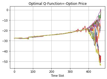
8
gives a degree of freedom to scale the compensation term.
If we are a single retail investor who sells a mini option, Πt = Πt Set , (36)
then this compensation term vanishes as κ tends to 0. Monte
Carlo sample-based reinforcement learning [28] uses the cross- where π is the policy function which maps Set and t to the
sectional information which is generated by sampling a pre-set position in the stock at time t.
probability distribution. Compared with Monte Carlo sample- We are aiming to find a policy to price the option with the
based reinforcement learning, our algorithm can better fit into satisfaction for the only necessary demand of hedging risk, or
each circumstance as we adopt the cross-sectional information other kind of statement, catch the optimal
or nearly optimal
that reflets the existing PI’s decision and add an compensation π that minimizes the ask price Ct Set . Our goal can be
term to compensate the effect of our hedging activity on the achieved by using reinforcement learning which translates the
price change. aim into learning π that maximizes the expected cumulative
When price an option at any time within its lifetime, the risk reward via maximizing the state-value function and the action-
of running out cash to continue rebalancing the portfolio due value function [30]. Reinforcement learning is found on a
to the fluctuation in the market price of the underlying stock MDP. In our scenario, the stock price Set ∈ S is the state and
should be taken into account. To this end, the ask price Ct at the position in the stock e at ∈ A is the action. Accordingly,
time t 6 T is designed to be the sum of the risk free price and the sample space of the stock price S and the position A
the risk-adjustment weighted by the risk-aversion coefficient respectively form the state space and the action space. The
η [28] as expressed in Equation (30). The risk free price is function for a policy π at time t is denoted as
state-value
the expected value of the portfolio Πt . The risk-adjustment Vtπ Set and it is designed as the negative of the option
accumulates the risk from time t until the expiry date T. The
price. Equation (29) formulates the chronological recursive
risk at time t is quantized as the expected discounted variance
relationship that expresses the portfolio’s value at time t in
of the portfolio Πt .
respect of its value at the subsequent time t+1. We can exploit
" # this chronological recursive relationship to find the Bellman
T
X
−r (t0 −t) equation for the state-value function and the reward:
Ct (St ) = Et Πt + η e Var [Πt0 | Ft0 ] |Ft .
t0 =t
(30) Vtπ Set = −Ct Set
Geometric Brownian motion is the most commonly used
model of stock price behavior. By applying Itô’s lemma to (37)
the random variable of stock price which follows Geometric " T
#
Brownian motion, the stock price at time t is proved to be −r (t0 −t)
X
= Et −Πt − η e Var [Πt0 | Ft0 ] |Ft
lognormally distributed [29]: t0 =t
(38)
σs2
2
ln St ∼ N ln S0 + µ − t, σs t ,
" #
(31) T
2 −r (t0 −t)
X
= Et −Πt − ηVar [Πt0 ] − η e Var [Πt0 | Ft0 ] |Ft
where µ is the expected rate of return per time-slot from the t0 =t+1
stock, and σs is the volatility of the stock price. (39)
h
i
Equation (31) implies St is not martingale due to the = Et Rt Set , e π
at , Set+1 + γVt+1 Set+1 ,
σ2
constant drift rate µ − 2s . When price the option, we prefer
(40)
the calculation to be based on an independent variable without
constant drift. Therefore, we expand the independent variable Equation (38) is obtained by plugging Equation (30) into
St in Equation (27), (29), and (30) to a function in terms of Equation
(37). Equation (40) is the Bellman equation for
an independent variable without constant drift Set : Vtπ Set , where the reward Rt Set , e
at , Set+1 is derived as
below by using the chronological recursive relationship given
σ2
St = exp Set + µ − s t . (32) in Equation (29):
2
St afterwards will signify the expansion of stock price in terms
of Set in all equations. Rt Set , e at 4 St + κfθ∗ (F ) St ) − ηVar [Πt | Ft ]
at , Set+1 = γ (e
The following notations will denote for short the other at 4 St + κfθ∗ (F ) St )
= γ (e
variables which are dependent on Set in subsequent derivations: 2
2
− ηγ Et Π̇t+1 − e at 4 Ṡt + κfθ (F ) e
∗ at Ṡt ,
at = e
e at Set = at , (33) (41)
where γ = e−r is the discount rate, Π̇t+1 = Πt+1 − Πt+1 ,
π = π Set , t = e
at , (34)
4Ṡt = 4St − 4S t , Ṡt = St − S t , and (·) denotes the sample
mean. Maximizing the reward is identical to maximize the
cumulative risk-adjusted return as the last term of the reward
2 2
et+1 + µ− σs (t+1)
S et + µ− σs t
S
2 r 2
4St = e −e e , (35) stands for the risk at time t and the first term quantizes the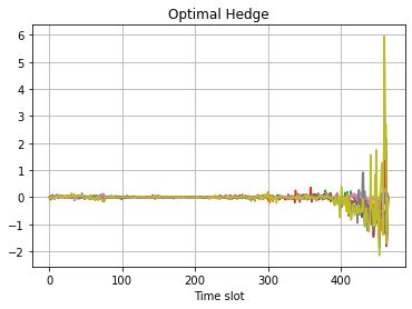
9
portfolio’s return between time t and t + 1. When η tends to In our scenario, the state space and the action space are
infinity, the hedge becomes a pure risk hedge. both continuous. We adopt basis functions, for example basis-
The action-value function (Q-function) returns the value splines, as an intermediary for mapping two continuous spaces.
of taking action a in state s under a policy π at time t. A state sample Set is first mapped to a set of basis functions and
Consequently, Q-function can be interpreted as a state-value the optimal action ea∗t is then expressed as a linear combination
∗
function under the condition of Set = s and e
at = a: of basis functions weighted by the optimal coefficients wnt :
XB
∗ ∗
h i
Qπt (s, a) = Et −Πt | St = s, e
e at = a a
et = wnt ψn Set , (47)
" T # n=1
X
−r (t0 −t) where B represents the number of basis functions. Similarly,
− Et η e Var [Πt0 | Ft0 ] |St = s, e
e at = a .
the optimal Q-function value can be formulated as a linear
t0 =t
(42) combination of basis functions weighted by the optimal coef-
∗
ficients ϕnt :
∗
We use Qπt Set , e a∗t to stand for the Q-function value X B
which is maximized by the optimal policy π ∗ which chooses ∗
a∗t =
Qπt Set , e ϕ∗nt ψn Set . (48)
the optimal action ea∗t in state Set at time t: n=1
Our objective of finding optimal policy and Q-function
value is consequently transformed into learning the optimal
∗
Qπt a∗t = maxQπt Set , e
Set , e at ∗
π
coefficients wnt and ϕ∗nt . We elaborate the derivation of the
∗
= max Qπt Set , e
at , (43) following closed-form solution of wnt in Appendix B:
at ∈A
e
wt∗ = E−1
t Dt , (49)
where π ∗ = π ∗ Set , t and e
a∗t = e
a∗t Set are both dependent
on Set .
B
U
" #
The Bellman optimality equation for the action-value func- t
X X
Enm = ψm Setu 4 Ṡt Ξ ψn Setu
tion has a similar structure to the Bellman equation for the
u=1 n=1
state-value function (Equation (40)) and can be expanded by U
" B
#
plugging Equation (41) into it:
X X
+ κfθ∗ (F ) ψm Setu Ṡt Ξ u
ψn Set , (50)
u=1 n=1
Qπt
Set , e
at U
" B #
X 4Stu κfθ∗ (F ) Stu X
h ∗
i Dnt = + Π̇t+1 Ξ + u
ψn St ,
a∗t+1
e
=Et Rt Set , eat , Set+1 + γQπt+1 Set+1 , e (44) 2ηγ 2ηγ
u=1 n=1
h ∗
i (51)
=γEt eat 4 St + κfθ∗ (F ) e a∗t St + Qπt+1 Set+1 , ea∗t+1
Ξ = 4Ṡt + κfθ∗ (F ) Ṡt , (52)
2
2
− ηγ Et Π̇t+1 − e at 4 Ṡt + κfθ∗ (F ) e
at Ṡt .
where wt∗ is a B-dimensional vector with entry wnt ∗
, Et is
(45) t
a matrix of size B × B with entry Enm and Dt is a B-
The terminal condition gives the optimal Q-function value dimensional vector with entry Dnt . We can also introduce a
at expiry in terms of the terminal payoff: regularization parameter ς with a very small value as Et +ςIB .
∗
This regularization parameter prevents Et from becoming a
a∗T = −H (ST ) − Var [H (ST )] ,
QπT SeTu , e (46) singular matrix which does not have an inverse.
Once we obtain the optimal action e a∗t from Equation (49)
where e a∗T = 0. and Equation (47), the optimal Q-function value at time t can
Our purpose is to find π ∗ Set , t or e a∗t Set , and be inferred by an expectation in terms of the reward at time
∗
t and the optimal Q-function value at time t + 1 through the
Qπt Set , e a∗t . However, the unknown value of Set and the
Bellman optimality equation (Equation (44)) at the optimal
incalculable expectation in the Bellman optimality equation a∗t . However, in practice we take the sample from our
action e
prevents us from achieving our goal. For the removal of simulated path instead of the expectation to infer the optimal
the barrier,
n o we use the cross-sectional information Fe = Q-function value at time t and this will produce error eu which
u
St
e to take as many likely values of Set into is the deviation of the observed value from the true value:
u=1,...,U
σ2
account as possible, where Setu = ln Stu − µ − 2s t. We h i
∗ ∗
believe that our simulated price paths have the same constant Qπt a∗t = Et Rt Set , e
Set , e a∗t+1
a∗t , Set+1 + γQπt+1 Set+1 , e
drift as those follows a lognormal distribution. Moreover, the ∗
incalculable expectation in the Bellman optimality equation is a∗ , Seu
= Rt Seu , e t t + γQπ
t+1 a∗
Seu , e + eu .
t+1 t+1 t+1
approximated by an empirical mean of U observations. (53)10
The optimal Q-function value at time t can be learned by
reaching the criteria of minimizing the sum of squared errors
in all simulated paths:
U
X
ϕ∗nt = min e2u
ϕnt
u=1
U B
!2
X X
= min Fu − ϕnt ψn Setu , (54)
ϕnt
u=1 n=1
(a) (b)
∗
where Fu = Rt Setu , e a∗t , Set+1
u
+ γQπt+1 Set+1
u
a∗t+1 .
,e
The optimal coefficients ϕ∗nt is approximated by the least Figure 7: Imitative GME price movements
b∗t :
square estimator ϕ
ϕ∗t ≈ ϕ
b∗t
= G−1
t Ht , (55)
Gtnm = ψn Setu ψm Setu , (56)
∗
Hnt = ψn Setu Rt Setu , e a∗t , Set+1
u
+ γQπt+1 Set+1
u
a∗t+1 ,
,e
(57)
where ϕ∗t is a B-dimensional vector with entry ϕ∗nt , Gt is (a) (b)
a matrix of size B × B with entry Gtnm and Ht is a B-
dimensional vector with entry Hnt .
We are ultimately able to predict the option price Ct Set =
∗
−Qπt Set , ea∗t and the hedge position e a∗t backward recur-
sively at any time until the expiration date by triggering the
following algorithm:
Algorithm of learning option price and hedge position
∗
1: Calculate Qπ eu , e
S ∗
T T aT with Eq. (46) and ΠT with Eq. (28)
2: for t = T − 1 to t = 0 do (c) (d)
3: Calculate wt∗ with Eq.(49), a∗t with Eq. (47) and Πt with Eq. (29)
e
Figure 8: Reinforcement learn option price and hedging posi-
4: Calculate Rt S a∗t , S
et , e et+1 with Eq. (41)
tion ground upon imitative PI’s chronological decision making
∗
∗
5: Calculate ϕt with Eq.(55) and Qπ S a∗t with Eq. (48)
et , e
t
6: end for
7a. We remove the constant drift from all the prices paths and
V. E XPERIMENTAL E VALUATION plot the real state Set and the simulated states Setu in Figure 7b.
We evaluate our entire algorithm/process on a task of The drift rate is calculated with µ = 0.05 and σs = 0.2926.
hedging and pricing a European call option based on 100 The value of σs is derived from averaging the daily VIX index
shares of the underlying GME stock with a period of 6 from Jan. 26, 2021 to Feb. 02, 2021. The total number of
trading days and a strike price of 100 USD. Suppose that the simulated paths is 1000 and only 10 paths are uniformly
we have learned that the leading investors are the same group sampled to be shown here. The training samples are sampled
of investors who took on the role as PI during Jan. 26, 2021- in each 5-minute time slot. The simulated paths are also with
Feb. 02, 2021. Therefore, our first step is to probabilistically a time resolution of 5 minutes. The price jumps that appear
imitate their previous successive decision making from the hid- in Figure 7a and 7b are owning to the pricing data in the first
den motives behind them through our visible-hidden Markov time slot (i.e., 09:30 to 09:35). The open price and the volume
network as we presented in the section III. The second step in this time slot deviate far from the average owing to their
is to transform likely evolutionary paths of PI’s decision into high dependence on the pre-market trading and news. For this
probable price paths of the underlying stock by our B-DNN reason, the training dataset does not include the pricing data in
inference-regression process introduced in the section II. For the first 5-min time slot, and we interpolate the real value in the
the above two steps, we train a B-DNN and a visible-hidden figures. The Visible-hidden Markov network is abbreviated to
Markov network on an episode basis with the training data set VHMN in the figures for the benefit of space. We can observe
Di,i=1...6 . The simulated price paths along with the real price that the visible-hidden Markov network produces imitative
paths used as the training data samples are compared in Figure price paths that have highly matched behavior pattern with the11
real price path. As a consequence, the visible-hidden Markov [14] Kailai Xu and Eric Darve. Calibrating multivariate lévy processes with
network is a powerful tool to cope with the intrinsic instability neural networks. In Mathematical and Scientific Machine Learning,
pages 207–220. PMLR, 2020.
in financial data by engendering imitative variations for each
[15] Olivier Pironneau, Calibration of heston model with keras,
specific scenario. https://hal.sorbonne-universite.fr/hal-02273889, 2019
Our final phase of this task is to perform the algorithm of [16] C. Finn, S. Levine, and P. Abbeel. Guided cost learning: Deep inverse
learning option price and hedge position. We rebalance the optimal control via policy optimization. In Proceedings of the 33rd
portfolio every 5 minutes during 6 trading days. The risk-free International Conference on Machine Learning, 2016.
[17] Ziebart, B., Maas, A., Bagnell, J. A., and Dey, A. K. Maximum en-
interest rate r = 1.059% is taken the average of daily US 10- tropy inverse reinforcement learning. In AAAI Conference on Artificial
year bond yield from Jan. 26, 2021 to Feb. 02, 2021. We set Intelligence, 2008.
κ = 0 as we only hedge a mini option based on 100 shares. We [18] J. Yang, X. Ye, R. Trivedi, H. Xu, and H. Zha. Learning deep mean
also give η1 = 0 for having pure risk hedge. ς = 0.001 is used field games for modeling large population behavior. arXiv preprint
arXiv:1711.03156, 2017.
to avoid the error of inversing a singular matrix. The optimal
[19] Faraz Torabi, Garrett Warnell, and Peter Stone. Behavioral cloning from
hedging position is shown in Figure (8a), where the value on observation. arXiv preprint arXiv:1805.01954, 2018.
the graph needs to be multiplied by 100 to correspond to 100 [20] Mohammad E. K., Alexander I., Ehsan A., and Maciej K., “Approximate
shares. It is exhibited that the option is more actively hedged inference turns deep networks into Gaussian processes,” Advances in
when closer to the expiration date. The value of the replicating neural information processing systems, 2019.
portfolio jumps near the maturity date and the hedging strategy [21] Rasmussen C. E. and Williams C. K. I., “Gaussian Processes for
Machine Learning,” Cambridge, MA, USA: MIT Press, 2006.
effectively protects the portfolio against the risk of running out
[22] Rue, H., Martino, S. and Chopin, N. (2009). Approximate Bayesian
of money as shown in Figure (8b). The optimal Q-function inference for latent Gaussian models by using integrated nested Laplace
value converges at -27.586 which means we better sell the approximations. Journal of the Royal Statistical Society: Series B
option at the price of 2758.6 USD as illustrated in Figure (Statistical Methodology) 71 319–392.
[23] K. Kristensen, A. Nielsen, C. W. Berg, H. Skaug, and B. Bell. TMB:
(8d). Automatic Differentiation and Laplace Approximation. Journal of Sta-
tistical Software, 70(1):1–21, 2016.
VI. C ONCLUSION [24] L. Tierney and J. B. Kadane, “Accurate approximations for posterior
In order to address the challenges posed by intrinsic low moments and marginal densities,” J. Amer. Statistical Assoc., vol. 81,
no. 393, pp. 82–86, 1986.
SNR and instability in financial data, we innovatively exploit [25] Keynes, J. M. (1936). The General Theory of Employment, Interest and
imitative cross-sectional information to reinforcement learn Money. New York: Harcourt Brace and Co.
option price and hedging position. When we turn to behavior [26] Gao, P. (2008). Keynesian beauty contest, accounting disclosure, and
finance, another challenge of identifying the leading investor’s market efficiency. Journal of Accounting Research, 46:785–807.
behavior and the stock price change comes along. To this [27] Stamp, M.: A revealing introduction to hidden Markov models.
http://www.cs.sjsu.edu/~stamp/RUA/HMM.pdf (2011)
end, we take advantage of the excellent features of B-DNN
[28] I. Halperin. QLBS: Q-learner in the Black-Scholes (-Merton) worlds.
to explore non-deterministic relations by a market data driven arXiv:1712.04609, 2017.
fashion. [29] J. Hull, Options, Futures, and Other Derivatives, 6th ed., Englewood
Cliffs, NJ, USA: Prentice-Hall, 2006.
R EFERENCES [30] Richard Sutton and Andrew Barto. Reinforcement Learning: An Intro-
duction. MIT Press, 1998.
[1] Black, F., Scholes, M., 1973. The pricing of options and corporate
liabilities. Journal of Political Economy 81, 637–654.
[2] Merton, R.C., 1976. Option pricing when underlying stock returns are
discontinuous. Journal of Financial Economics 3, 125–144.
[3] Heston, S., 1993. Closed-form solution for options with stochastic
volatility, with application to bond and currency options. Review of
Financial Studies 6, 327–343.
[4] G. E. Monahan, “State of the art—a survey of partially observable
A PPENDIX A
markov decision processes: theory, models, and algorithms,” Manage-
ment science, vol. 28, no. 1, pp. 1–16, 1982.
[5] Hornik, K., 1991. Approximation capabilities of multilayer feedforward
networks. Neural Networks 4, no. 2, 251–257. Denote likelihood times prior as a (θ) := p (D|θ) p (θ)
[6] Jason Yosinski, Jeff Clune, Yoshua Bengio, and Hod Lipson. 2014. How
transferable are features in deep neural networks? In Advances in neural
which satisfies 2nd-order sufficient conditions: a0 (θ ∗ ) = 0
information processing systems, pages 3320–3328. and a00 (θ ∗ ) is positive definite, where θ ∗ is a strict local
[7] J. Schmidhuber, “Deep learning in neural networks: An overview,” maximizer. We do a Taylor series approximation of log a (θ)
Neural Networks, vol. 61, pp. 85–117, 2015.
[8] Fan, J., Ma, C., and Zhong, Y. (2021). A Selective Overview of Deep
around the location of its maximum to give:
Learning Statistical Science36, 264-290.
[9] Xin Jin, Note on Backpropagation in Neural Networks,
https://hal.archives-ouvertes.fr/hal-02265247, 2019.
[10] Jospin, L. V., Buntine, W., Boussaid, F., Laga, H., and Bennamoun, M.,
“Hands-on bayesian neural networks–a tutorial for deep learning users,” 1 T
arXiv preprint arXiv:2007.06823, 2020. log a (θ) ≈ log a (θ ∗ ) + (θ − θ ∗ ) ∇2θθ log a (θ ∗ ) (θ − θ ∗ )
[11] Radford M. N., “Bayesian Learning for Neural Networks,” Springer-
2
(58)
Verlag, Berlin, Heidelberg, 1996. ISBN 0387947248.
[12] S. Sun, G. Zhang, J. Shi, and R. Grosse, “Functional Variational Plugging this truncated Taylor expansion of log a (θ) into
Bayesian Neural Networks,” arXiv preprint arXiv:1903.05779, 2019. the posterior P (θ|D) will
[13] Wang, H.; Yeung, D.Y. A survey on Bayesian deep learning. ACM demonstrate the posterior as the
−1
gaussian distribution N θ | θ , −∇θθ log a (θ ∗ )
∗
2
Comput. Surv. (CSUR) 2020, 53, 1–37. :12
When we enforce the likelihood and the prior belong
to the exponential family with the following expression
−L(θ,D) −r (θ)
P (D|θ) P (θ) P (D | θ) := R ee−L(θ,D) dθ and P (θ) := R ee−r (θ) dθ , the
P (θ|D) = R
P (D|θ) P (θ) dθ gaussian
distribution followed by the posterior becomes
∗ ∗
−1
N θ | θ , ∇θθ L (θ , D) + λIM
2
exp (log a (θ)) , where IM is an iden-
=R tity matrix of size M × M .
exp (log a (θ)) dθ
T
exp − 12 (θ − θ ∗ ) −∇2θθ log a (θ ∗ ) (θ − θ ∗ )
≈R A PPENDIX B
T
exp − 12 (θ − θ ∗ ) [−∇2θθ log a (θ ∗ )] (θ − θ ∗ ) dθ From
Equation
(45) and Equation (47), we know
Qπ Se , e
t at is a quadratic function of e at and eat is a linear
T
exp − 21 (θ − θ ∗ ) −∇2θθ log a (θ ∗ ) (θ − θ ∗ ) t
= function of wnt . Therefore, finding the optimal coefficients
∗
q
2 ∗ −1
2π [−∇θθ log a (θ )] w nt which maximize Q-function value is equivalent to sloving
−∂Qπ t (St ,e
e at )
(59) the following equation ∂wnt |wnt =wnt
∗ = 0:
−∂Qπt Set , e
at
∂w nt
St , e
e at ∂e−∂Qπt
at
=
∂e
at ∂wnt
B
" N
# " #
X X
= Et (4St + κfθ∗ (F ) St ) ψn St − 2ηγEt Π̇t+1 − e
e at 4 Ṡt + κfθ∗ (F ) e
at Ṡt − 4 Ṡt − κfθ∗ (F ) Ṡt ψnt St e
n=1 n=1
B
U
" #
1 X u u
X
u
≈ (4St + κfθ∗ (F ) St ) ψnt Set
U u=1 n=1
B
U
" #
−2ηγ X
u u
u u
X
u
Π̇t+1 − eat 4 Ṡt + κfθ∗ (F ) e
at Ṡt − 4 Ṡt − κfθ∗ (F ) Ṡt ψnt St ,
e
U u=1 n=1
(60)
−∂Qπt Set , e
at
|wnt =wnt
∗ = 0 ⇒
∂wnt
U
" B #
X 4Stu κfθ∗ (F ) Stu X
u
+ Π̇t+1 Ξ + ψn Set =
u=1
2ηγ 2ηγ n=1
U
" B B
! B #
X X X X
∗ ∗
wmt ψm Setu 4 Ṡt Ξ + κfθ∗ (F ) wmt ψm Setu Ṡt Ξ ψn Setu ⇒
u=1 m=1 m=1 n=1
B
X
∗
Dnt = t
Enm wmt ,n = 1...B ⇒
m=1
wt∗ = E−1
t Dt , (61)
where wt∗ is a B-dimensional vector with entry wnt
∗
. Et and Dt are respectively a matrix of size B × B and a B-dimensional
t t
vector. Their entries Enm and Dn are formulated below:
B
U
" #
X X
t u u u
Enm = ψm Set 4 Ṡt Ξ + κfθ∗ (F ) ψm Set Ṡt Ξ ψn Set ,
u=1 n=1
B
U
" #
4Stu u
X
X κfθ∗ (F ) St
Dnt = + Π̇t+1 Ξ + ψn Setu ,
u=1
2ηγ 2ηγ n=1
Ξ = 4Ṡt + κfθ∗ (F ) Ṡt .You can also read