Viral Video Style: A Closer Look at Viral Videos on YouTube
←
→
Page content transcription
If your browser does not render page correctly, please read the page content below
Viral Video Style:
                        A Closer Look at Viral Videos on YouTube

                   Lu Jiang, Yajie Miao, Yi Yang, Zhenzhong Lan, Alexander G. Hauptmann
                                                              School of Computer Science
                                                               Carnegie Mellon University
                                                                 Pittsburgh, PA 15213
                                      {lujiang, ymiao, yiyang, lanzhzh, alex}@cs.cmu.edu

ABSTRACT                                                                           are usually user-generated amateur videos and shared typ-
Viral videos that gain popularity through the process of In-                       ically through sharing web sites and social media [17]. A
ternet sharing are having a profound impact on society. Ex-                        video is said to go/become viral if it spreads rapidly by be-
isting studies on viral videos have only been on small or                          ing frequently shared by individuals.
confidential datasets. We collect by far the largest open                             Viral videos have been having a profound social impact
benchmark for viral video study called CMU Viral Video                             on many aspects of society, such as politics and online mar-
Dataset, and share it with researchers from both academia                          keting. For example, during the 2008 US presidential elec-
and industry. Having verified existing observations on the                         tion, the pro-Obama video “Yes we can” went viral and re-
dataset, we discover some interesting characteristics of viral                     ceived approximately 10 million views [2]. We found that
videos. Based on our analysis, in the second half of the pa-
per, we propose a model to forecast the future peak day of                         during the 2012 US Presidential Election, Obama Style and
viral videos. The application of our work is not only impor-                       Mitt Romney Style, the parodies of Gangnam Style, both
tant for advertising agencies to plan advertising campaigns                        peaked on Election Day and received approximately 30 mil-
and estimate costs, but also for companies to be able to                           lion views within one month before Election Day. Viral
quickly respond to rivals in viral marketing campaigns. The                        videos also play a role in financial marketing. For example,
proposed method is unique in that it is the first attempt                          Old Spice’s recent YouTube campaign went viral and im-
to incorporate video metadata into the peak day prediction.                        proved the brand’s popularity among young customers [17].
The empirical results demonstrate that the proposed method                         Psy’s commercial deals has amounted to 4.6 million dollars
outperforms the state-of-the-art methods, with statistically                       as a result from his single viral video Gangnam style. 1
significant differences.
                                                                                      Due to the profound societal impact, viral videos have
                                                                                   been attracting attention from researchers in both indus-
Categories and Subject Descriptors                                                 try and academia. Researchers from GeniusRocket [14] ana-
J.4 [Computer Applications]: Social and Behavioral Sci-                            lyzed 50 viral videos and presented 5 lessons to design a viral
ences; H.4 [Information Systems]: Applications                                     video from a commercial perspective. They found that viral
                                                                                   videos tend to have short title, short duration and appear
                                                                                   on hundreds of blogs. More recently, Broxton et al. ana-
General Terms                                                                      lyzed viral videos on a large-scale but confidential dataset
Human Factors, Algorithm, Measurement                                              in Google [2]. Specifically, they computed the correlation be-
                                                                                   tween the degree of social sharing and the video view growth,
Keywords                                                                           the video category and the social sites linking to it. One im-
                                                                                   portant observation they found is that viral videos are the
CMU Viral Video Dataset, YouTube, Popular Video, Social                            type of video that gains traction in social media quickly but
Media, Gangnam Style, View Count Prediction                                        also fades quickly. In [17], West manually inspected the top
                                                                                   20 from Times Magazine’s popular video list and found that
1.     INTRODUCTION                                                                the length of title, time duration and the presence of irony
  The recent total view count of the Gangnam Style video                           are distinguishing characteristics of viral videos. Similarly,
on YouTube is approaching 1.8 billion, accounting for ap-                          Burgess concluded that the key of textual hooks and key
proximately one fourth of the world’s population. Videos                           signifiers are important elements in popular videos [3].
of this type, which gain popularity through the process of                            Existing observations are valuable and greatly enlighten
Internet sharing, are known as viral videos [2]. Viral videos                      our work. However, there are two drawbacks in the previous
                                                                                   analyses. First, the datasets used in the study are either
Permission to make digital or hard copies of all or part of this work for per-
sonal or classroom use is granted without fee provided that copies are not         confidential [2] or relatively small, containing only tens of
made or distributed for profit or commercial advantage and that copies bear        videos [14, 17, 3]. When using small datasets, it remains
this notice and the full citation on the first page. Copyrights for components     unclear whether or not the insufficient number of samples
of this work owned by others than the author(s) must be honored. Abstract-         would lead to biased observations. Regarding confidential
ing with credit is permitted. To copy otherwise, or republish, to post on          datasets, it is barely possible to further inspect and develop
servers or to redistribute to lists, requires prior specific permission and/or a   the analysis outside Google. Second, the previous analysis
fee. Request permissions from Permissions@acm.org.
ICMR ’14, April 01-04, 2014, Glasgow, United Kingdom
Copyright 2014 ACM 978-1-4503-2782-4/14/04 ...$15.00                               1
                                                                                    http://www.canada.com/entertainment/music/much+money+make
http://dx.doi.org/10.1145/2578726.2578754.                                         +with+Gangnam+Style/7654598/story.html
mainly concentrates on qualitative rather than quantitative
analysis. For example, different studies reach the consensus                       Table 1: Overview of the dataset.
                                                                                 Category                   Viral    Quality     Background
that short title and short duration are characteristics of viral              #Total Videos                 446       294          19,260
videos, but their statistics and the derivation from other                #Videos with insight data         304       270           7,704
types of videos are unknown.
   Our first objective is to further understand the character-
istics of viral videos by experimenting on by far the largest         The viral videos come from three sources: Time Maga-
open dataset of viral videos named CMU Viral Video Dataset.        zine’s popular videos, YouTube Rewind 2010-2012 and E-
The videos are collected from YouTube which is the focal           quals Three episodes. Time Magazine’s list contains 50 vi-
platform for many social media studies [19]. We share the          ral videos selected by its editors2 ; YouTube Rewind is You-
dataset with researchers from both academia and industry.          Tube’s annual review on viral videos crowdsourced by You-
Our statistical analysis verifies already existing observation-    Tube editors and users3 ; Equals Three is a weekly review of
s, and even leads to new discoveries about viral videos. The       Internet’s latest viral videos featured by William Johnson4 .
analysis results, which are consistent with the existing ob-       In total, we collect 653 candidates and exclude 207 videos
servations on Google’s dataset [2], suggest that the dataset       with less than 500,000 views. The remaining 446 videos
is less biased. Our analysis not only sheds light on how to        cover many of the viral videos 2010-2012. Table 2 lists some
design a video design with a better chance to become viral,        representative videos in the dataset. As mentioned in the in-
but also benefits other applications that need to detect viral     troduction, the viral videos are selected by experts in terms
videos more accurately. In this paper, we follow the defini-       of their degree of social sharing [2] rather than their peak
tion in [2, 17, 14], where viral videos are characterized by       views [5]. The second category includes quality videos. Mu-
the degree of social sharing. The term as used in [5] ref-         sic videos are selected to represent quality videos since they
ers to a different meaning where “viral” videos are a type         seem to be easily confused with viral videos [2]. The offi-
of video with certain views on the peak day, relative to its       cial videos from the Billboard Hot Song List 2010-20125 are
total views. We choose to avoid the term used in [5], as           used. In addition, background videos, which are random-
a considerable number of viral videos, including Gangnam           ly sampled from YouTube, are also included for comparison.
Style, would be judged non-viral under this criterion.             For each video, we attempt to collect all types of information
   The second objective is to utilize the discovered character-    and the ones absent are the video contents and comments,
istics to forecast the peak day of viral videos. The proposed      which are not released due to copyright issues. All data are
method allows for estimating the number of days left be-           collected by our Deep Web crawler [7, 8]. In summary, the
fore the viral video reaches its peak views. Forecasting the       released information includes:
peak day for viral videos is of great importance to support           Thumbnail: For each video a thumbnail (360×480) along
and drive the design of various services [11]. For example,        with its captured time-stamp is provided.
accurately estimating the peak day of the viral video is of           Metadata: Two types of metadata are provided, name-
great importance to advertising agencies to plan advertising       ly video metadata and user metadata. The video metada-
campaigns or to estimate costs. Knowing the peak day in            ta includes video ID, title, text description, category, dura-
advance puts a company in an advantageous position when            tion, uploaded time, average rate, #raters, #likes, #dislikes
responding to their rivals in viral marketing campaigns. Ex-       and the total view count. The user metadata includes user
isting popularity prediction methods only use the accumu-          ID, name, subscriber count, profile view count, #uploaded
lated views [15, 11]. The proposed method, however, is the         videos, etc.
first attempt to incorporate video metadata in the peak day           Insight data: YouTube insight data [20] provides the
prediction. In summary, the contributions of this paper are        historical information about the view, comments, likes and
as follows:                                                        dislikes information in the chart format. In our dataset,
                                                                   the chart is converted into plain text to make it easier to
     • We establish by far the largest open dataset of viral       work with. It also includes the key events, locations and
       videos that provides a benchmark for the viral video        demographics about the audience [20]. Insight data is only
       study.                                                      available for the videos whose uploaders agree to publish the
     • We discover several interesting characteristics about       information, and the number of videos with the insight data
       viral videos.                                               can be found in Table 1.
                                                                      Social data: The number of inlinks of the video returned
     • We propose a novel method to forecast the peak day for      by Google is collected as the social data. To obtain this
       viral videos. The experimental results show significant     information, we first issue a query using video ID to Google
       improvements over the state-of-the-art methods.             and then count the number of returned documents as the
                                                                   indicator of #inlinks outside of YouTube.
                                                                      Near duplicate videos: Near duplicate video IDs are
2.    CMU VIRAL VIDEO DATASET                                      provided (see Section 2.2). For a given video, we issue a
                                                                   query using the bigram and trigram of the title to collect a
2.1 Overview                                                       set of candidate videos on which the near duplicate detection
   The collected dataset consists of 20,000 videos divided in-     is automatically performed.
to three categories: viral, quality or background. The cate-
gories are established based on the classification in [4], which   2.2 Multimodel Near Duplicate Detection
may not be ideal. For two videos, including Gangnam Style,         2
                                                                       http://tinyurl.com/ybseots
they can belong to both the viral and the quality category.        3
                                                                       http://en.wikipedia.org/wiki/Rewind YouTube Style 2012
The quality and background categories are included as the          4
                                                                       http://en.wikipedia.org/wiki/Equals Three
                                                                   5
comparison groups to study viral videos.                               http://en.wikipedia.org/wiki/Billboard Year-End Hot 100 singles of 2011
Table 2: The representative viral videos in the dataset.
Description Name YouTube ID Comments
Most Viewed Gangnam Style 9bZkp7q19f0 1,206,879,985 views
Most Liked Gangnam Style 9bZkp7q19f0 6,739,715 likes
Most Disliked Friday - Rebecca Black kfVsfOSbJY0 940,615 dislikes
Longest Randy Pausch Last Lecture ji5 MqicxSo 1 hour and 16 minutes
Shortest A Cute Hamster with a Cute Shock C3JPwxQkiug 3 seconds
Earliest Best Fight Scene of All Time uxkr4wS7XqY Uploaded on 2006-02-10
An important type of information included is the auto- Table 3: Basic statistics about viral videos.
Statistics Viral Quality Background
matically detected near duplicate videos [18] or video cl- View Count Median 3,079,011 55,455,364 7,528
ones [1], which refer to the videos with essentially the same Title length 5.0±0.1 5.4±0.1 7.0±0.1
Duration(s) 138.6±16.0 248±3.9 252±24.6
content. Borghol et al. proposed to manually annotate video Average Rate 4.69±0.03 4.75±0.03 4.04±0.08
clones [1]. Instead, we utilize the state-of-the-art visual and Rater/View 0.54±.03% 0.38±.01% 0.87 ±.07%
Cor(inlinks, view) 0.54 0.25 0.28
acoustic techniques to automate near duplicate detection. Days-to-peak Median 24 63 30
Then we manually inspect the detection results as a double Lifespan Median 7 166 10
check. This proposed detection paradigm significantly alle-
viates heavy manual annotation, and seems to be beneficial
for the large-scale analysis. (total number of MFCC vectors) of the base video. Sec-
Near duplicate videos are judged according to both visual ond, a threshold (0.2 in the experiment) is applied to the
and acoustic similarity. We observed that many music videos DTW scores. The candidates whose distances fall below the
that greatly differ in visual content tend to use exactly the threshold are taken as near duplicate videos.
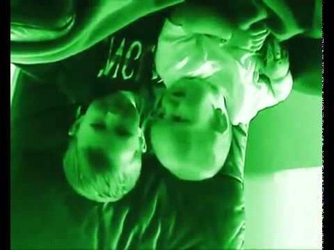
same or similar soundtrack. For example, Figure 1 (a) and The second task is to detect visually similar videos. Giv-
(b) are near duplicates of the song Rolling in the Deep where en a video, we first extract key frames by a shot boundary
(a) is the official video, and (b) is the same song with lyrics. detection algorithm [16] based on the color histogram differ-
Therefore acoustic near duplicate detection is performed for ence between consecutive frames. The frame in the middle
videos whose category is music (in its metadata), and visual of shot is used to represent the shot. SIFT [9] is extracted
near duplicate detection is applied on the rest of the videos. using Harris-Laplace key point detector from the detected
key frames. Following [16], we cluster the SIFT descriptors
into 4,096 clusters using k-means, and quantize them into a
standard bag-of-feature representation. Then, the video is
represented by the averaged bag-of-features of all key frames.
To query a video’s near duplication, we calculate the inter-
section similarity between the given video and the candidate
(a) ID: rYEDA3JcQqw (b) ID:mBRUkdQa6Is videos, and return the top k (k=20) most similar videos as
the detected near duplicate videos.
The above methods are applied to the videos in our dataset.
To evaluate the performance we manually inspect the detec-
tion results of 50 viral videos and 38 music videos. 398
visual near duplicate videos and 1296 acoustical duplicate
videos are detected, i.e. on average 7.96 and 34.1 per video.
(c) ID: OBlgSz8sSM (d) ID: Y13oB-IhE7I Generally, the precision@10 is above 0.9.
Figure 1: Visual and acoustic near duplicate videos.
(a) and (b) are the acoustic near duplicates of the 3. STATISTICAL CHARACTERISTICS
video Rolling in the Deep. (c) and (d) are the visual Table 3 summarizes the statistical characteristics of viral
near duplicates of Charlie Bit my Finger. videos in our dataset. The results are consistent with ex-
isting observations, including the observations on Google’s
The first task is to detect acoustically similar videos i.e. dataset, suggesting the dataset is less biased. For exam-
videos sharing similar soundtracks. Specifically, the Dy- ple, generally, viral videos are less popular than quality
namic Time Warping (DTW) algorithm [6, 12] is adopted videos [2]. They have short titles, durations and lifespan-
to measure acoustic distance between music videos. DTW s [14, 17, 2, 3]. In the rest of the section, we highlight some
was originally proposed for template-based speech recog- interesting characteristics that were revealed in our study.
nition [12] and has been widely used in speech utterance Observation 1: The correlation between the #inlinks re-
matching and spoken term detection [6]. The audio track of turned by Google and #views is a proxy to the socialness.
each music video is represented as a set of 13-dimensional The socialness is a metric to measure the level of dissemina-
MFCC vectors, with a frame length of 25 milliseconds. To tion on social media. Broxton et al. define it as a fraction
reduce potential mismatch due to recording conditions and between the views coming from social sources such as Face-
environments, mean and variance normalization of feature book and non-social sources such as search engines [2]. They
vectors is performed on the whole audio file. The near du- found that viral videos tend to have the higher socialness
plicate detection consists of two steps. First, the DTW dis- compared with other types of videos. Although the observa-
tance for each pair of the given video and its near duplicate tion is interesting, it is impossible to obtain the information
video candidates is computed and normalized by the length on how the user came to watch a video outside Google. We
in each near duplicate group which consists of videos with
Table 4: Evolution of viral videos. essentially the same content. Specifically, two lists can be
Statistics 2010 2011 2012
Days-to-peak Median 24 14 9 obtained within a group; one is the list of metadata e.g. the
Lifespan Median 8 6 3 upload time for each video, the other contains the total views
for each video; PCC is calculated between the two lists.
Figure 2 illustrates the macro-PCC across all near dupli-
cate groups. As we see, the correlation of the upload time
found a publicly available metric that measures the corre-
is not as high as one expects. The factor with the strongest
lation between the #inlinks returned by Google (see social
correlation is the uploader per-video-views, which is the av-
data in Section 2.1) and #views. The correlation reflect-
erage views of all videos uploaded by the uploader, prior to
s the dependency between the social views and the total
the viral video. The result shows that the popularity of the
views. As listed in Table 3, Pearson Correlation Coefficient
uploader is a more important factor in disseminating viral
(PCC) of viral videos is approximately the twice of the oth-
content. The most viewed video in a near duplicate group
ers indicating that the correlation can reasonably estimate
is not necessarily the first uploaded video. In fact, the most
the socialness.
viewed video is, on average, the 2nd to 3rd uploaded video
Observation 2: The days-to-peak and the lifespan of viral
in the group. This phenomenon is more evident for mu-
videos decrease over time. The days-to-peak is the number
sic videos where the official music video usually receives the
of days before reaching the peak view since uploaded. The
most views irrespective of its upload time.
lifespan refers to the number of consecutive days maintain-
ing certain views, which is set to 30% of the peak views in 0.7
our analysis. The medians of both metrics are presented in
Average Pearson Correlation Coefficient
0.6
Table 3. As found in [2], viral videos tend to have both a 0.5
Viral Video
shorter lifespan and shorter days-to-peak. We found that 0.4
Quality Video
these statistics are not static but evolve over time. Table 4 0.3
lists the evolution of the metrics from 2010 to 2012. In 2012, 0.2
on average, it only took 9 days to reach the peak views in 0.1
contrast to 24 days in 2010. The decreasing days-to-peak 0
Uploader per−video views Upload time Title length Average rate
suggests social media has been becoming more efficient in
disseminating viral content. The decrease in the lifespan, Figure 2: The macro Pearson Correlation Coeffi-
on the other hand, perhaps stems from the increasing num- cient between the numeric metadata and the view
ber of interesting videos available on social media. count in near duplicate groups.
Observation 3: Significant correlation can be observed in
the metadata of viral videos. Figure 3 plots the PCC ma-
trix, with each entry indicating the correlation between the
total_upload_views
subscriber_count
corresponding two variables. The magnitude of the correla-
profile_views
num_dislikes
video_views
num_raters
tion is represented by the slope of the ellipse, and the color
num_likes
avg_rate
duration
indicates the correlation type: blue for positive and orange
for negative correlations. Two coefficient clusters can be i- upload_count
dentified. The first one is about users, including the user avg_rate
profile views, the subscriber count and the user’s total up- duration
profile_views
load views. The second one is about videos, including the subscriber_count
number of dislikes, raters and likes. The observation about total_upload_views
these correlations is important as it will influence the choice num_dislikes
of viral videos detection models. Due to the high correlation, num_raters
num_likes
a model explicitly considering the feature correlation, such
as the Bayesian Network [10], may lead to a superior per-
formance. The experimental result in Table 5 substantiates Figure 3: The correlation coefficient matrix in viral
this argument. videos’ metadata. Each entry indicates the correla-
tion between the corresponding two variables. The
Observation 4: The popularity of the uploader is a factor magnitude of the correlation is represented by the
that affects the popularity of the viral video which seems to slope of the ellipse. The color indicates the correla-
be more important than the upload time. It is an interest- tion type: blue for positive and orange for negative
ing phenomenon that some particular videos in a near du- correlations.
plicate group receive significantly higher views than others,
considering that these videos share essentially the same con-
tent. For example, the most popular Gangnam style video
receives 95% of the total views in its near duplicate group 4. FORECASTING THE PEAK DAY
of 28 videos. As the near duplicate videos are uploaded at Based on the observations discussed in Section 3, we in-
different time, the one uploaded earlier has better chance to troduce a novel method to forecast the peak day of viral
become viral. Borghol et al. found background videos have videos. The peak day refers to the date on which a video
this property and coined it as the first mover advantage [1]. reaches its highest views. The ground truth peak day is
We found that for viral videos, though the advantage still known because the daily view count of a video can be ob-
holds, the popularity of the uploader plays a more substan- tained in its insight data. Our method takes a video as
tial role. In order to measure the importance, we calculate input, and outputs the estimated number of days left before
PCC between the numeric metadata and the total views the viral video reaches its peak views. The proposed method
is novel in that it first incorporates the metadata in the peak                       Maximization (EM), only utilizes the view count informa-
day prediction.                                                                       tion. According to Observation 2 and 4, however, ignoring
   According to [2], viral videos usually experience sudden                           the metadata leads to a suboptimal solution. For example,
burstiness in their views. We model the burstiness by a                               according to Observation 2, the lifespan cannot be accurate-
modified HMM which has a single hibernating state h and a                             ly estimated without knowing the upload time. Therefore
series of active states a1 , ..., an . h depicts the state before en-                 we regard P (θ|qt ) as a prior, and estimate it using a classi-
tering or after leaving the burstiness in the view pattern, and                       fier trained on the features available at the current state qt .
the active states model the situation within the burstiness.                          The features are divided into the following groups:
For example, the state sequence h, h, h, a1 , a2 , h describes a                         Bag-of-Words (BoW): Bag-of-words of the video’s title
video that hibernates for the first three days and peaks on                           and text description.
the fifth day. Since the task is to predict the peak day, we                             Time-invariant Metadata: The category, duration, up-
are more interested in the states prior to or at the peak day                         load time, title length, description length and uploader.
than the states after it.                                                                Time-variant Metadata: The accumulated view count,
   A state transits either to the hibernating state or the next                       likes, dislikes and comments up to the current time.
active state, as illustrated in Figure 4. The hibernating state                          The BoW and the time-invariant metadata are time in-
and the last active state (an ) have a self-loop. The symbol                          variant features because their classification values are inde-
emitted by the state is the daily view count which is uni-                            pendent of the state qt . The accuracy of the above features
formly quantized into a set of discrete levels. In other words,                       will be discussed in Section 5.3. Note that we cannot use
the emission probability of each state is a distribution of the                       the features that contain any information after the peak day,
view count levels. The hibernating state models the insignif-                         e.g. #raters, #inlinks and the average rate.
icant number of views outside the burstiness, and thus, the
probability of emitting higher views at the hibernating sta-                                                    0.07                        True Distribution
                                                                                                                                            Gaussian
te should be less than that at an active state. Following                                                       0.06                        Exponential
                                                                                                                                            Cubic Polynomial
the standard notation, let qt denote the state at time t and                                                    0.05

                                                                                                  Probability
                                                                                                                0.04
P (qt+1 |qt ) denote the transition probability from time t to                                                  0.03
t + 1. The emission probability is represented by P (ot |qt )                                                   0.02

where ot is a variable of the emitted symbol, i.e. the view                                                     0.01

count at time t. We assume that the starting state is the                                                         0

hibernating state.                                                                                                     10    20    30     40     50
                                                                                                                            The number of days to peak
                                                                                                                                                       60       70

                                                                                      Figure 5: The distribution of the number of days to
                                                                                      peak (after entering in active states) in our dataset.
                      h             a            a          ...         a           The best fitting of three curves are plotted, namely
                                                                                      Gaussian, Exponential and Cubic Polynomial.
                                            µ
                                                                                         The second modification regards the transition probabili-
                                                                                      ty. The MLE approach estimates the transition probability
                low       high     low   high   low   high         low   high         from state ai to ai+1 as the fraction between the number
                             view count level distribution                            of transitions from ai to ai+1 , and the number of transi-
                                                                                      tions from state ai . However, due to the short lifespan of
Figure 4: The proposed model. θ is a variable on the                                  viral videos in Observation 2, the number of observation-
video type and the emitted symbols are the quan-                                      s decreases sharply as the active state ID becomes larger.
tized view counts.                                                                    For example, our dataset has hundreds of observations for
                                                                                      a1 whereas only less than 10 observations for a12 . A poten-
  Compared with a plain HMM, the proposed model incor-                                tial problem is that the insufficient number of observations
porates two modifications to improve the accuracy. First, it                          may fail to estimate accurate transition probabilities for the
introduces a variable named θ to describe the video type so                           active state with a larger ID. To solve this problem, we s-
that the emission probability can be jointly determined by                            mooth the transition probability by Gaussian distribution.
the current state and the video type. Formally, the emitted                           Empirically, we found the days-to-peak of viral videos (af-
view count is written as:                                                             ter entering the active state) follows the discrete Gaussian
                                 ot = P (θ|qt ) × ôt                           (1)   distribution N (µ, δ 2 ). This assumption may not be optimal
                                                                                      but reasonably captures the distribution (see Figure 5).
where P (θ|qt ) describes the probability of being a viral video                         The transition probability is then calculated from:
at the state qt . ôt is the observed view count at time t, and ot
is the estimated view count given the video is a viral video.                                                                                    X
                                                                                                                                                 i

Since our task is to predict the peak day for viral videos,                                  P (qt+1 = ai+1 |qt = ai ) = 1 −                           αN (k; µ, δ 2 )   (2)
                                                                                                                                                 k=1
P (ot |qt ) is designed to emphasize the views of viral videos.
Given a known ot , P (ot |qt ) can be easily estimated using s-                       where α is a parameter and the second term of the right-
tandard Maximum Likelihood Estimation (MLE) [13]. Note                                hand side is the accumulated probability. Eq. (2) indicates
that the variable θ is incorporated to discount the view coun-                        that the probability transiting to ai+1 equals the probability
t, rather than conventionally incorporated as a latent vari-                          not peaking before the state ai . Only three parameters i.e.
able in the graphic model, because we found that this strat-                          α, µ and δ need to be estimated and can be derived by
egy works reasonably well in practice. Besides, estimating                            regression on the observations in the training set.
latent variable in the graphic model, usually by Expectation                            Since the ground truth daily views of a video can be ac-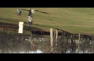
cessed in its insight data, the hidden state can be auto-                    as to peak at a future state, and according to Eq. (6), it is
matically assigned, and the proposed model can be trained                    less likely to happen. Therefore when qt is an active sta-
on viral videos by the standard Baum-Welch algorithm [13].                   te in {ai |1 ≤ i < n}, Eq. (4) selects the most likely state
Once the model is trained, the next task switches to the peak                sequence from all possible sequences. The following toy ex-
day prediction. Given an observation sequence o1 , ..., ot ,                 ample shows how to calculate the peak state.
Viterbi algorithm can be applied to estimate the most like-
                                                                                Example 1. Suppose the symbols: “low”, “med” and “high”
ly sequence of corresponding hidden states up to the cur-
                                                                             represent the quantized view count levels using Eq.(1) and
rent time. A video is estimated to peak at state qt+k , if                   the trained HMM is in Figure 6. We have the following ob-
qt+k 6= h ∧ qt+k+1 = h, which is the last state before tran-
siting back to the hibernating state. Physically, the peak
                                                                                                                      0.2                0.4           0.6
state corresponds to the day with the highest views. As
                                                                                                       0.10                 0.8                0.6
mentioned, we are more interested in modeling the states
before the peak day. We do not explicitly model the states                               0.90                                                   0.4
after the peak day because they are less important for the
                                                                                         high   0.05      high        0.50        high     0.60       high   0.80
peak day prediction. More formally, suppose at the current                               med    0.05      med         0.15        med      0.20       med    0.15
time t, the state estimated by Viterbi algorithm is qt , the                             low    0.90      low         0.35         low     0.20       low    0.05
prediction task is to find the peak state qpeak in the most
likely sequence starting with qt , i.e.                                         Figure 6: A toy example of the trained model.
              qpeak = arg max P (qt , qt+1 , ..., qt+k , h),        (3)
                           k                                                 servation sequences:
                                                                                    ID     observation sequence                                  state sequence
where k is the number of days left before the peak. To
                                                                                     1     low, low, med                                         h, h, h
calculate the joint probability we rewrite it as                                     2     low, low, high                                        h, h, a1
                                                                                     3     low, low, high, med, high,                            h, h, a1 , a2 , a3
           arg maxk P (h|ai+k ) i+k−1
                              Q
                                j=i   P (aj+1 |aj )    qt = ai (1 ≤ i < n)
qpeak =
           qt                                          otherwise             Feeding the observation sequences to Viterbi algorithm, we
                                                                      (4)    get the corresponding most likely state sequences up to the
where i + k ≤ n, and n is the total number of active states6 .               current time. For the first case (ID=1) and last case (ID=3),
Eq. (4) is more computationally efficient than Eq. (3), and                  the current state is h and a3 , according to Eq. (4), the peak
can be solved by enumerating all possible k < n. It indicates                state is the current state i.e. the video will not peak in future.
that when the current state is one of the active states except                  For the second case, we calculate the probability of all pos-
                                                                             sible sequence starting from a1 :
an , the peak state is in the most likely sequence. Otherwise,
                                                                                P (h|a1 ) = 0.2,
when the current state is either the hibernating state or the                   P (h|a2 )P (a2 |a1 ) = 0.4 × 0.8 = 0.32,
last active state an , the peak state is the current state. To                  P (h|a3 )P (a3 |a2 )P (a2 |a1 ) = 0.6 × 0.6 × 0.8 = 0.28.
prove when qt = an , qpeak = qt = an , we have:                                 Since a1 a2 h is the most likely sequence, the peak state
                                                                             qpeak = a2 and the number of days left to peak is thus 1.
P (qt = an , qt+1 = an , qt+2 = h)
= P (qt = an )P (qt+1 = an |qt = an )P (qt+2 = h|qt+1 = an )                 5. EXPERIMENTS
= P (qt = an )P (qt+1 = an |qt = an )P (qt+1 = h|qt = an )
= P (qt = an , qt+1 = h)P (qt+1 = an |qt = an )                              5.1 Experimental Setup
≤ P (qt = an , qt+1 = h).                                  (5)                  To validate the efficacy of the proposed method on the
                                                                             peak day prediction for viral videos, we conducted experi-
Similarly we can also verify that qt = h then qpeak = h.                     ments on the videos with the insight data in our dataset.
   If the current state is one of the active states other than               Since the daily view count is available in the insight da-
an , according to Eq. (4) at most n − 1 sequences need to be                 ta, the ground truth peak day of a video was set to the
calculated. It is because, as proved in Eq. (5), that when                   date with the largest view count. Following [11], the date
a state is at an , the most likely next state is h. It can                   at which a method makes predictions is called the reference
also be shown that at any time t (t ≥ 1), the probability                    date. Each method can access any information before and
of re-entering the active state is less than the probability of              after the reference date in the training set. However, it on-
transiting back to the hibernating state. Formally we have:                  ly allow to use information before the reference date in the
                           X                                                 test set in order to forecast the peak day in future. Since
     P (qt , qt+1 = h) =          P (qt , qt+1 = h, ..., qt+m )              the task is to forecast the peak day for viral videos, an ideal
                           qt ,...,qt+m                                      system should only report the peak day for viral videos and
     > P (qt , qt+1 = h, qt+2 = a1 ),                               (6)      remain silence for non-viral videos. The viral and non-viral
                                                                             videos were equally divided into a training and a test set. A
where m (m ≥ 2) is a parameter indicating the length of                      commonly used metric AP (Average Precision) was used to
the state sequence. The left-hand side of Eq. (6) is the                     evaluate the precision of estimated peak days, which is im-
probability of peaking at the state qt . The right-hand side                 mune to the threshold in prediction methods. We compared
indicates the probability of re-entering the active states so                the proposed method with the following baseline methods:
6                                                                               Plain HMM [13]: Plain HMM without the variable θ,
  The short lifespan observation in Section 3 indicates that
P (h|h) > P (h|a) that is a video stays in the hibernating                   but with smoothed transaction probability discussed in Sec-
state for the most of time. Relaxing this condition is trivial.              tion 4.
Enumerating all the state sequences starting from h using                       S-H Model [15]: S-H (Szabo-Huberman) Model is a
the same method for active states in Eq. (4).                                video popularity prediction model. The model assumes that
0.8
there exists a strong linear correlation between a video’s ac-                                                 Our Method

cumulated views and views in future. Following the notation                                             0.7    Plain HMM
                                                                                                               SVM Regression
in [11], suppose N (tr ) represents the accumulated views up                                            0.6
                                                                                                               S−H Model

                                                                                    Average Precision
                                                                                                               ML Model
to the reference date tr . tt (tt > tr ) denotes the views in fu-                                       0.5
ture. We have ln N (tt ) = ln r(tr , tt )N (tr ) + ξ, where r(tr , tt )
is a parameter and ξ is the Gaussian noise term. Given a                                                0.4

reference date, we trained a regression model to estimate the                                           0.3

weight r(tr , tt ) in the training data.                                                                0.2
   ML Model [11]: S-H model can be regarded as a re-
                                                                                                        0.1
gression model with a single explanatory variable, i.e. the                                              −10   −9    −8         −7    −6    −5     −4
                                                                                                                                 Days Since Peak View
                                                                                                                                                        −3   −2   −1

accumulated view count. Multivariate Linear (ML) Mod-
el considers several explanatory variables, each of which                 Figure 7: Performance comparison with baseline
is a delta view sampled before the reference date. For-                   methods in terms of AP. The x-axis represents the
mally, the prediction is based on the regression function                 date, at which the method makes predictions, rela-
N (tt ) = Θ(tr ,tt ) Xtr , where Xtr is the feature vector of delta       tive to the true peak day.
views, and Θ is a vector of parameters to estimate.
   SVM Regression: SVM regression further extends the
S-H model to incorporate the metadata (both time invariant                mance suggesting the linear correlation assumption [15] is
and variant) into the explanatory variables. It also intro-               violated in viral videos. According to Observation 3 in Sec-
duces a l2 regularization term to avoid overfitting.                      tion 4, viral videos usually experience sudden burstiness in
   The baseline methods were selected based on two con-                   their views, and obviously the view count before entering the
siderations: (1) the methods cover both the well known [13]               burstiness does not correlate to the views in the burstiness.
and the state-of-the-art methods [15, 11]; (2) the comparison             SVM Regression also adopts the same assumption. But be-
between them helps to isolate the contribution of different               cause it uses the metadata, it is slightly better than S-H and
components. For example, the contribution of the variable                 ML model.
θ can be demonstrated by comparing the proposed method
with the plain HMM. Likewise, the contribution of addi-                   5.3 Accuracy of Prior Estimation
tional features can be shown by comparing SVM Regression
                                                                              To study the importance of each feature discussed in Sec-
with S-H Model. The parameters in the proposed method
                                                                          tion 4, we compared the accuracy of prior estimation with
were selected in terms of the cross-validation performance
                                                                          different types of features and classifiers. Since prior esti-
on the training set. For example, the number of active sta-
                                                                          mation can be regarded as a classification problem, F1 was
tes was set to 11; the estimated parameters in Eq. (2) were
                                                                          adopted to evaluate the accuracy. Table 5 lists the compari-
α = 0.0529 µ = 12.79 and δ = 9.665; the views were uni-
                                                                          son results. Generally, time-invariant metadata turns out to
formly quantized into five levels according to Eq. (1). By
                                                                          be the single best feature. The result suggests that the char-
default, the prior in Eq. (1) was estimated using the late
                                                                          acteristics in Table 3, including the duration, title length, are
fusion of all three types of features discussed in Section 4.
                                                                          effective in distinguishing viral videos. While the reference
The words in the BoW features were stemmed using Porter
                                                                          date is approaching the true peak day, more information is
Stemmer after removing the stop words, and only symbols
                                                                          available, resulting in the increased accuracy of the time-
and English words were included in the vocabulary.
                                                                          variant metadata. On the other hand, the BoW features
                                                                          and the time-invariant metadata, which are independent of
5.2 Comparison with Baseline Methods                                      the reference date, remain unchanged. Regarding the classi-
   Figure 7 compares the performance of the baseline meth-                fier, the linear SVM classifier outperforms others with BoW
ods, where the x-axis denotes how many days the reference                 features. Bayesian Network achieves the best performance
date is prior to the true peak day. Generally, all methods                on both time-variant and time-invariant metadata. The re-
become more accurate while the reference date approaching                 sult substantiates the analysis in Section 4 that a classifier
the true peak day. The proposed method outperforms al-                    modeling correlations in metadata leads to a better perfor-
l baseline methods, and according to the paired t-test, the               mance. Random Forest is the most robust classifier across
improvement is significant at the P-value 0.001 level. This               features. The SVM classifier gets worse performance on the
result demonstrates that the proposed method’s efficacy in                metadata features suggesting that the problem is nonlinear
forecasting viral videos. Figure 8 shows examples of the                  separable in the low dimensional feature space.
peak day prediction result.                                                  To study the impact of the accuracy of prior on the peak
   Compared with a plain HMM, the superior performance                    day prediction, we conducted experiments where the prior
of the proposed method stems from the consideration of the                estimated by each feature was added, one at a time, to the
video type. The introduced variable θ leverages metadata to               proposed method. The experiment was designed to isolate
identify viral videos before the peak day. It can adjust the              the contribution brought by each feature. Figure 9 illus-
emission probability to emphasize the view counts of viral                trates the comparison result. Generally, as we see, the prior
videos. In contrast, the plain HMM ignores this information               plays an important role in the peak day prediction. A bad
and often confuses viral and quality videos. This argumen-                prior, e.g. Description BoW, may result in a worse model
t can also be verified by comparing S-H model and SVM                     than the plain HMM. The best single feature is the time-
regression, where their difference lies in the usage of meta-             invariant metadata, which seems to be consistent to its high
data in prior estimation. Therefore, the results substantiate             F1 discussed above. The best prior is the late fusion of all
our argument that considering metadata is beneficial in this              features suggesting the proposed features are of complemen-
task. S-H model and ML model have the poorest perfor-                     tary information.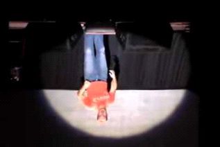
Viral Videos
Golden Eagle Evolution of The Sneezing Friday - HOW TO PLAY:
Reference Date Snatches Kid Dance Baby Panda Rebecca Black P!nk
7 days before the true peak day peak in 7 days peak in 9 days peak in 6 days peak in 9 days Not a viral video
3 days before the true peak day peak in 3 days peak in 3 days peak in 2 days peak in 6 days Not a viral video
It will peak It will peak It will peak
1 day before the true peak day peak in 2 days
tomorrow. tomorrow. tomorrow. Not a viral video
Figure 8: Examples of viral videos’ peak day prediction, on different days before the ground truth peak day.
leagues, editors from Time Magazine, and YouTube for an-
Table 5: Comparison of the prior estimation with notating viral videos. The authors would like to express
different features and classifiers in terms of F1 . NB
for Naive Bayes; BN for Bayesian Network; RF for gratitude to William Cohen, Bhavana Dalvi and Aasish Pap-
Random Forest. pu for the useful comments and remarks.
Time Unrelated NB SVM BN RF
Title BoW 0.36 0.40 0.06 0.19
Description BoW 0.28 0.29 0.02 0.04 8. REFERENCES
Time-invariant metadata 0.37 0.16 0.54 0.45 [1] Y. Borghol, S. Ardon, N. Carlsson, D. Eager, and A. Mahanti.
Time-variant Metadata NB SVM BN RF The untold story of the clones: content-agnostic factors that
impact youtube video popularity. In SIGKDD, pages
-10 days since the true peak day 0.05 0.03 0.26 0.18 1186–1194, 2012.
-7 days since the true peak day 0.05 0.03 0.41 0.34
-3 days since the true peak day 0.05 0.05 0.52 0.36 [2] T. Broxton, Y. Interian, J. Vaver, and M. Wattenhofer.
-1 days since the true peak day 0.05 0.05 0.53 0.45 Catching a viral video. Journal of Intelligent Information
On the true peak day 0.05 0.05 0.54 0.50 Systems, 40(2):241–259, 2013.
[3] J. Burgess. All your chocolate rain are belong to us. Video
Vortex Reader: Responses to YouTube, pages 101–109, 2008.
1 [4] R. Crane, D. Sornette, et al. Viral, quality, and junk videos on
Late Fusion youtube: Separating content from noise in an information-rich
0.9 Plain HMM environment. In AAAI symposium on Social Information
Time−invariant meta−data
0.8
Title BoW
Processing, 2008.
[5] F. Figueiredo, F. Benevenuto, and J. M. Almeida. The tube
Average Precision
0.7
Description Bow
Time−variant meta−data over time: characterizing popularity growth of youtube videos.
0.6 In WSDM, pages 745–754, 2011.
[6] T. Hazen, W. Shen, and C. White. Query-by-example spoken
0.5
term detection using phonetic posteriorgram templates. In
0.4 ASRU, pages 421–426, 2009.
[7] L. Jiang, Z. Wu, Q. Feng, J. Liu, and Q. Zheng. Efficient deep
0.3 web crawling using reinforcement learning. In PAKDD, pages
0.2
428–439, 2010.
−10 −9 −8 −7 −6 −5 −4 −3 −2 −1 [8] L. Jiang, Z. Wu, Q. Zheng, and J. Liu. Learning deep web
Days Since Peak View crawling with diverse features. In Web Intelligence, pages
572–575, 2009.
[9] D. Lowe. Distinctive image features from scale-invariant
Figure 9: The influence of the different priors on the keypoints. IJCV, 60(2):91–110, 2004.
prediction precision. [10] F. Pernkopf. Bayesian network classifiers versus selective k-nn
classifier. Pattern Recognition, 38(1):1–10, 2005.
[11] H. Pinto, J. M. Almeida, and M. A. Gonçalves. Using early
view patterns to predict the popularity of youtube videos. In
6. CONCLUSIONS AND FUTURE WORK WSDM, pages 365–374, 2013.
[12] L. Rabiner, A. Rosenberg, and S. Levinson. Considerations in
We established by far the largest open dataset of viral dynamic time warping algorithms for discrete word recognition.
videos to date. Having verified existing observations, we Acoustics, Speech and Signal Processing, IEEE Transactions
discovered some interesting characteristics of viral videos, on, 26(6):575–582, 1978.
[13] L. R. Rabiner. A tutorial on hidden markov models and
including the metric of measuring socialness, the evolution selected applications in speech recognition. Proceedings of the
of the lifespan, and the correlation residing in the metadata. IEEE, 77(2):257–286, 1989.
[14] G. Rocket. Emerging trends in viral video and the implications
By studying near duplicate videos, we found that the popu- for advertising. http://www.slideshare.net/GeniusRocket/viral-
larity of the uploader is a more important factor for a video video-research-presentation.
go viral than the upload time. Inspired by our analysis, [15] G. Szabo and B. Huberman. Predicting the popularity of online
content. Communications of the ACM, 53(8):80–88, 2010.
we introduced a novel approach to forecast the viral video’s [16] W. Tong, Y. Yang, L. Jiang, S.-I. Yu, Z. Lan, Z. Ma, W. Sze,
peak day in future. The proposed method is the first at- E. Younessian, and A. G. Hauptmann. E-lamp: integration of
innovative ideas for multimedia event detection. Machine
tempt to incorporate metadata in the peak day prediction. Vision and Applications, pages 1–11, 2013.
The empirical results demonstrate that the proposed method [17] T. West. Going viral: Factors that lead videos to become
outperforms the state-of-the-art methods with statistically internet phenomena. Elon Journal of Undergraduate Research,
pages 76–84, 2011.
significant difference. We have only used the endogenous [18] X. Wu, A. Hauptmann, and C. Ngo. Practical elimination of
features available on YouTube. In future, we plan to exploit near-duplicates from web video search. In ACM Multimedia,
pages 218–227, 2007.
both endogenous and exogenous features such as the number [19] L. Xie, A. Natsev, J. R. Kender, M. Hill, and J. R. Smith.
of tweet mentions to forecast the peak day of viral videos. Visual memes in social media. In ACM Multimedia, pages
53–62, 2011.
[20] R. Zhou, S. Khemmarat, and L. Gao. The impact of youtube
7. ACKNOWLEDGMENTS recommendation system on video views. In SIGCOMM
Conference on Internet Measurement, pages 404–410, 2010.
The authors are grateful to William Johnson and his col-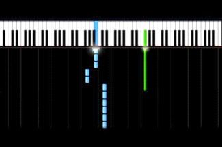
You can also read