EON: software for long time simulations of atomic scale systems
←
→
Page content transcription
If your browser does not render page correctly, please read the page content below
Modelling and Simulation in Materials Science and Engineering

Modelling Simul. Mater. Sci. Eng. 22 (2014) 055002 (16pp)                      doi:10.1088/0965-0393/22/5/055002

EON: software for long time simulations of
atomic scale systems

                  Samuel T Chill1 , Matthew Welborn1 , Rye Terrell1 ,
                  Liang Zhang1 , Jean-Claude Berthet2 , Andreas Pedersen2 ,
                  Hannes Jónsson2 and Graeme Henkelman1
                  1
                    Department of Chemistry and the Institute for Computational Engineering and
                  Sciences, The University of Texas at Austin, Austin, TX 78712-0165, USA
                  2
                    Faculty of Physical Sciences and Science Institute, University of Iceland, 107
                  Reykjavı́k, Iceland

                  E-mail: hj@hi.is and henkelman@cm.utexas.edu

                  Received 23 November 2013, revised 1 March 2014
                  Accepted for publication 8 April 2014
                  Published 9 May 2014

                  Abstract
                  The EON software is designed for simulations of the state-to-state evolution of
                  atomic scale systems over timescales greatly exceeding that of direct classical
                  dynamics. States are defined as collections of atomic configurations from which
                  a minimization of the potential energy gives the same inherent structure. The
                  time evolution is assumed to be governed by rare events, where transitions
                  between states are uncorrelated and infrequent compared with the timescale
                  of atomic vibrations. Several methods for calculating the state-to-state
                  evolution have been implemented in EON, including parallel replica dynamics,
                  hyperdynamics and adaptive kinetic Monte Carlo. Global optimization
                  methods, including simulated annealing, basin hopping and minima hopping
                  are also implemented. The software has a client/server architecture where
                  the computationally intensive evaluations of the interatomic interactions are
                  calculated on the client-side and the state-to-state evolution is managed by the
                  server. The client supports optimization for different computer architectures
                  to maximize computational efficiency. The server is written in Python so that
                  developers have access to the high-level functionality without delving into the
                  computationally intensive components. Communication between the server
                  and clients is abstracted so that calculations can be deployed on a single
                  machine, clusters using a queuing system, large parallel computers using a
                  message passing interface, or within a distributed computing environment. A
                  generic interface to the evaluation of the interatomic interactions is defined so
                  that empirical potentials, such as in LAMMPS, and density functional theory as
                  implemented in VASP and GPAW can be used interchangeably. Examples are
                  given to demonstrate the range of systems that can be modeled, including

0965-0393/14/055002+16$33.00   © 2014 IOP Publishing Ltd   Printed in the UK                                    1
Modelling Simul. Mater. Sci. Eng. 22 (2014) 055002 S T Chill et al
surface diffusion and island ripening of adsorbed atoms on metal surfaces,
molecular diffusion on the surface of ice and global structural optimization of
nanoparticles.
Keywords: rare event dynamics, transition state finding, saddle points, adaptive
kinetic Monte Carlo, accelerated molecular dynamics
(Some figures may appear in colour only in the online journal)
1. Introduction
Long timescale simulations of atomic systems pose a particular challenge in computational
chemistry. A straightforward integration of the equations of motion typically requires too
many integration steps to reach the timescale of interesting events. Since atomic vibrations
occur on the femtosecond timescale, roughly 1015 time steps are required to directly model
one second of molecular dynamics (MD).
EON is a software package for performing accelerated dynamics simulations of diffusion
in solids and reactions at surfaces. There are a number of established methods for calculating
the long timescale properties of chemical and material systems and a primary goal of EON is to
provide these methods in a single program so that they can be directly compared, the strengths
of different methods exploited, and where advantageous, combined into hybrid methods.
The methods implemented in EON share an underlying concept. They each assume that
the system has stable states that correspond to minima on the potential energy surface (PES).
The term ‘stable’ means that the average escape time from a state is significantly greater than
the correlation time of a trajectory within the state. The transitions between states are then
rare events in comparison to the vibrational relaxation timescale within any state.
The computational framework for the methods implemented in EON is illustrated in figure 1.
EON has a client-server architecture in which the server determines the state-to-state evolution
of the system. Clients communicate with the server to receive tasks that involve exploring
the configuration space around the current state. Results are reported back to the server so
that the state-to-state evolution can proceed. For both receiving work and reporting results,
communication is initiated by the client and the simulation data is transmitted in human readable
text files.
The implementation of EON is illustrated in figure 2. The client, written in C++, performs
computationally intensive tasks, while the server, written in Python, handles the bookkeeping
associated with the higher-level algorithms. The client is used for any method that requires
evaluation of the potential energy and force. Client-side methods include local geometry
optimization, saddle point searches, MD trajectories, Monte Carlo sampling and normal mode
analysis. The server implements the high-level methods using the tools provided by the client
including parallel replica dynamics (PRD) [1], hyperdynamics [2] using the bond-boost form
of the bias potential [3], adaptive kinetic Monte Carlo (AKMC) [4], basin hopping (BH) [5]
and minima hopping [6].
The EON architecture has several strengths. First and foremost, the client-server
architecture allows for asynchronous cluster and distributed computing. Second, a single
server can communicate with many different clients through a common interface, meaning
that only part of the code has to be tailored to different platforms, either through compilation
or linking to platform-specific libraries. Finally, the server communicates with the client via
2Modelling Simul. Mater. Sci. Eng. 22 (2014) 055002 S T Chill et al
state to state
state i transitions
state i+1
server
communicator
clients
exploring
state i+1 ...
exploring
state i
Figure 1. Computational framework of EON calculations.
Server Client
Read Start Jobs Load Data Task Communicate Read Input Run Jobs Use Methods Optimize
Config Adaptive KMC Atoms Creation Files Basin Hopping Basin Hopping Conjugate-
Local
Parallel Replica State Prefactor Minimization Gradients
Cluster
Hyperdynamics Super Basin Basin Constrained MD MD Quickmin
Boinc
Basin Hopping State List Single Point Energy NEB FIRE
MPI
Minimization Hessian LBFGS
ARC
Hessian Dimer / Lanczos
NEB
Start Store Data ProcessResults Communicate Write Output MD Potential Evaluation
Files Process Search
Atoms Adaptive KMC
Parallel Replica Replica Exchange Lenosky / Tersoff (Si) LAMMPS
State
Basin Hopping Saddle Search Lennard-Jones VASP
Super Basin
TIP4P (water) GPAW
State List
EAM / EMT QSC
Generic MPI EDIP (C)
Figure 2. The EON server interacts with EON clients through communicators, providing
them with independent tasks (e.g. saddle searches). The results are communicated back
to the server where they are processed by higher-level algorithms (e.g. adaptive kinetic
Monte Carlo). The various acronyms are defined in the text.
text files so that a user can directly access the client’s functionality without having to use the
server.
2. Code structure
2.1. Server
The EON server has several roles: managing the execution of client jobs, processing the results
of client calculations and transitioning between states of the system. Typically the server is
run many times over the course of a calculation. Upon each invocation, the server processes
the results of completed jobs, performs actions depending on the results that were received
and creates new jobs, in that order. EON will typically exit at this point. The one exception is
when EON is run with the message passing interface (MPI) communicator, in which case the
server will continue to run in a loop waiting for new results to process.
The EON server coordinates a set of independent tasks, which are executed in parallel
by the clients. The primary mechanism of communication between client and server is via
human-readable text files. The server creates the input files for each client calculation and
processes the output files that the clients write. The results of the individual client calculations
influence subsequent jobs; it is only through the server that the clients interact.
3Modelling Simul. Mater. Sci. Eng. 22 (2014) 055002 S T Chill et al
In a distributed computing environment, clients cannot be trusted to complete all of the
work that they are given. In a heterogeneous computing environment, clients will typically
leave and return to the network over the course of an EON simulation. Due to this constraint,
server-client communication is stateless; no one client is relied upon to complete any given
job. Instead, enough work is created to keep all clients busy and the results are processed upon
their completion. The server never waits for a particular client to finish a calculation.
The independence of the client jobs allows for flexibility in how the clients are executed.
EON supports parallel calculations in a variety of contexts: on a single computer, on clusters
using a queuing system, large parallel computers using MPI and in a distributed computing
environment. These contexts are explained more fully in section 2.4.
The server also manages the state-to-state evolution in the system. For example, in the
AKMC method, the server uses the kinetic Monte Carlo (KMC) algorithm to move between
states until an unexplored state is reached. At this point, client calculations are required to
determine the mechanisms and rates of escape. In PRD, the server waits for clients to run
dynamics within a state and report transitions a new state. The server then updates the current
state of the system and repeats the process.
2.2. Client
While the server is written in Python, the client is written in C++. An advantage of using a
complied language for the client is that a self-contained executable is most easily used within
a distributed computing platform [7]. A Python client would require the distribution of the
Python runtime environment along with our code. Another reason for using C++ is that the
client does most of the computational work, and it is not uncommon for Python to be 100 times
slower than lower level languages [8].
EON provides a number of reusable software components. For example, the numerical
optimization routines operate on general objective functions. This allows the same optimization
code to be applied to a variety of problems, including local minimization, saddles searches
and nudged elastic band calculations. EON implements a number of first and second order
optimization algorithms including quick-min (QM) [9], fast inertial relaxation engine (FIRE)
[10], conjugate gradients (CG) [11] and limited-memory Broyden–Fletcher–Goldfarb–Shanno
(L-BFGS) [12].
2.3. Potentials
EON makes use of a variety of different atomic interaction potentials, some of which are
implemented within our code while others are accessed either by linking to a library or calling an
external program. Specifically, EON works with the Large-scale Atomic/Molecular Massively
Parallel Simulator (LAMMPS) [13], the Vienna Ab-initio Simulation Package (VASP) [14] and the
Grid-based Projector-Augmented Wave (GPAW) [15] code.
The potentials that are included with EON are an embedded atom method (EAM) potential
[16] with parameters for Al [17], quantum Sutton-Chen with parameters for FCC metals,
effective medium theory from the ASAP package [18], pair potentials of the Lennard-Jones
and Morse forms, Lenosky [19] and Tersoff [20] potentials for Si, the environment dependent
interactive potential (EDIP) for carbon [21] and the TIP4P water model [22].
EON can use potentials from LAMMPS by linking EON to the LAMMPS library. The LAMMPS
interface in EON issues commands to initialize the simulation by specifying the periodic
boundary conditions and atom types. For each force call, EON updates the positions of the
atoms in LAMMPS and calls the application programming interface (API) to update the energy
4Modelling Simul. Mater. Sci. Eng. 22 (2014) 055002 S T Chill et al
and forces. Using the API, as opposed to calling the LAMMPS executable for each force call, keeps
the neighbor list in memory between force calls, and significantly improves the computational
efficiency.
Finally, there is a MPI-based potential interface that communicates with an external MPI
program to calculate the energy and forces. This potential type is implemented as a multiple
program multiple data (MPMD) MPI job where the EON client is launched along with the
external MPI program(s). Having a single executable for the server and clients is especially
useful for running on supercomputers with ab initio codes that do not have a library interface
to be linked with EON. An example of such a program is VASP. We provide a small modification
to VASP to work with EON so that VASP stays in memory between energy evaluations [23]. In our
tests this approach is 60% faster than executing VASP for each force call, reusing the previous
wavefunctions and charge density from disk.
2.4. Communicators
The client-server architecture gives EON flexibility in how the client program is executed. The
details of how the client runs and communicates its results are abstracted. Decoupling the
communication from the rest of the code allows for different parallelization schemes to be
implemented with minimal effort. The different communicators are implemented as classes
that handle how and where the client is executed. The interface to the class is simple, requiring
only the data in the input files for the client. The specific communicator then ensures that the
job is executed and returns the result, when completed, to the server. The class also provides
methods to cancel jobs and retrieve the number of running jobs.
Our generic approach to running the computationally expensive part of our program allows
EON to run in the following modes.
Local: the simplest way to run EON is to run in serial or in parallel on a single computer.
The server launches a user specified number of jobs in parallel and waits for them to complete
before exiting.
Cluster: EON can directly submit jobs to a job queuing system such as Grid Engine, Torque,
or the Portable Batch System (PBS). User supplied scripts enable the EON server to submit
jobs, monitor running jobs and delete jobs.
MPI: with the MPI communicator, the server and clients are bundled together as a single
MPMD MPI executable. The server, instead of exiting after creating client jobs, polls the
clients to determine when new jobs need to be created. When combined with the MPI
potential interface, EON can run many independent density functional theory (DFT) calculations
simultaneously.
BOINC: EON supports distributed computing using the Berkeley Open Infrastructure for
Network Computing (BOINC) [7]. Running a distributed calculation requires a BOINC project
server and an EON client that is linked with the BOINC library. EON is currently run as a BOINC
project with over a thousand computers connected that has achieved a peak performance of
four teraFLOPS. [24]. It is possible to run many independent calculations using the same BOINC
project with EON. The communicator uses a unique identifier to track which BOINC work units
belong to which simulation. In this way, multiple users are able to run their own simulations
within the same BOINC project.
5Modelling Simul. Mater. Sci. Eng. 22 (2014) 055002 S T Chill et al
A consideration when using BOINC for calculations is that the communication time between
client and server should be shorter than the time to complete a client job. For calculations
involving empirical potentials, a single client calculation can be faster than the time to process a
work-unit through the distributed computing system. This condition causes the client computer
to be idle while it waits for additional work. To solve this problem, we have implemented a
mechanism for bundling a set of tasks together to be run as a single client job. Tuning the
number of tasks in the bundle controls the BOINC work unit duration. Bundling a set of small
jobs into work units also reduces the number of files which have to be processed by the server,
an issue that becomes very important when thousands of machines are rapidly reporting their
result to a single server.
ARC: an interface for the Advanced Resource Connector (ARC) middleware enables execution
on resources connected to NORDUGRID [25]. The purpose of the interface is to enable to use of
idle nodes on authorized resources. As only idle resources are to be requested, one initially
registers how many idle nodes each cluster has, which is followed by a submission of the
corresponding number of work units to the NORDUGRID queue on each of the clusters. The ARC
middleware must be installed with the EON server to use this communicator.
3. Methods
3.1. PRD and hyperdynamics
PRD is a method for parallelizing state-to-state MD trajectories [1]. A set of M replicas of the
simulation are initialized to run MD trajectories on separate processors from the same initial
state. Each replica is given its own unique initial random momenta and run with MD for a
short dephasing time to ensure that it is uncorrelated from the other replicas in configuration
space. After dephasing, the simulation clock is started and MD is performed until any replica
has escaped from the initial state. All replicas then report the amount of time that has been
simulated and the transition time is taken to be the cumulative simulation time from the replicas.
Critical to this method is an algorithm to detect transitions between states. In EON, we detect
a transition by periodically minimizing the geometry and comparing to the initial minimized
geometry.
The algorithm, as described, is not suitable for distributed computing because it is not
always possible to promptly report when a replica sees a transition, nor is it possible to query
all the other replicas to determine how much simulation time had been accumulated when the
transition occurred. To work with EON, all communication between replicas must be removed.
This is accomplished in the distributed replica dynamics (DRD) implemented in EON by having
each client run for a fixed length trajectory. The clients do not report back when they detect a
reaction; instead, each replica does the same amount of work as all other clients, on average.
Accordingly, when a client detects a transition it records the transition time and configuration
and then continues to run dynamics for the full time length as if a transition had not occurred.
It then returns the time of the transition and the new product state to the server. The server
adds the transition time to the total simulation clock. Details of the validity and efficiency of
the DRD algorithm will be presented elsewhere [26]. Since DRD is so similar in philosophy
to PRD, we will refer to it hereafter simply as PRD.
As an example of a long timescale simulation modeled with PRD, we have chosen the
formation of a compact Pt heptamer island on Pt(1 1 1) at 250 K using a Morse interatomic
potential. Each PRD client was run for a 20 ps MD trajectory with a time step of 2 fs and a
dephasing time of 1 ps. PRD was also combined with hyperdynamics to increase the accessible
6Modelling Simul. Mater. Sci. Eng. 22 (2014) 055002 S T Chill et al
0s 0s 1 µs 1 µs 0.6 ms 0.7 ms
0 Parallel Replica Dynamics
-1 Hyperdynamics
-2
Energy (eV)
-3
-4
-5
-6
-7
-8
-12 -9 -6 -3
10 10 10 10
Time (s)
Figure 3. Snapshots from PRD and hyperdynamics simulations of seven Pt atoms
randomly deposited on a (1 1 1) surface at 250 K. The final state, which is found using
hyperdynamics on a timescale of minutes, shows the formation of a compact heptamer
island. The atoms on the surface are shaded red.
simulation time. We used the bond-boost form of bias potential [3] setting the magnitude of
the total boost !V max to 0.5 eV, the stretch threshold q to 0.2 and the curvature parameter P1
to 0.95. All other parameters were kept the same as the PRD calculation. The evolution of the
system is shown in figure 3. The initial coalescence of the adatoms occurs on a timescale of
nanoseconds and the formation of the compact island occurs on a timescale of minutes, which
can only be seen in the hyperdynamics simulation.
In the ideal case, PRD is able to reduce the wall-clock time of a MD calculation linearly
with respect to the number of processors used. To demonstrate that our code achieves this
scaling, we measured the speed-up of escaping from the compact Pt heptamer island state.
Each PRD trajectory was run for 100 ps; reactive events were detected by minimizing every
10 ps. Figure 4 shows that the speed-up, in terms of wall-clock time, required to find an escape
time for the compact Pt heptamer island on Pt(1 1 1) increases linearly with the number of
replicas. The slope of the speed-up plot only deviates from unity when the total time simulated
by the replicas in a reporting interval approaches the transition time. When there are M
clients running 100 ps trajectories in parallel, this limit is reached for M ≈ 100 at 500 K and
M ≈ 1000 at 400 K. In principle, the MD time simulated by each replica can be reduced,
although here, 100 ps was chosen so that each calculation would take several minutes, which
is a suitable job length for distributed computing, as discussed in section 2.4.
3.2. Adaptive kinetic Monte Carlo
KMC is a method used to model the state-to-state dynamics of chemical and material systems.
An in-depth introduction and discussion of the history of KMC has been written by Voter [27].
KMC simulations are fundamentally different from MD in that they do not need to evaluate
the potential energy or forces of the system, although in many cases, rates of reaction are
derived from a PES. In KMC, a Markov chain of states is formed with transition probabilities
7Modelling Simul. Mater. Sci. Eng. 22 (2014) 055002 S T Chill et al
1536
768
384
192
96
Speed Up 48
24
12
6
3
400K (1.4 us)
500K (6.3 ns)
1
1 3 6 12 24 48 96 192 384 768 1536
Number of Replicas
Figure 4. Timing data showing good linear speedup for PRD of a Pt heptamer island
on Pt(1 1 1). Deviations from the linear scaling trend start when the number of replicas
times the simulation time for each replica approaches the timescale of the transition.
proportional to the rates of reaction. The set of rates, known as a rate table, must be known
a priori for all states that the system will encounter.
AKMC is a method to dynamically build a rate table during a KMC simulation [4]. For
each new unique state that the system visits, searches are preformed to find low energy first-
order saddle points on the PES. Typically these searches are carried out by minimum mode
following algorithms where the minimum mode is estimated using the dimer method [28],
Raleigh–Ritz minimization [29] as in the hybrid eigenvector following method [30], or the
Lanczos method as in the activation relaxation technique nouveau [31]. Minimizations are
carried out from the saddle point geometry to the two adjacent minimum energy configurations.
Rates can be efficiently calculated for the forward and backward reactions using the harmonic
approximation to transition state theory (HTST)
!3N min
i νi
" # $ %
kHTST = !3N −1 ‡
exp − E ‡ − E min /kB T , (1)
i νi
where N is the number of atoms, νimin and νi‡ are the positive (stable) normal mode frequencies
at the minimum and saddle, E min and E ‡ are the energies at the minimum and saddle point,
kB is Boltzmann’s constant and T is the temperature.
Once the saddles of relevant energy have been located, the rate table for that state is
considered complete. Details on how the confidence that the relevant saddles have been found
is given in [32]. A KMC step is then taken to advance the simulation to the next state and to
increment the simulation clock. If the next state is a previously visited state, then there already
exists a rate table and no searches will need to be performed; otherwise, saddle searches are
needed to determine the new rate table.
An important feature of the AKMC implementation is systematic coarse graining of states
to eliminate fast transitions. In EON, simulations are coarse grained on-the-fly using the Monte
Carlo with absorbing Markov chains (MCAMC) algorithm [33]. In this formalism, the mean
first passage times and probabilities from one set of states to another are calculated exactly.
The basic equations used in MCAMC will be reproduced here; a more detailed review can be
8Modelling Simul. Mater. Sci. Eng. 22 (2014) 055002 S T Chill et al
found in [34]. An absorbing Markov chain may be written in the canonical form
& '
Ts×s Rs×r
M (r+s)×(r+s) = , (2)
0r×s Ir×r
where T is the matrix of probabilities to transition within the s transient states, R is the matrix
of probabilities to transition from the s transient states to the r absorbing states and I is the
identity matrix. The fundamental matrix is defined as
∞
(
N = T k = (I − T )−1 , (3)
k=0
where the Nij is the average number of times state j is visited before absorption, if the chain
starts in state i. Using the fundamental matrix, it is possible to calculate both the expected
time until absorption and the absorption probabilities
t = Nτ (4)
B = N R, (5)
where τ is a vector of the average escape times from each transient state, t is a vector where
element i is the average time until absorption if the chain starts in state i and B is a matrix
whose ij entry corresponds to the probability that if the chain starts in state i it will be absorbed
into state j .
While MCAMC gives exact times and probabilities between any set of states, it does not
say which states should be grouped together in the transient subspace. Two heuristic algorithms
have been developed for this classification. The first scheme is to count the number of times
a transition has occurred between two states and when this number is greater than a specified
threshold (typically tens of transitions) the two states are grouped together. A second scheme
that is based on the energies of the saddles and minima is also implemented [35]. These
different definitions of the transient space effect the resolution of the state-to-state description,
but not the accuracy of the course grained simulation, since the MCAMC is exact for any
choice of transient states.
Using AKMC as implemented in EON, atomistic and molecular systems have been
simulated using forces and energies both from empirical potentials when available and DFT
when higher accuracy is desired.
3.2.1. CuZr glass. In a study of CuZr bulk metallic glasses the dynamical behavior at the µs
timescale was simulated for a Cu0.7 Zr0.3 alloy at 500 K. As this system is highly disordered, it is
considered an intractable task either to propose a sufficiently complete table of events a priori
or construct a standard on-lattice KMC simulation of the system. In this simulation, the super
cell contained ∼1400 atoms and the number of accessible mechanisms found from each state
ranged from 10 to 150. The atomic interactions were modeled applying an EAM potential
as implemented in the LAMMPS code [36]. An example of the complexity of the reaction
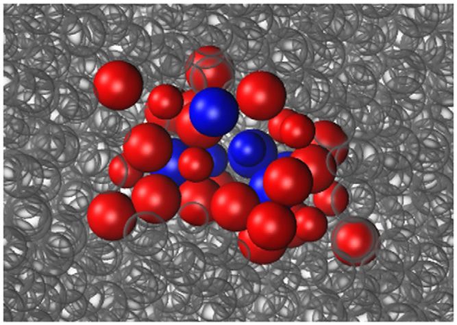
mechanisms is shown in figure 5, where an annealing event, which lowered the structural
energy by 0.79 eV, involved the displacement of 40 atoms more than 0.15 Å, of these, seven
atoms were displaced more than 0.5 Å.
3.2.2. H2 O on the surface of hexagonal ice. A simulation of a molecular system modeled
the diffusion of a water add-molecule on the basal (0 0 0 1) surface of hexagonal ice. As such
systems are of interest to the astronomy community, the simulations were conducted at low
temperatures (Modelling Simul. Mater. Sci. Eng. 22 (2014) 055002 S T Chill et al
Figure 5. A diffusion event in a Cu0.7 Zr0.3 glass crosses an energy barrier of 0.40 eV
and lowers the structural energy by 0.79 eV. The atoms colored blue and red undergo
displacements larger than 0.5 Å and 0.15 Å, respectively, during the event. The small
atoms are Cu and the large atoms are Zr.
-216.9
Energy [eV]
-217.0
-217.1
-217.2
-217.3
Reaction Coordinate
Figure 6. A set of reactions involving a water molecule on an ice surface. Seven events,
overcoming an effective barrier of 0.14 eV results in a rearrangement of the proton
order and the surface energy lowers by 0.28 eV and stabilize due to a more favorable
morphology of the dangling hydrogen atoms.
The average time for such an event at 100 K is on the order of minutes. In the present study, the
empirical TIP4P-flex potential [37] was applied. Figure 6 shows the structural rearrangements
resulting from a series of six event, which lowered the system energy by 0.28 eV. For this
sequence of events to occur, an effective barrier of 0.14 eV was overcome.
3.2.3. Breakup of a boron cluster in bulk silicon. The break-up of a boron cluster in a bulk
silicon lattice was modeled at 500 K using energies and forces from DFT. Boron is commonly
used as a dopant for p-type silicon. The high B concentration required for nanoscale devices
can lead to dopant clustering and deactivation. Thus, the kinetics of dopant cluster formation
and break-up is of interest to the semiconductor industry. The details of the DFT calculation
and how the initial configuration was created have been reported previously [38].
Here we show how on-the-fly coarse graining (MCAMC) [33] and the kinetic database
(KDB) [38] can reduce the computational effort needed to model long timescales. We report
10Modelling Simul. Mater. Sci. Eng. 22 (2014) 055002 S T Chill et al
102
101
100
10-1
Simulation Time (s)
-2
10
10-3
-4
10
10-5
-6
10
-7 AKMC
10
-8 KDB+AKMC
10
MCAMC+KDB+AKMC
10-9
0 2 4 6 8 10
Compuational Time (Cluster-Days)
Figure 7. A comparison of how the kinetic database (KDB) and Monte Carlo with
adsorbing Markov chains (MCAMC) reduce the computation time required to model
the dynamics of a B2 I cluster in bulk Si with AKMC.
a reaction pathway for the break-up of B2 I clusters, the discovery of which was enabled by
using the geometry comparison routines in EON to exploit the symmetry of the system to
greatly reduce the number of identical states that needed to be explored. The KDB reduces
the computational cost of finding new saddles in each state, by reusing information learned in
previous states or simulations. Processes are added to the KDB using a minimal representation
that includes only moving atoms and their immediate environment. The KDB is queried to
provide suggestions of available saddle point geometries. These suggestions accelerate AKMC
simulations by reducing the number of random searches needed to reach confidence that a
sufficient rate table has been determined.
To show the effects of the KDB and MCAMC, three AKMC simulations were run: the
first using both the KDB and MCAMC, the second using only the KDB and a third using
neither acceleration method. For each simulation, the AKMC confidence was set to 0.95,
which corresponds to a stopping criterion in each state where no new event was added to the
rate table within 20 consecutive searches. Each saddle search was initialized by displacing
each degree of freedom of a B atom and all atoms within 2.6 Å by a random number drawn
from a Gaussian distribution with a standard deviation of 0.2 Å.
The results are shown in figure 7. The unit of computational time, a cluster-day, is defined
as one day of CPU time provided by a local cluster containing 39 nodes, each with eight Intel
Xeon X5355 cores running at a clock rate of 2.66 GHz. The use of the KDB reduces the
work needed to explore each state and here it saves more than a day of cluster time. However,
without the use of MCAMC the KMC simulation becomes trapped in a set of states separated
by low barriers. The mean number of steps required to escape this superbasin is 5×10⁹ . The
number of KMC steps that could be performed per second was 3000, which means that it would
have taken 20 cluster-days (on average) to escape from the superbasin each time the simulation
entered it. The use of KDB and MCAMC allowed us to find the full B2 I dissociation pathway
shown in figure 8.
3.3. Basin hopping
BH is an algorithm for determining global minimum energy structures [39]. In BH, a Monte
Carlo (MC) simulation is performed on a transformed PES, Ẽ(X ), obtained from an energy
11Modelling Simul. Mater. Sci. Eng. 22 (2014) 055002 S T Chill et al
2.5
2.0
Energy (eV)
1.5 f
c
d g
1.0
e
0.5
b
a
0
0 2 4 6 8 10 12 14 16 18
Reaction Coordinate (Å)
Figure 8. A reaction pathway for B2 I cluster rearrangement in Si (a)-(c) and dissociation
(d)-(g) found in an AKMC simulation using forces and energies from DFT.
minimization of the atomic configuration X . The standard Metropolis acceptance probability,
Pacc = min[1, exp(−(Ẽ(Xnew ) − Ẽ(Xold ))/kB T )], (6)
is used where Xold and Xnew are the configurations before and after each trial move. MC
moves are made by displacing each coordinate by either a random uniform or Gaussian
distribution. Our implementation also allows for swapping moves, where a pair of atoms
of differing elements have their coordinates exchanged. The size of the displacement can also
be dynamically updated during the simulation to reach a target acceptance ratio [40].
There are several enhancements to BH that have been implemented including significant
structure basin hopping (SSBH) [41] and basin hopping with occasional jumping (BHOJ) [42].
In SSBH all displacements are made from the local minimum of the previous displacement.
In BHOJ, when a predetermined number of MC moves are rejected in a row, a fixed number
of MC moves are performed at infinite temperature. This gives the method a chance to escape
from an energy funnel that doesn’t contain the global minimum.
As an example, we show results from the global optimization of a A42 B58 binary Lennard-
Jones (LJ) cluster with energy given by
( ) *
σαβ 12 σαβ 6
E=4 ϵαβ − , (7)
iModelling Simul. Mater. Sci. Eng. 22 (2014) 055002 S T Chill et al
1.2 1 core
8 cores
16 cores
1.0 512 cores
BOINC ~4000 cores
log(EA - E0)
0.8
0.6
0.4
0.2
0 1 2 3 4 5
Wall Clock Time (hours)
Figure 9. The difference between the lowest energy found by BH simulations (EA ) and
the lowest known global minimum (E0 ) plotted as a function of wall clock time. The
amount of time taken to reach lower energies is reduced as more cores are utilized.
Table 1. Comparison of the rate of escape from the compact Pt heptamer island state
at 400 K using different long timescale methods. The PRD rates are based upon the
mean-first-escape times from four trajectories.
Method Escape rate (s−1 ) Force calls
PRD (7.7 ± 3.8) × 105 1 × 10⁹
PRD/hyperdynamics (6.1 ± 2.3) × 105 1 × 10⁶
AKMC/HTST 8.7 × 10⁵ 2 × 10⁴
4. Discussion
The motivation for developing the EON software is to make different approaches to long
timescale simulations of atomic systems available in an integrated package that can make use
of diverse computational resources. The common toolkit of optimizers, dynamics algorithms,
saddle point finding methods and interatomic potentials allows for a direct comparison of
methods and makes it easier for the user to select the method which best fits the problem at
hand. EON allows for the development of hybrid methods which can take advantage of the
strengths and mitigate the weaknesses of the different algorithms.
An example comparison between methods is given in table 1, in which the rate of escape
from the compact heptamer island configuration (shown in figure 4) is calculated at 400 K
using three different long timescale methods: PRD, PRD combined with hyperdynamics and
HTST as implemented in the AKMC method. Each of these methods exhibit linear speed-
up with respect to the number of CPU cores used so that the wall-clock time to run each
simulation is proportional to the number of force calls divided by the number of cores. On the
previously mentioned 2.66 GHz Xeon X5355 processors, one force call takes about 8 ms on
a single core, so that the HTST calculation takes 2.6 min on 1 core, the PRD/hyperdynamics
calculation takes 16 min on 16 cores and the PRD calculation takes 1.4 days on 64
cores. These wall-clock times closely reflect the conditions under which the simulations
were run.
The escape rate for the compact Pt heptamer island can be estimated with the fewest
force calls using AKMC, where the transition mechanisms are found using saddle point
searches and the rate of each mechanism is calculated using HTST as in equation (1). HTST
13Modelling Simul. Mater. Sci. Eng. 22 (2014) 055002 S T Chill et al
is computationally efficient, but it relies on several assumptions that can contribute systematic
errors to the escape rate. First, some relevant saddle points may not be identified by the
search algorithm, resulting in an incomplete rate table; second, the harmonic approximation
to the TST rate may not be accurate enough at the simulation temperature; and third, the TST
approximation itself may contain errors due to dynamical recrossing events.
To test these approximations, a more accurate estimate of the rate was calculated using
PRD, which relies on fewer assumptions. The equations of motion were integrated with a 2 fs
time step and a dephasing time of 2 ps. The Andersen thermostat was used to sample from the
NVT ensemble with soft collisions, rescaling 20% of the velocity of atoms on a timescale 20 fs.
Table 1 shows that the HTST rate is within the uncertainty of the rate calculated with PRD.
At high enough temperature, the harmonic approximation will break down and the HTST rate
will become less accurate. However, when HTST holds, AKMC is an efficient method, being
orders of magnitude less computationally demanding than PRD. The AKMC approach can
also, in principle, be extended beyond HTST to variationally optimized hyper planar TST, and
could, furthermore, be implemented to include dynamical corrections [44]. Understanding the
tradeoff between computational cost and accuracy of TST calculations beyond the harmonic
approximation are the subject of ongoing studies.
Hyperdynamics is a good compromise between PRD and HTST because it is substantially
faster than PRD when a good bias potential is known, and the systematic errors which can be
introduced with a poor choice of bias potential can be quantified. The PRD/hyperdynamics rate
in table 1 was calculated using the bond-boost bias potential with the parameters described in
section 3.1. The parameters were tuned so that the bias potential smoothly reached zero at the
lowest energy saddle point (0.6 eV) with a maximum fractional bond stretch of 22%. The data
in table 1 shows a hyperdynamics rate in agreement with that of PRD and a thousand-fold gain
in computational efficiency. It should be noted, however, that without the PRD calculation for
reference, the hyperdynamics calculation would have to be repeated with more conservative
settings to check for systematic errors introduced by the bias potential.
While much progress has been made in the development of algorithms for long timescale
simulations, this is still an important challenge to further development and new methods are
being proposed frequently. An essential aspect of this work should be systematic and careful
benchmarking and comparison of the performance of the various approaches, both in terms of
accuracy and computational effort. To further this endeavor, we are developing a community-
based website where authors can publish and compare their methods and codes on benchmark
problems. The benchmark website can be accessed at http://optbench.org/.
The EON code is freely available under the GNU Public License version 3. EON can be
obtained at http://theory.cm.utexas.edu/eon/.
Acknowledgments
The work in Austin was supported by the National Science Foundation (CHE-1152342), the
Welch Foundation (F-1841), the Texas Advanced Computing Center and the National Energy
Research Scientific Computing Center. The work in Iceland was supported by the Icelandic
Research Fund, the University of Iceland Research Fund, and the Nordic High Performance
Computing Center in Iceland. We gratefully acknowledge all the contributors of computer
time to the EON BOINC project and Erik Edelmann (NDGF) for his contributions to the ARC
communicator.
14Modelling Simul. Mater. Sci. Eng. 22 (2014) 055002 S T Chill et al
References
[1] Voter A F 1998 Parallel replica method for dynamics of infrequent events Phys. Rev. B 57 R13985–8
[2] Voter A F 1997 Hyperdynamics: accelerated molecular dynamics of infrequent events Phys. Rev.
Lett. 78 3908–11
[3] Miron R A and Fichthorn K A 2003 Accelerated molecular dynamics with the bond-boost method
J. Chem. Phys. 119 6210–6
[4] Henkelman G and Jónsson H 2001 Long time scale kinetic Monte Carlo simulations without lattice
approximation and predefined event table J. Chem. Phys. 115 9657–66
[5] Wales D J and Doye J P K 1997 Global optimization by basin-hopping and the lowest energy
structures of Lennard-Jones clusters containing up to 110 atoms J. Phys. Chem. A 101 5111–6
[6] Goedecker S 2004 Minima hopping: an efficient search method for the global minimum of the
potential energy surface of complex molecular systems J. Chem. Phys. 120 9911–7
[7] Anderson D P 2004 Boinc: a system for public-resource computing and storage 5th IEEE/ACM
Int. Workshop on Grid Computing (Pittsburgh, PA) pp 4–10
[8] Cai X, Langtangen H P and Moe H 2005 On the performance of the python programming language
for serial and parallel scientific computations Sci. Program. 13 31–56
[9] Jónsson H, Mills G and Jacobsen K W 1998 Nudged elastic band method for finding minimum
energy paths of transitions Classical and Quantum Dynamics in Condensed Phase Simulations
ed B J Berne et al (Singapore: World Scientific) pp 385–404
[10] Bitzek E, Koskinen P, Fähler F, Moseler M and Gumbsch P 2006 Structural relaxation made simple
Phys. Rev. Lett. 97 170201
[11] Hestenes M R and Steifel E 1952 Methods of conjugate gradients for solving linear systems J. Res.
Natl Bur. Stand. 49 409–36
[12] Nocedal J 1980 Updating quasi-Newton matrices with limited storage Math. Comput. 35 773–82
[13] Plimpton S 1995 Fast parallel algorithms for short-range molecular dynamics J. Comput. Phys.
117 1–19
[14] Kresse G and Hafner J 1993 Abinitio molecular dynamics for liquid metals Phys. Rev. B
47 R558–61
[15] Mortensen J J, Hansen L B and Jacobsen K W 2005 Real-space grid implementation of the projector
augmented wave method Phys. Rev. B 71 035109
[16] Daw M S and Baskes M I 1984 Embedded-atom method: derivation and application to impurities,
surfaces, and other defects in metals Phys. Rev. B 29 6443–53
[17] Voter A F and Chen S P 1987 Accurate interatomic potentials for Ni, Al and Ni3 Al Mater. Res. Soc.
Symp. Proc. 82 175–80
[18] Jacobsen K, Stoltze P and Nørskov J K 1996 A semi-empirical effective medium theory for metals
and alloys Surf. Sci. 366 394–402
[19] Lenosky T J, Sadigh B, Alonso E, Bulatov V V, Diaz de la Rubia T, Kim J, Voter A F and Kress J D
2000 Highly optimized empirical potential model of silicon Modelling Simul. Mater. Sci. Eng.
8 825
[20] Tersoff J 1988 Empirical interatomic potential for silicon with improved elastic properties Phys.
Rev. B 38 9902
[21] Justo J F, Bazant M Z, Kaxiras E, Bulatov V V and Yip S 1998 Interatomic potential for silicon
defects and disordered phases Phys. Rev. B 58 2539
[22] Jorgensen W L, Chandrasekhar J, Madura J D, Impey R W and Klein M L 1983 Comparison of
simple potential functions for simulating liquid water J. Chem. Phys. 79 926–35
[23] Vtsttools 2012 http://theory.cm.utexas.edu/vtsttools
[24] EON 2012 distributed computing project http://eon.ices.utexas.edu/
[25] Nordugrid 2012 www.nordugrid.org/arc/
[26] Zhang L, Chill S T and Henkelman G 2014 Distributed replica dynamics in preparation
[27] Voter A F 2007 Introduction to the kinetic Monte Carlo method Radiation Effects in Solids (NATO
Science Series II: Mathematics, Physics and Chemistry) ed K E Sickafus et al (Amsterdam:
Springer) pp 1–23
15Modelling Simul. Mater. Sci. Eng. 22 (2014) 055002 S T Chill et al
[28] Henkelman G and Jónsson H 1999 A dimer method for finding saddle points on high dimensional
potential surfaces using only first derivatives J. Chem. Phys. 111 7010–22
[29] Horn R A and Johnson C R 1985 Matrix Analysis (Cambridge: Cambridge University Press)
[30] Munro L J and Wales D J 1999 Defect migration in crystalline silicon Phys. Rev. B 59 3969
[31] Malek R and Mousseau N 2000 Dynamics of Lennard-Jones clusters: a characterization of the
activation-relaxation technique Phys. Rev. E 62 7723–8
[32] Xu L and Henkelman G 2008 Adaptive kinetic Monte Carlo for first-principles accelerated dynamics
J. Chem. Phys. 129 114104
[33] Novotny M A 1995 Monte carlo algorithms with absorbing Markov chains: fast local algorithms
for slow dynamics Phys. Rev. Lett. 74 1–5
[34] Grinstead C M and Snell J L 2003 Introduction to Probability 2nd edn (Providence, RI: American
Mathematical Society)
[35] Pedersen A, Berthet J C and Jónsson H 2012 Simulated annealing with coarse graining and
distributed computing Lect. Notes Comput. Sci. 7134 34–44
[36] Mendelev M I, Sordelet D J and Kramer M J 2007 Using atomistic computer simulations to analyze
x-ray diffraction data from metallic glasses J. Appl. Phys. 102 043501
[37] Lawrence C P and Skinner J L 2003 Flexible TIP4P model for molecular dynamics simulation of
liquid water Chem. Phys. Lett. 372 842–7
[38] Terrell R, Welborn M, Chill S T and Henkelman G 2012 Database of atomistic reaction mechanisms
with application to kinetic Monte Carlo J. Chem. Phys. 137 015105
[39] Wales D J and Scheraga H A 1999 Global optimization of clusters, crystals, and biomolecules
Science 285 1368–72
[40] Allen M P and Tildesley D J 1987 Computer Simulation of Liquids (Oxford: Oxford Univ. Press)
[41] White R P and Mayne H R 1998 An investigation of two approaches to basin hopping minimization
for atomic and molecular clusters Chem. Phys. Lett. 289 463–8
[42] Iwamatsu M and Okabe Y 2004 Basin hopping with occasional jumping Chem. Phys. Lett.
399 396–400
[43] Sicher M, Mohr S and Goedecker S 2011 Efficient moves for global geometry optimization methods
and their application to binary systems J. Chem. Phys. 134 044106
[44] Jónsson H 2011 Simulation of surface processes Proc. Natl Acad. Sci. 108 944–9
16You can also read