Homodyne-based quantum random number generator at 2.9 Gbps secure against quantum side-information - Nature
←
→
Page content transcription
If your browser does not render page correctly, please read the page content below

ARTICLE
                  https://doi.org/10.1038/s41467-020-20813-w                OPEN

                  Homodyne-based quantum random number
                  generator at 2.9 Gbps secure against quantum
                  side-information
                  Tobias Gehring 1,5 ✉, Cosmo Lupo2,3,5, Arne Kordts1, Dino Solar Nikolic1, Nitin Jain1, Tobias Rydberg1,
                  Thomas B. Pedersen4, Stefano Pirandola 2 & Ulrik L. Andersen 1 ✉
1234567890():,;

                  Quantum random number generators promise perfectly unpredictable random numbers. A
                  popular approach to quantum random number generation is homodyne measurements of the
                  vacuum state, the ground state of the electro-magnetic field. Here we experimentally
                  implement such a quantum random number generator, and derive a security proof that
                  considers quantum side-information instead of classical side-information only. Based on the
                  assumptions of Gaussianity and stationarity of noise processes, our security analysis fur-
                  thermore includes correlations between consecutive measurement outcomes due to finite
                  detection bandwidth, as well as analog-to-digital converter imperfections. We characterize
                  our experimental realization by bounding measured parameters of the stochastic model
                  determining the min-entropy of the system’s measurement outcomes, and we demonstrate a
                  real-time generation rate of 2.9 Gbit/s. Our generator follows a trusted, device-dependent,
                  approach. By treating side-information quantum mechanically an important restriction on
                  adversaries is removed, which usually was reserved to semi-device-independent and device-
                  independent schemes.

                  1 Centerfor Macroscopic Quantum States (bigQ), Department of Physics, Technical University of Denmark, Fysikvej, 2800 Kgs. Lyngby, Denmark.
                  2 Department  of Computer Science, University of York, York YO10 5GH, UK. 3 Department of Physics and Astronomy, University of Sheffield,
                  Sheffield, UK. 4 Cryptomathic A/S, Åboulevarden 22, 8000 Aarhus C, Denmark. 5These authors contributed equally: Tobias Gehring, Cosmo Lupo.
                  ✉email: tobias.gehring@fysik.dtu.dk; ulrik.andersen@fysik.dtu.dk

                  NATURE COMMUNICATIONS | (2021)12:605 | https://doi.org/10.1038/s41467-020-20813-w | www.nature.com/naturecommunications                       1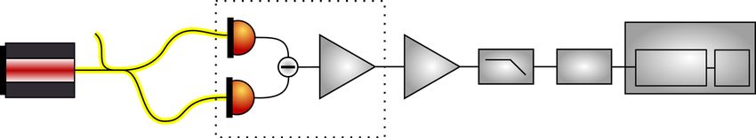
ARTICLE                                                                  NATURE COMMUNICATIONS | https://doi.org/10.1038/s41467-020-20813-w

R
       andom numbers are ubiquitous in modern society1. They                  information theoretically secure Toeplitz randomness extractor
       are used in numerous applications ranging from crypto-                 have been demonstrated recently12,18–20,22. Previously reported
       graphy, simulations, and gambling, to fundamental tests of             QRNG implementations achieved only moderate speeds or did
physics. For most of these applications, the quality of the random            not extract random numbers in real time6–8,11,13–17.
numbers is of utmost importance. If, for instance, cryptographic                 Here we devise a security analysis for QRNGs based on
keys originating from random numbers are predictable, it will                 quadrature measurements of the (trusted) vacuum state that takes
have severe consequences for the security of the internet. To                 quantum side information into account. Our security analysis is
ensure the security of cryptographic encryption, the random                   based on the assumptions of stationarity and Gaussianity of the
numbers used to generate the secret encryption key must be                    involved noise processes. We include correlations of measure-
completely unpredictable, private, and their randomness must be               ment outcomes in the security proof as well as the imperfections
certified.                                                                     of analog-to-digital conversion. We experimentally implement
   True unpredictability and privacy of the generated numbers                 the QRNG and use a conservative and rigorous approach to
can be attained through a quantum measurement process: by                     characterize the parameters of the stochastic model that deter-
performing a projective measurement on a pure quantum state,                  mines the amount of randomness. To establish a conservative
and ensuring that the state is not an eigenstate of the measure-              bound with confidence intervals on the amount of vacuum
ment projector, the outcome is unpredictable and thus true                    fluctuations, we devise an experimental procedure based on a
random numbers can be generated2. Moreover, the generated                     measurement of the transfer function (TF) of the measuring
numbers can be private since a pure state cannot be correlated to             device. Using real-time Toeplitz randomness extraction imple-
any other state in the universe.                                              mented in an FPGA, we achieve a rate of 2.9 Gbit/s.
   Numerous different types of quantum random number gen-
erators (QRNGs) have been devised exploiting the quantum                      Results
uncertainty in photon counting measurements, phase measure-                   Setting the stage. A schematic of our QRNG is shown in Fig. 1.
ments, or quadrature measurements3–5. One particular approach of              An arbitrary quadrature of the vacuum state is measured using a
increasing interest due to its high practicality is the optical quad-         balanced homodyne detector comprising a bright reference beam,
rature measurements of the vacuum state by means of a simple                  a nominal symmetric beam splitter, and two photo diodes23. The
homodyne detection6–8. This approach combines simplicity, cost-               measurement outcomes ideally are random with a Gaussian
effectiveness, chip integrability, and high generation speed.                 distribution associated with the Gaussian Wigner function of the
   State-of-the art security proofs for such QRNGs assumed that               vacuum state24. The measured distribution, however, contains
the information available in the environment about the mea-                   two additional independent noise sources: excess optical noise
surement outcomes, so-called side information, is of classical                and electronic noise, thereby contributing two side channels.
nature8. Recently, quantum side information was taken into                    These must be accounted for in estimating the min-entropy of the
account for a source-independent QRNG9–12, which however                      source.
requires a more complex measurement apparatus.                                   The amount of quantum randomness that can be extracted
   Furthermore, it has been assumed in the security proof that                from the homodyne measurement of vacuum fluctuations is given
subsequent measurement outcomes of QRNGs based on homo-                       by the leftover hash lemma against quantum side information25,26
dyning of vacuum states are uncorrelated in time. Therefore,                                                             1
experiments dealt with the unavoidable correlations caused by the                                ‘ ≥ NH min ðXjEÞ  log 2 :                ð1Þ
finite bandwidth of the detection system by exploiting aliasing in                                                      2ϵhash
the sampling procedure or by using suitable post-processing                   Here H min ðXjEÞ is the min-entropy of a single measurement
algorithms6–8,11,13–20. Such measures usually throttle the overall            outcome drawn from a random variable X conditioned on the
rate considerably or remove the correlations only partially.                  quantum side information E, N is the number of aggregated
   A rigorous characterization of the system is of utmost impor-              samples, and ϵhash is the distance between a perfectly uniform
tance as any parameter uncertainty introduces a non-zero prob-                random string and the string produced by a randomness
ability for system failure, i.e., the probability that the actual device      extractor. It is therefore clear that we need to find the min-
does not follow the stochastic model describing the underlying                entropy of our practical—thus imperfect—realization in order to
physical random number generation process. Knowing the failure                bound the amount of randomness. We achieve this in a two-step
probability for the system is critical to its certification. Previously        approach: First, we theoretically derive a bound for the min-
this metrology-grade approach was used for phase fluctuation                   entropy using a realistic model and express it in terms of
QRNGs21. This includes that imperfect analog-to-digital con-                  experimentally accessible parameters. Second, we experimentally
version is taken into account.                                                deduce these parameters through a conservative and rigorous
   Real-time field-programmable-gate-array (FPGA) imple-                       characterization. Using such an approach, we find the worst-case
mentations of randomness extraction with Gbit/s-speed using an                min-entropy compatible with the confidence intervals of our

Fig. 1 Schematic of the quantum random number generator. A 1.6 mW 1550 nm laser beam was split into two by a 3 dB fiber coupler and detected by a
home-made homodyne detector based on an MAR-6 microwave amplifier from Minicircuits and two 120 μm indium–gallium–arsenide photo diodes (PD).
The output of the detector was amplified with another microwave amplifier, low pass filtered at 400 MHz, and digitized with a 16 bit 1-GSample/s analog-
to-digital converter (ADC). The ADC output was read by a Xilinx Kintex UltraScale field-programmable gate array (FPGA). The ADC and FPGA were
hosted by a PCI Express card from 4DSP (Abaco). The FPGA was used for real-time randomness extraction based on Toeplitz hashing. Random access
memory (RAM) was used to store the output.

2                 NATURE COMMUNICATIONS | (2021)12:605 | https://doi.org/10.1038/s41467-020-20813-w | www.nature.com/naturecommunications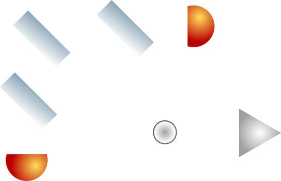
NATURE COMMUNICATIONS | https://doi.org/10.1038/s41467-020-20813-w                                                                                ARTICLE

characterization and calibration measurements, thereby obtaining                  The outcome X of homodyne detection on a thermal state with
a string of ϵ-random bits that are trustworthy with the same level              mean photon number n is a continuous real-valued variable,
of confidence.                                                                   whose probability density distribution is
                                                                                                     pX ðxÞ ¼ Gðx; 0; g 2 ð1 þ 2nÞÞ ;                  ð3Þ
Theoretical analysis. The theoretical analysis of the security of
the QRNG is made under the following assumptions:                               where g is a gain factor and
                                                                                                                     1          ðxμÞ2
   A0 The predictions of quantum mechanics are reliable.                                           Gðx; μ; v2 Þ ¼ pffiffiffiffiffiffiffiffiffiffi e 2v2            ð4Þ
   A1 The measurement performs homodyne detection on a                                                              2πv   2

   single-mode and the measurement outcome is linear in the                     denotes a Gaussian in the variable x, with mean μ, and variance v2.
   quadratures.                                                                    In our QRNG, the continuous variable X is mapped into a
   A2 The quantum state that is measured is a single mode                       discrete and bounded variable X   due to the use of an ADC with
   thermal state with stationary mean photon number.                            range R and bin size Δx. We therefore consider a model in which
   The analysis of the QRNG follows a device-dependent                                                                that assumes values j = 1, 2,
                                                                                X is replaced by a discrete variable X
approach, which assumes that the system (and therefore the                      …, d with probability mass distribution
min-entropy of the source) does not change after system                                                         Z
characterization (A2). The quantum side information comprises                                          pX ðjÞ ¼    dxpX ðxÞ ;                   ð5Þ
                                                                                                                          Ij
all information that can be extracted from the environment of the
QRNG, i.e., from the rest of the universe. Therefore, under                     where Ijs are d intervals that discretize the outcome of homodyne
assumptions A0–A2, the bits extracted by the QRNG are random                    detection. This models an ideal ADC without errors.
with respect to all (quantum and classical) side channels.                        The correlations between the discretized outcome X      and the
Following A2, homodyne detection is performed on a single                       environment E are described by the classical-quantum (CQ) state,
optical mode in a thermal state, which at a given time is                                                  X                      ðjÞ
characterized by the field quadratures ^q and ^p.                                                    ρXE ¼       pX ðjÞj jih jj  ρE ;          ð6Þ
   The physical model of our device is derived in “Methods.”                                                      j

There we show that our device performs the measurement                          with
                                                                                                                        Z
                                         ^ ;
                                   ^ a þ NÞ                                                           ðjÞ       1
                            ^q ¼ gðX                                    ð2Þ                          ρE     ¼                  dx pX ðxÞρxE :          ð7Þ
                                                                                                              pX ðjÞ      Ij

where g is a gain factor, X ^ a is the quadrature operator of the               Here j ji are orthogonal states representing the possible discrete
vacuum mode entering the central beam splitter, and N ^ is a noise              outcomes and ρxE describes the post-measurement quantum state
operator describing all noise sources.                                          of the environment. The explicit expressions of these quantities
   In the following, we first present a theoretical analysis of a                are given in “Methods,” and the full derivation is in Supplemen-
source emitting i.i.d. (independent and identically distributed)                tary Note 2.
quantum states, i.e., a source of infinite bandwidth, and an ideal                  We will now quantify the rate of the QRNG in terms of the
analog-to-digital converter (ADC). We then extend the security                  conditional min-entropy with quantum side information. Given
analysis to imperfect ADCs. Finally, we extend to a source with                                                               conditioned on the
                                                                                the state ρXE in Eq. (6), the min-entropy of X
finite bandwidth that emits correlated (non-i.i.d.) quantum states               environment mode reads28
at different times.                                                                                          h                         i
                                                                                                 ρ ¼ sup log k γE1=2 ρ γ1=2
                                                                                         H min ðXjEÞ                                k1 ;       ð8Þ
                                                                                                                           XE E
                                                                                                             γE
Limit of identical and independent distribution. Under ideal
conditions, homodyne detection would allow us to measure the                    where ∥⋅∥∞ denotes the operator norm, i.e., the largest eigenvalue,
quadrature of a target optical mode, which in our setting is in the             and the supremum is over a density operator γE for the
vacuum state. However, as discussed in detail in “Methods,”                     environment system. Here γE ρXE γE
                                                                                                                     1=2      1=2
                                                                                                                                    ¼ I X  γE
                                                                                                                                              1=2
because of experimental imperfections, this vacuum signal is
                                                                                            1=2
mixed with noise. Therefore, the non-ideal homodyne detector                    ρXE I X  γE      , where IX is the identity operator on X. The log
measures the quadrature ^q of a mode, denoted in the following as               has base 2.
S, that is not in the vacuum state. Following assumption A2, said                  In “Methods,” we compute a lower bound on this quantity
state is a thermal state, which we denote as ρS. We recall that a               following a particular choice for γE. The final result (which
thermal state is uniquely characterized by the mean photon                      includes an optimization over the gain g—see “Methods” for the
number n.                                                                       unoptimized result) is
   We require the random numbers to be statistically independent
of any quantum or classical side information. Therefore, we need                                      ≥  log ΓðnÞ erf Δx
                                                                                              H min ðXjEÞ                             ;         ð9Þ
to analyze the correlations between the measured system S and its                                                              2g0
environment E. Following A0, the joint state of S and E is
                                                                                where
necessarily a pure state, ψSE, as the combined system SE is by
                                                                                                                      pffiffiffi pffiffiffiffiffiffiffiffiffiffiffi   2
definition isolated27. There exist infinitely many purifications ψSE                                     ΓðnÞ ¼           nþ nþ1                 ;       ð10Þ
of the thermal state ρS. However, these purifications are all
equivalent up to local unitary transformations in the environment               and g 0 is implicitly defined by the equation

E, and thus they all have the same information content27. To                                               Δx     1      R
perform our theoretical analysis, it is therefore sufficient to                                        erf        ¼ erfc 0 :                           ð11Þ
                                                                                                           2g 0  2      g
consider any of these purifications. We choose the two-mode
squeezed vacuum (TMSV), which is a two-mode Gaussian state
that purifies the thermal state24. The environment E is thus                     ADC digitization noise. The above result assumed an ADC
described by a single bosonic mode.                                             without digitization errors and noise. However, those imperfections

NATURE COMMUNICATIONS | (2021)12:605 | https://doi.org/10.1038/s41467-020-20813-w | www.nature.com/naturecommunications                                 3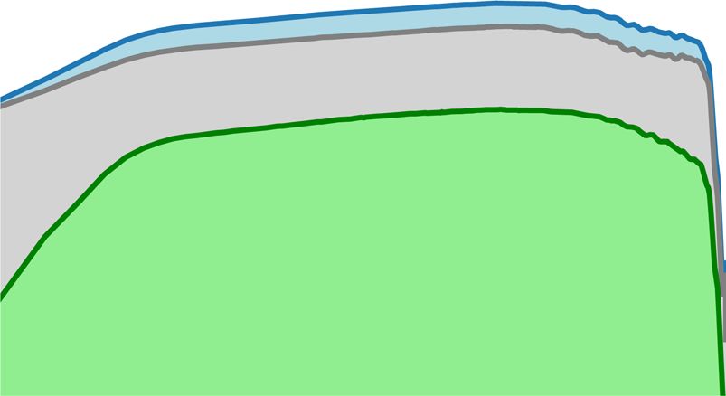
ARTICLE                                                                     NATURE COMMUNICATIONS | https://doi.org/10.1038/s41467-020-20813-w

reduce the extractable min-entropy. Given the true digitization                   where
outcome j, the noise replaces it with a different, possibly random,                                                R 2π dλ
                                                                                                               1           log ½2πef U ðλÞ
output f. For any given f, we count up to M possible true values j                                     σ 2U ¼    2 0 2π                          ð16Þ
                                                                                                             2πe
that map into f. In “Methods,” we show that this reduces the min-
entropy by at most log M bits, i.e.,                                              is the conditional variance of the excess noise.
                                                                                     Because of the finite bandwidth of the measuring apparatus,
                         ≥ H min ðXjEÞ
                 H min ðXjEÞ        ideal  log M ;                     ð12Þ     both the homodyne outcome Xt and excess noise Ut, at a given
                                                                                  time t, are correlated with their values at previous times. To filter

with H min ðXjEÞ
                  ideal
                          given in Eq. (9).                                       out the effects of these correlations, we consider the probability
                                                                                  density distribution of Xt, conditioned on all past homodyne
Beyond i.i.d.: stationary Gaussian process. We now consider the                   measurement outcomes,
more realistic scenario of finite bandwidth. In the experimental
                                                                                                     pX t ðxt jx < t Þ ¼ Gðxt ; μt ; σ 2X Þ ;              ð17Þ
implementation, the finite detection bandwidth, described by the
impulse response of the detector, defines the temporal mode of                     where xt denotes the possible values of the variable Xt at time t,
the measured quantum state. Correlations arise due to the tem-                    x
NATURE COMMUNICATIONS | https://doi.org/10.1038/s41467-020-20813-w ARTICLE
conservative, and thus reliable, estimate of the min-entropy, it is
important that the measurement of these parameters does not
rely on any ideality assumptions of the homodyne detector.
The first two parameters σ2 and σ 2X can be directly established
from the PSD fX(λ) of the homodyne measurement outcomes.
The excess noise parameter σ 2U is, however, more involved as its
amount is determined by several sources whose individual
contributions is too cumbersome to determine. Our goal is thus
to establish the PSD of the excess noise fU(λ) by determining the
contribution of the vacuum fluctuations to the total noise. σ 2U can
then be computed from fU(λ) = fX(λ) − fvac(λ), where fvac(λ) is the
PSD of the vacuum fluctuations.
To establish a lower bound on fvac(λ), we basically consider the
homodyne detector as a box (see Fig. 3a) with a quantum state
Fig. 2 Min-entropy versus the conditional quantum signal-to-noise ratio. input and an input–output relation given by Eq. (2) with
Min-entropy for 8-, 12-, and 16-bit analog-to-digital converter (ADC) unknown parameters. Our strategy is thus to measure the TF of
resolution versus the ratio of conditional variance of the vacuum the box by probing it with known quantum states and to use this
fluctuations and the conditional variance of the excess noise, ðσ 2X σ 2U Þ=σ 2U . result to conservatively calibrate the PSD of the vacuum
Here σ 2X and σ 2U are the conditional variance of the measurement outcomes fluctuations. This method allows us to establish a lower bound
and of the excess noise, respectively. The shaded areas indicate the regions on the vacuum fluctuations under all experimental conditions, in
between low correlations (σ 2X =σ 2 ¼ 0:99), upper trace and high particular where other noise sources couple into the detector, e.g.,
correlations (σ 2X =σ 2 ¼ 0:1), lower trace. Thereby σ2 is the variance of the intensity noise of the laser due to imperfect common-mode
measurement outcomes, which has been optimized to obtain the highest rejection or stray light coupling into the signal port—likely to be
min-entropy. The ADC is assumed to be ideal without digitization errors. an issue with integrated photonic chips.
The TF of the box is measured by injecting a coherent state in
the values for g and n in Eq. (3) are given in Eq. (22) and (24), the form of a second laser beam (independent of the local
respectively. In turn, this allows us to estimate the min-entropy oscillator laser) with low power Psig into the signal port of the
rate using Eq. (9) (see also Eqs. (62) and (67) in “Methods”). This beam splitter as displayed in Fig. 3a. A typical beat signal is
is plotted in Fig. 2 for varying excess noise, ADC resolution, and shown in Fig. 3b obtained by computing an averaged period-
temporal correlations. The x-axis of the plot is the ratio of the ogram from the sampled signal. We record the TF(ν) by scanning
conditional variance of the vacuum fluctuations and the excess the frequency of the signal laser. At each difference frequency ν,
noise, i.e., the quantum noise to excess noise ratio of the virtual i.i. we determine the power of the beat signal and normalize it to Psig.
d. process. If, as assumed for the plot in Fig. 2, the homodyne At high signal-to-noise ratio, the root-mean-square power of the
measurement outcomes and the excess noise have similar beat signal is purely a function of the coherent state amplitude
temporal correlations, this ratio is independent of the amount (determined by the signal laser power). It is independent of the
of correlations. The amount of correlations present in the system noise of the detector, since the second term in Eq. (2), the noise
is instead characterized by the ratio σ 2X =σ 2 , which takes the value term, can be neglected. The first term depending on the
of 1 for an i.i.d. process and becomes smaller for increasing quadrature operator X ^ a can be decomposed into a dominating
temporal correlations. For each ADC resolution, the upper traces term depending on the coherent state amplitude and a negligible
in Fig. 2 show the extractable min-entropy when almost no term depending on the noise of the input state, rendering the
correlations are present. Obviously, stronger correlations yield root-mean-square power independent of the laser noise
lower randomness. properties.
Similar to the result for classical side information8, we show Since the vacuum noise was amplified to optimally fill the
that random numbers can in principle be generated for noise range of the ADC, we used a 20-dB electrical attenuator with flat
treated as quantum side information as well and even in the large attenuation over the frequency band of interest to avoid
excess noise regime. This is due to the fact that relatively small saturation, see Fig. 3a. The result of the TF characterization,
vacuum fluctuations can give a substantial contribution to the normalized to a maximum gain of 1, is shown in Fig. 3c.
entropy if the ADC resolution is sufficiently high. This property is Given the linearity of the detector (A1), we obtain the PSD of
preserved even when a large amount of temporal correlations is the vacuum fluctuations by multiplying the TF(ν) with the shot
present in the recorded data (lower traces in Fig. 2). However, as noise energy hωL contained in 1 Hz bandwidth, where h is
discussed below, increasing the precision may not necessarily lead Planck’s constant and ωL is the angular frequency of the local
to an increase in the min-entropy in the presence of digitization oscillator laser. By modeling the inner workings of the box, we
errors. confirm in Supplementary Note 5 that with this procedure we
indeed obtain a lower bound on the PSD of the vacuum
fluctuations.
System characterization. To be able to apply the theoretical The conservatively estimated PSD of the vacuum fluctuations is
result obtained above to our experimental implementation, we shown in Fig. 4a together with the actually measured PSD of the
need to provide evidence that our implementation indeed fulfills signal. The spectra are clearly colored which indicates that the
the assumptions. This is in fact a difficult task and a detailed data samples are correlated and therefore non-i.i.d. This is further
discussion can be found in “Methods.” corroborated in Fig. 4b, where the autocorrelation of the
We are now in a position to estimate the min-entropy through homodyne measurement outcomes is plotted. It justifies the
characterization of our set-up. According to the theoretical importance of using the min-entropy relation associated with
analysis, the min-entropy can be found by determining the non-i.i.d. samples.
variance σ2 as well as the conditional variances of the homodyne From the PSDs, we calculate the three parameters for obtaining
measurement outcomes σ 2X and the excess noise σ 2U . To obtain a the min-entropy, which are summarized in Table 1. By
NATURE COMMUNICATIONS | (2021)12:605 | https://doi.org/10.1038/s41467-020-20813-w | www.nature.com/naturecommunications 5ARTICLE NATURE COMMUNICATIONS | https://doi.org/10.1038/s41467-020-20813-w Fig. 3 Characterization of the transfer function of the detection system to obtain the vacuum fluctuation noise level. a Experimental set-up for the characterization. VATT variable optical attenuator, PD photo diode, ADC analog-to-digital converter, FPGA field-programmable gate array, RAM random access memory. b Power spectrum from a typical measurement. The transfer function is determined by the amplitude of the beat note. c Transfer function of the homodyne detector and the electronics including the analog-to-digital converter. Inset: transfer function with linear frequency scale. Fig. 4 Experimental results. a The figure shows the power spectral densities (PSDs) of the measurement outcomes, the calibrated vacuum fluctuations (obtained by the system characterization), and the excess noise (obtained by subtracting the PSD of the vacuum fluctuations from the PSD of the measurement outcomes). b Autocorrelation coefficients calculated from the measured samples and averaged 1000 times. The inset shows a zoom. c Relative frequency of the digitization error of the analog-to-digital converter (ADC) with respect to the digitization results. The non-linearity and digitization noise of the ADC leads to a large reduction of the min-entropy. 6 NATURE COMMUNICATIONS | (2021)12:605 | https://doi.org/10.1038/s41467-020-20813-w | www.nature.com/naturecommunications
NATURE COMMUNICATIONS | https://doi.org/10.1038/s41467-020-20813-w                                                                                                          ARTICLE

 Table 1 Summary of the parameters determined by system
 characterization.

 Parameter                                                    Value
 σ2                                                           3.96 × 10⁷ ± 0.09 × 10⁷
 σ 2X                                                         3.29 × 10⁷ ± 0.07 × 10⁷
 σ 2U                                                         2.49 × 10⁷ ± 0.06 × 10⁷
 Conditional quantum to excess noise ratio                    −4.9 dB
 Temporal correlations σ 2X =σ 2                              0.83
 Min-entropy, ideal ADC                                       10.74 bit
 Reduction due to ADC digitization error                      7.23 bit
 Min-entropy                                                  3.51 bit                                  Fig. 5 Physical model of the QRNG showing the involved modes. The local
 Calculated secure length                                     1027 bit
                                                                                                        oscillator described by the mode ^b interferes with the vacuum state
 Extracted length                                             1024 bit
                                                                                                        described by mode ^a at a beam splitter with reflectivity 21 þ Δ. The photo
 Variance of the measurement outcomes σ2, the conditional variance of the measurement                   diode efficiencies are modeled as beam splitters with transmittivities η1 and
 outcomes σ 2X , and the conditional variance of the excess noise σ 2U with their confidence intervals
 for ϵPE = 10−10. The calculated min-entropy for an ideal analog-to-digital converter (ADC)
                                                                                                        η2, where the output modes from the central beam splitter are interfered
 minimized over the confidence intervals, the reduction due to ADC imperfections with ϵADC =             with vacuum modes ^l1 and ^l2 . The difference of the two photo currents from
 2 × 10⁻⁶, the secure length according to the leftover hash lemma, and the length of the
 extracted random sequence in the experiment.
                                                                                                        photo diodes PD1 and PD2, each generated by the light described by
                                                                                                        conversion factor K, is amplified electronically by hamp, during which
                                                                                                        electronic noise is added to the output of the detector.

minimizing the min-entropy over the confidence set of the
estimated parameters, we obtain 10.74 bit per 16-bit sample with                                        Without limitations to the matrix size, a speed of 3.5 Gbit/s could
a failure probability of ϵPE = 10−10 (i.e., the probability that the                                    be reached. The main limitation to the available min-entropy is
actual parameters are outside the confidence intervals) under the                                        the ADC digitization error.
assumption of an ideal ADC.                                                                                Our QRNG is suited for use in high-speed QKD links, for
   Finally, we characterized the digitization error of our ADC,                                         instance, in GHz clocked discrete variable33 as well as in high-
which is shown in Fig. 4c. The measurement protocol is described                                        speed continuous-variable QKD (CVQKD)34. For Gaussian-
in Supplementary Note 3. The reduction of the min-entropy due                                           modulated CVQKD, the uniform random number distribution
to the digitization error is 7.23 bit with a confidence of 2 × 10⁻⁶ as                                   has to be converted to a Gaussian distribution, which requires a
500,000 measurements have been used to construct the histogram                                          larger random number generation rate. Furthermore, QKD
for each digitization result. Thus this yields a total min-entropy of                                   requires composable security and a guarantee of privacy of the
3.51 bit. This relatively large reduction is due to the fact that our                                   random numbers as provided by our system.
ADC is four-way interleaved and has a large analog bandwidth.                                              Further developments to guarantee reliable operation over a
                                                                                                        long time and to fulfill requirements by certification authorities
                                                                                                        would need to include power-on self-tests and online testing of
Discussion                                                                                              the parameters in the security analysis as well as the generated
We have demonstrated a QRNG based on the measurement of                                                 random numbers. Finally, the removal of the Gaussianity and
vacuum fluctuations with real-time extraction at a rate of 2.9                                           stationarity assumptions in the security analysis, which are in
Gbit/s and security against quantum side information. Our                                               practise difficult to verify, would further strengthen the security of
QRNG has a strong security guarantee with a failure probability                                         the QRNG.
of N 0  ϵhash þ ϵPE þ ϵADC þ ϵseed ¼ N 0  1032 þ 3 ´ 1010 þ 2 ´
106 þ ϵseed , where N 0 is the number of QRNG runs in the past
                                                                                                        Methods
with the same seed for the randomness extractor, ϵhash is the                                           Physical model. Here we will develop a physical model of the QRNG using a
security parameter related to the removal of side information [see                                      description of optical modes by annihilation and creation operators in the Hei-
Eq. (1)], ϵPE = 10−10 is the security parameter of the estimation                                       senberg picture35. A schematic of our detector depicting the involved modes and
of one parameter, ϵADC = 2 × 10⁻⁶ is related to the confidence of                                        parameters is shown in Fig. 5. Mode operators ^a and ^b denote the signal and local
the digitization error measurement, and ϵseed describes the                                             oscillator, respectively. The signal and the local oscillator are mixed at the central
                                                                                                        beam splitter, which, under ideal conditions, has 50% splitting ratio. In our model,
security of the random bits used for seeding the randomness                                             we consider that the splitting ratio of the central beam splitter may deviate from
extractor. Since quantum side information from the past has to be                                       perfect balancing by Δ. The optical modes at the output of the central beam splitter
taken into account, ϵhash grows with time2.                                                             are measured by a pair of photo diodes, with quantum efficiencies η1 and η2,
   We chose ϵhash = 10−32 to keep N 0 ϵhash low enough to, in                                           respectively. The non-unit efficiencies are modeled by introducing the auxiliary
principle, be able to generate Gaussian random numbers with                                             modes ^l1 and ^l2 . Opto-electrical conversion is described by the constant K.
security ϵ = 10−9 for a single execution of a continuous variable                                           The local oscillator laser mode ^b can be written as ^b ¼ h^bi þ δ^b  β þ δ^b,
quantum key distribution (QKD)5 protocol with 1010 transmitted                                          where h^bi is the expectation value and δ^b describes the fluctuations. We operate
                                                                                                        our homodyne detector in the strong local oscillator regime, so that products of
quantum states even after 10 years of continuous operation of the                                       operators describing fluctuations are negligible: δ^xδ^y  0. We note that with local
QRNG. See Supplementary Note 6 for details. We note, however,                                           oscillator photon flux in the range of 1015 the detector operates deep within the
that in our case the ϵ-security parameter is limited by ϵADC. In                                        strong local oscillator regime.
our experiment, the seed bits were chosen with a pseudo-random                                              The modes that are detected by photo detection are given by
number generator, which does not allow us to give a security                                                                         rffiffiffiffiffiffiffiffiffiffiffiffi rffiffiffiffiffiffiffiffiffiffiffiffi !
                                                                                                                              pffiffiffiffiffi   1            1              pffiffiffiffiffiffiffiffiffiffiffiffiffi
guarantee for ϵseed. The generated random numbers passed both                                                            ^c ¼ η1          Δ ^b þ      þ Δ ^a þ 1  η1 ^l1 ;              ð25Þ
                                                                                                                                       2            2
the Dieharder31 and the NIST 800-90B32 statistical batteries of
randomness tests.                                                                                                                   rffiffiffiffiffiffiffiffiffiffiffiffi rffiffiffiffiffiffiffiffiffiffiffiffi !
                                                                                                                           pffiffiffiffiffi    1             1              pffiffiffiffiffiffiffiffiffiffiffiffiffi
   Due to the choice of a very small ϵhash, the real-time speed of                                                     d^ ¼ η2           Δ ^a       þ Δ ^b þ 1  η2 ^l2 :              ð26Þ
                                                                                                                                     2             2
our QRNG was limited to 2.9 Gbit/s by the input size of the
Toeplitz extractor required by our FPGA implementation.

NATURE COMMUNICATIONS | (2021)12:605 | https://doi.org/10.1038/s41467-020-20813-w | www.nature.com/naturecommunications                                                                     7
ARTICLE NATURE COMMUNICATIONS | https://doi.org/10.1038/s41467-020-20813-w
After subtraction and amplification, we obtain As discussed above, the measured state ρS is purified into a TMSV. Thereby the
y second optical mode of this TMSV state, characterized by the field quadratures ^qe
^q ¼ K^c ^c K d^ d^
y ð27Þ and ^pe , is associated with the environment, i.e., the rest of the universe. The TMSV
state is a Gaussian state with zero mean and CM24
^ a þ ~g BX
¼ β~g B þ ~g AX ^ b þ ~g L1 X
^ l1 þ ~g L2 X
^ l2 ð28Þ 0 1
1 ^
h^q2 i qp þ ^p^qi
2 h^ h^q^qe i h^q^pe i
with ~g :¼ Kβ. Here we have introduced the quadrature operators B1 C
B 2 h^p^q þ ^q^pi h^p i
2
h^p^qe i h^p^pe i C
^ a ¼ ^a þ ^ay ;
X ð29Þ V¼B B h^q ^qi
C
C ð43Þ
@ e h^q e
^
pi h^
q 2
e i 1
h^
q
2 e e
^
p þ ^
p ^ i
e e A
q
^ b ¼ δ^b þ δ^by ; ð30Þ h^pe ^qi h^pe ^pi 1 ^ ^ ^^
2 hpe qe þ qe pe i h^pe i
2
X
0 pffiffiffiffiffiffiffiffiffiffiffiffiffiffiffiffiffi 1
^ l1 ¼ ^l1 þ ^ly1 ; ð31Þ 1 þ 2n 0 2 nðn þ 1Þ 0
X B pffiffiffiffiffiffiffiffiffiffiffiffiffiffiffiffiffi C
B 0 1 þ 2n 0 2 nðn þ 1Þ C
¼B
B pffiffiffiffiffiffiffiffiffiffiffiffiffiffiffiffiffi
C:
C ð44Þ
^ l2 ¼ ^l2 þ ^ly2 ;
X ð32Þ @ 2 nðn þ 1Þ 0 1 þ 2n 0 A
pffiffiffiffiffiffiffiffiffiffiffiffiffiffiffiffiffi
and the pre-factors are given by 0 2 nðn þ 1Þ 0 1 þ 2n
1 1 The correlations between the outcome X of ideal homodyne detection and the
B ¼ þ Δ η2 Δ η1 ; ð33Þ quantum side information in its environment are described by the CQ state
2 2
Z
rffiffiffiffiffiffiffiffiffiffiffiffiffiffi ρXE ¼ dx pX ðxÞjxihxj ρxE ; ð45Þ
1
A ¼ η1 þ η2 Δ2 ; ð34Þ
4
where jxi are orthogonal states used to represent the possible outcomes of
sffiffiffiffiffiffiffiffiffiffiffiffiffiffiffiffiffiffiffiffiffiffiffiffiffiffiffiffiffiffiffiffiffiffiffiffiffiffiffi
ffi homodyne detection, and the integral in Eq. (45) extends over the real line. The
1 state ρxE is the conditional state of the environment for a given measurement output
L1 ¼ η 1 1 η 1 Δ ; ð35Þ
2 value x. Without loss of generality, we consider the case where the quadrature ^q is
sffiffiffiffiffiffiffiffiffiffiffiffiffiffiffiffiffiffiffiffiffiffiffiffiffiffiffiffiffiffiffiffiffiffiffiffiffiffiffi measured. We can then compute (see Supplementary Note 1 for details of the
ffi derivation) the first moment of the field quadratures of ρxE :
1
L2 ¼ η2 1 η2 þΔ : ð36Þ pffiffiffiffiffiffiffiffiffiffiffi !
2 h^qe i 2 nðnþ1Þ
¼ gð1þ2nÞ x ; ð46Þ
The homodyne detection circuit implements a high-pass filter that removes the h^pe i 0
first term, which is constant. For an ideal homodyne detector, with Δ = 0 and η1 =
η2 = 1, the output current of the detector reduces to as well as the CM
!
^a :
^q0 ¼ ~g X ð37Þ h^q2e i qe ^pe þ ^pe ^qe i
2 h^
1 1
0
1 ^ ^
¼ 1þ2n
: ð47Þ
All the other terms that appear in Eq. (28) are treated as noise. We define the noise 2 hpe qe þ ^qe ^pe i h^p2e i 0 1 þ 2n
operator, N^ ¼ ðBX^ b þ L1 X
^ l1 þ L2 X
^ l2 Þ=A, and rewrite Eq. (28) as
The continuous variable X is mapped into a discrete and bounded variable X
^a þ N
^q ¼ g X ^ ð38Þ is
due to the use of an ADC. The probability mass distribution of X
Z
with g ¼ ~g A. Note that electronic noise can also be modeled in this way, by pX ðjÞ ¼ dx pX ðxÞ ; ð48Þ
attributing it to fluctuations in the auxiliary modes ^l1 and ^l2 or in the local Ij
oscillator mode δ^b. The goal of the QRNG system is to extract bits from the where Ijs are d intervals that discretize the outcome of homodyne detection. In a
measured homodyne output ^q, with the requirement that these bits are random typical setting, these d non-overlapping intervals Ij are of the form
with respect to the noisy variable N. ^ This requirement means that the extracted
random bits look random to an agent that has perfect knowledge, not only of the I 1 ¼ ð1; R ; ð49Þ
system specifications but also of N. ^ Note that the noise comes from the fluctuations
of the variables X^ b, X
^ l1 , and X
^ l2 and is thus ultimately of quantum nature. For I d ¼ ðR; 1Þ ; ð50Þ
example, an agent may prepare the initial state of the modes ^l1 and ^l2 and measure
and for j = 2, …, d − 1
them after the interaction at the beam splitters shown in Fig. 5.
The finite bandwidth of the detector can be modeled by its impulse response I j ¼ ðaj Δx=2; aj þ Δx=2 ; ð51Þ
hamp, which is the Fourier transform of its frequency response. The output voltage
is then given by with aj = − R + (j − 1)Δx/2 and Δx = 2R/(d − 2). This choice of the intervals
reflects the way in which an ideal ADC with range R and bin size Δx operates in
V out ðtÞ ¼ qðtÞ hamp ðtÞ ; ð39Þ mapping a continuous variable into a discrete one. However, ADCs are not ideal
where * is a convolution. Electronic noise also has finite bandwidth, and we assume devices, and below we show how the digitization error of the ADC reduces the
it to have a Gaussian distribution with PSD Selec(λ), zero mean, and variance min-entropy.
R 2π the correlations with the environment are
In terms of the discrete variable X,
σ 2elec ¼ 0 Selec ðλÞ=2πdλ.
thus described by the state
In our calibration method, described in the main text, we replace the vacuum
X
state in the signal mode ^a with a coherent state. This allows us to estimate the ρXE ¼
ðjÞ
pX ðjÞj jih jj ρE ;
contribution of the vacuum fluctuations, X ^ a , to the PSD of the detector output. ð52Þ
j
with
Theoretical analysis in the i.i.d. limit. Consider a single optical mode char- Z
acterized by the quadrature operators ^q and ^p. For a thermal state ρS with mean ðjÞ 1
ρE ¼ dx pX ðxÞρxE : ð53Þ
photon number n, the first moments of the field quadratures vanish, and the pX ðjÞ Ij
covariance matrix (CM) is
! We are now ready to quantify the rate of the QRNG in terms of the conditional
h^q2 i 1 ^
qp þ ^p^qi conditioned on
2 h^ min-entropy. Given the state ρXE in Eq. (52), the min-entropy of X
V thermal ¼ 1 ð40Þ the eavesdropper (denoted with the letter E) reads28
^^ ^^
2 hpq þ qpi h^p i
2
h i
ρ ¼ sup log k γE1=2 ρ γE1=2 k1 ;
H min ðXjEÞ ð54Þ
1 þ 2n 0 γE
XE
¼ ; ð41Þ
0 1 þ 2n
where ∥⋅∥∞ denotes the operator norm (equal to the value of the maximum
where we, as a matter of convention, put the variance of the vacuum equal to 1. In eigenvalue), and the supremum is over a density operator γE for the environment
^ :¼ tr ðρ OÞ
the equation above, we use hOi ^ for operator O.
^ For such a state, the system.
S
output X of homodyne detection is distributed according to a Gaussian law, Since a direct computation of the min-entropy is not feasible, as it requires an
optimization over all density operators γE in an infinite-dimensional Hilbert space,
pX ðxÞ ¼ Gðx; 0; g 2 ð1 þ 2nÞÞ ; ð42Þ we instead focus on finding a computable lower bound. A first lower bound on the
1=2 1=2
where g is a gain factor. min-entropy is obtained by computing k γE ρXE γE k1 for a given choice of
8 NATURE COMMUNICATIONS | (2021)12:605 | https://doi.org/10.1038/s41467-020-20813-w | www.nature.com/naturecommunicationsNATURE COMMUNICATIONS | https://doi.org/10.1038/s41467-020-20813-w ARTICLE
the state γE, so that we have Note that erf Δx
is a monotonically decreasing function of g 0 with values in [0, 1),
0
1=2 1=2 2g
H min ðXjEÞ ð55Þ
ρ ≥ log k γE ρXE γE k1 1 R
whereas 2 erfc g 0 is monotonically increasing with values in [0, 1/2). This implies
" # that there exists a unique value of g 0 such that
1=2 ðjÞ 1=2
¼ log sup pX ðjÞ k γE ρE γE k1 ; ð56Þ Δx 1 R
j erf 0
¼ erfc 0 : ð71Þ
2g 2 g
where the last equality holds because the eigenstates j ji of ρXE in Eq. (52) are
mutually orthogonal. Here we set γE equal to a Gaussian state with zero mean and If g 0 > g 0 , then Qðg 0 Þ ¼ erf 2g
Δx
0 > Qðg 0 Þ, and if g 0 < g 0 , then
CM Qðg 0 Þ ¼ 12 erfc gR0 > Qðg 0 Þ. This implies that g 0 is a local and global maximum for
1 þ 2ðn þ δÞ 0 the function Q.
; ð57Þ
0 1 þ 2ðn þ δÞ In conclusion, the best lower bound on the conditional min-entropy is
pffiffiffi pffiffiffiffiffiffiffiffiffiffiffi
where the parameter δ will be optimized a posteriori to improve the bound. ≥ log n þ n þ 1 2 log erf Δx
H min ðXjEÞ ; ð72Þ
A second lower bound is obtained by applying the triangular inequality, 2g0
1=2 ðjÞ 1=2
pX ðjÞ k γE ρE γE k1 with g 0 implicitly given in Eq. (71).
Z
1=2 1=2 ð58Þ
¼ k γE dx pX ðxÞ ρxE γE k1
Ij
ADC digitization noise. ADCs are not ideal devices and are subject to digitization
error. We model the digitization error by introducing:
Z
1=2 x 1=2
≤ dx pX ðxÞ k γE ρE γE k1 ; ð59Þ 1. A classical noise variable N, with associated probability distribution pN;
Ij 2. A function f that describes how the noise variable i combines with the
noiseless output value j to produce the noisy output f = f(j, i).
which implies
" Z # Using this model, the quantum side information about the output of the noisy
1=2 x 1=2 ADC is described by the CQ state
H min ðXjEÞ ≥ log sup dx pX ðxÞ k γE ρE γE k1 : ð60Þ X
j Ij ρXEN ¼ pX ðjÞj f ðj; iÞih f ðj; iÞj ρj pN ðiÞjiihij ; ð73Þ
Since ρxE
and γE are both Gaussian states, the above lower bound can be ji
computed using the Gibbs representation techniques developed in ref. 36. where we have introduced a dummy quantum register N to keep track of the noise
Employing these techniques and additional tools, ref. 37 derived a formula for the value i.
min-entropy. By applying this result, we obtain (see Supplementary Note 2 for We want to ensure that the randomness extracted is also independent on the
details) noise variable N, therefore, we compute the min-entropy conditioned on EN,
Z h i
1=2 1=2 1=2 1=2
dx pX ðxÞ k γE ρxE γE k1 ^
H min ðXjENÞ ≥ log γEN ρXEN γEN ð74Þ
Ij 1
Z 2 ð61Þ
1 ðn þ δÞð1 þ n þ δÞ x δ 2 3
¼ pffiffiffiffiffiffiffiffiffiffiffiffiffiffiffiffiffiffiffiffiffiffiffiffiffiffiffiffiffiffiffiffiffiffiffiffiffiffiffiffiffiffiffiffiffiffiffi dx exp : X
g 2πδð2nðn þ 1 þ δÞ þ δÞ Ij 2g 2nðn þ 1 þ δÞ þ δ
2
¼ log 4 pX ðjÞpN ðjÞj f ðj; iÞih f ðj; iÞj
1=2
γEN ρj
1=2
jiihijγEN 5 ð75Þ
To simplify the notation, we define ji 1
rffiffiffiffiffiffiffiffiffiffiffiffiffiffiffiffiffiffiffiffiffiffiffiffiffiffiffiffiffiffiffiffiffiffiffiffiffiffi
4nðn þ 1 þ δÞ þ 2δ 2 3
g 0 :¼ g : ð62Þ X
¼ log 4sup 5;
δ 1=2 1=2
pX ðjÞpN ðiÞγEN ρj jiihijγEN ð76Þ
f ji2Sf
This yields 1
Z Z 2
1=2 1=2 ðn þ δÞð1 þ n þ δÞ x where Sf denotes the setPof values of j, i such that f(j, i) = f.
dx pX ðxÞ k γE ρxE γE k1 ¼ p ffiffiffi dx exp : ð63Þ Putting γEN ¼ γE i pN ðiÞjiihij, we obtain
Ij δg 0 π Ij g02
2 3
For j = 2, …, d − 1, this latter quantity reads X
≥ log 4sup 5
^ 1=2 1=2
Z H min ðXjENÞ pX ðjÞγE ρj γE jiihij ð77Þ
1=2 1=2 f ji2Sf
dx pX ðxÞ k γE ρxE γE k1 1
Ij
ð64Þ 2 3
ðn þ δÞð1 þ n þ δÞ aj Δx aj Δx X
≥ log 4sup 5;
¼ erf 0 þ 0 erf 0 0 1=2 1=2
pX ðjÞγE ρj γE ð78Þ
2δ g 2g g 2g f ;i j2Sf ji
1
ðn þ δÞð1 þ n þ δÞ Δx where Sf∣i is defined as the set of values of j such that f(j, i) = f for a given value of i.
≤ erf ; ð65Þ
δ 2g 0 We further define Jf as the set of values of j such that f(j, i) = f for some value of i.
It is difficult to estimate Sf∣i without making further assumptions on the noise
and for j = 1 and j = d,
underlying the ADC. However, we can experimentally estimate the cardinality ∣Jf∣
Z
1=2 1=2 ðn þ δÞð1 þ n þ δÞ R of the set Jf. Note that Jf contains Sf∣i for all i. We can then write a computable
dx pX ðxÞ k γE ρxE γE k1 ¼ erfc 0 : ð66Þ bound in terms of ∣Jf∣:
Ij 2δ g
2 3
We hence obtain X
^
H min ðXjENÞ 4
≥ log sup
1=2
pX ðjÞγE ρj γE
1=2 5 ð79Þ
≥ log ðn þ δÞð1 þ n þ δÞ Δx 1 R f
H min ðXjEÞ max erf 0
; erfc 0 : ð67Þ j2J f
1
δ 2g 2 g
2 3
We remark that this is in fact a family of lower bounds parameterized by δ and g. X
≥ log 4sup 5
1=2 1=2
The best bound in the family is pX ðjÞ γE ρj γE ð80Þ
f 1
j2J f
≥ min log ðn þ δÞð1 þ n þ δÞ
H min ðXjEÞ
δ δ " #
ð68Þ 1=2 1=2
Δx 1 R ≥ log supjJ f j sup pX ðjÞ γE ρj γE ð81Þ
min log max erf 0
; erfc 0 f j2J f 1
g0 2g 2 g
" #
pffiffiffi pffiffiffiffiffiffiffiffiffiffiffi 2 Δx 1 R 1=2 1=2
¼ log n þ n þ 1 log min0
max erf 0
; erfc 0 : ð69Þ ≥ log supjJ f j sup pX ðjÞ γE ρj γE ð82Þ
g 2g 2 g f j 1
Let us define the function " # " #
Δx 1 R ¼ log sup pX ðjÞ γE
1=2
ρj γE
1=2
log supjJ f j : ð83Þ
QðgÞ :¼ min max erf ; erfc : ð70Þ 1
g0 2g 0 2 g0 j f
NATURE COMMUNICATIONS | (2021)12:605 | https://doi.org/10.1038/s41467-020-20813-w | www.nature.com/naturecommunications 9ARTICLE NATURE COMMUNICATIONS | https://doi.org/10.1038/s41467-020-20813-w
Having established the phase invariance of the measured state, we verify the
Gaussianity of the measured signal. This can only be shown approximately and is
displayed in Fig. 6a where we show the probability quantiles of the measured
samples and compared those to the theoretical quantiles of a Gaussian distribution.
This completes the verification of the assumption in the security proof that a
thermal state is measured.
We are left with that the mean photon number of the thermal state shall be
stationary. Also this can only be proven approximately. We computed the
overlapped Allan deviation of the measurement outcomes, which is shown in
Fig. 6b. It is clearly visible that in the short term the noise processes are stationary.
Over longer times, some fluctuations become evident, which could lead to a lower
min-entropy at times than estimated. A power stabilization of the local oscillator
laser could improve this figure of merit. We, however, leave this investigation for
future work.
Real-time randomness extraction. Having calculated the min-entropy, the next
step is to extract random numbers. This is done by using a strong extractor based
on a Toeplitz matrix hashing algorithm in which the seed can be reused38. We
chose matrix dimensions of n = 5632 bits and m = 1024 bits, which corresponds to
352 input samples with a depth of 16 bit and an output length m < l, chosen such
that Eq. (1) was fulfilled with H min ¼ 3:51 bit and ϵhash < 10−32. The 16-bit samples
provided by the ADC at a rate of 1 GHz are received by the FPGA in chunks of 64
bits at a rate of 250 MHz. For the algorithm implementing the Toeplitz hashing, we
followed the approach of ref. 20. Every clock cycle 64 bits were stored in a block
until n-bits were accepted, after which the next block started receiving data. For
each full block, we carried out the hashing multiplication with bit-wise AND and
subsequent XOR operations on the Toeplitz matrix by first splitting up the matrix
into submatrices of width 16 bit and then shifting the data through the operations.
When the hashing was completed, the m-bit-wide output data was stored in a
register, and the next block was processed. The achieved throughput was 2.9 Gbit/s.
Reporting summary. Further information on research design is available in the Nature
Research Reporting Summary linked to this article.
Fig. 6 Verification of assumption A2. a Quantile–quantile plot indicating Data availability
the Gaussianity of the measured samples. The variance of the samples has All experimental data are available from the authors upon reasonable request.
been normalized to 1. The limited analog-to-digital converter range
truncates the tails of the Gaussian distribution, which results in slight Code availability
deviations from the theoretical quantiles toward the ends. b Overlapped All codes are available from the authors upon reasonable request.
Allan deviation of vacuum state measurements. The stationarity condition
is fulfilled when the experimental points follow the theory curve, which is Received: 30 March 2020; Accepted: 22 December 2020;
the case until about 1000 s where it starts to deviate.
Here the first inequality follows from the fact that Jf contains Sf∣i for all i; the second
inequality follows from the triangular inequality; the third inequality follows from References
the fact that the supremum is larger than the average; and the fourth inequality is 1. Hayes, B. Randomness as a resource. Am. Sci. 89, 300–305 (2001).
obtained by replacing the supremum over j ∈ Jf with the supremum over all values 2. Frauchiger, D., Renner, R. & Troyer, M. True randomness from realistic
of j.
quantum devices. Preprint at https://arxiv.org/abs/1311.4547 (2013).
In conclusion, when compared with an ideal noiseless ADC, the randomness is
3. Ma, X., Cao, Z. & Yuan, X. Quantum random number generation. Quantum
reduced by at most b bits, with b ¼ log ½supf jJf j.
Inf. 2, 16021 (2016).
4. Herrero-Collantes, M. & Garcia-Escartin, J. C. Quantum random number
generators. Rev. Mod. Phys. 89, 015004 (2017).
Verification of assumptions in the theoretical analysis. An integral part is the 5. Pirandola, S. et al. Advances in quantum cryptography. Adv. Opt. Photonics
verification that our implementation indeed fulfills the assumptions made in the 12, 1012–236 (2020).
theoretical analysis of the QRNG. 6. Gabriel, C. et al. A generator for unique quantum random numbers based on
vacuum states. Nat. Photon. 4, 711–715 (2010).
A1. The physical model above verifies that our detector indeed performs homodyne 7. Symul, T., Assad, S. M. & Lam, P. K. Real time demonstration of high bitrate
detection. quantum random number generation with coherent laser light. Appl. Phys.
The condition of the measurement of a single mode are given due to the Lett. 98, 231103 (2011).
following arguments: The local oscillator laser has a side-mode suppression of >70 8. Haw, J. Y. et al. Maximisation of extractable randomness in quantum random
dB and therefore operates in a single frequency mode. The local oscillator number generator. Phys. Rev. Appl. 3, 054004 (2015).
furthermore defines the polarization and the spatial properties (given by the single 9. Cao, Z., Zhou, H., Yuan, X. & Ma, X. Source-independent quantum random
mode fiber) of the measured mode. The temporal properties are given by the number generation. Phys. Rev. X 6, 011020 (2016).
impulse response of the homodyne detector and the following electronic circuits. 10. Marangon, D. G., Vallone, G. & Villoresi, P. Source-device-independent
The linearity of our detector has been tested by connecting the output to an ultra-fast quantum random number generation. Phys. Rev. Lett. 118, 060503
electrical spectrum analyzer instead of the ADC. Varying the power of the signal (2017).
laser in the TF calibration set-up, see Fig. 3, we verified its linear operation. We 11. Avesani, M., Marangon, D. G., Vallone, G. & Villoresi, P. Secure heterodyne-
note that the linearity of the output of the homodyne detection circuit before it is based quantum random number generator at 17 Gbps. Nat. Commun. 9, 5365
sampled by the ADC is the important figure of merit. Nonlinearities introduced by (2018).
the ADC are taken into account separately by the ADC characterization. 12. Drahi, D. et al. Certified quantum random numbers from untrusted light.
Phys. Rev. X 10, 41048 (2020).
A2. The excess noise in the thermal state stems from relative intensity noise of the 13. Fuerst, M. et al. High speed optical quantum random number generation. Opt.
laser and the electronic noise of the homodyne circuit. Both are independent of the Express 18, 13029–37 (2010).
phase between local oscillator and the measured quantum state and can therefore 14. Xu, F. et al. Ultrafast quantum random number generation based on quantum
be modeled as phase invariant state. phase fluctuations. Opt. Express 20, 12366–77 (2012).
10 NATURE COMMUNICATIONS | (2021)12:605 | https://doi.org/10.1038/s41467-020-20813-w | www.nature.com/naturecommunicationsNATURE COMMUNICATIONS | https://doi.org/10.1038/s41467-020-20813-w ARTICLE
15. Nie, Y.-Q. et al. The generation of 68 Gbps quantum random number by 38. Wegman, M. N. & Carter, J. L. New hash functions and their use in
measuring laser phase fluctuations. Rev. Sci. Instrum. 86, 063105 (2015). authentication and set equality. J. Comput. Syst. Sci. 22, 265–279 (1981).
16. Shi, Y., Chng, B. & Kurtsiefer, C. Random numbers from vacuum fluctuations.
Appl. Phys. Lett. 109, 041101 (2016).
17. Abellán, C. et al. Ultra-fast quantum randomness generation by accelerated phase Acknowledgements
diffusion in a pulsed laser diode. Opt. Express 22, 1645–54 (2014). The authors acknowledge support from the Innovation Fund Denmark through the
18. Zhang, X.-G. et al. Fully integrated 3.2 Gbps quantum random Quantum Innovation Center, Qubiz. T.G., A.K., D.S.N., N.J., and U.L.A. acknowledge
number generator with real-time extraction. Rev. Sci. Instrum. 87, 076102 (2016). support from the Danish National Research Foundation, Center for Macroscopic
19. Huang, L. & Zhou, H. Integrated Gbps quantum random number generator Quantum States (bigQ, DNRF142). T.G., N.J., S.P., and U.L.A. acknowledge the EU
with real-time extraction based on homodyne detection. J. Opt. Soc. Am. B 36, project CiViQ (grant agreement no. 820466). C.L. was also supported by the EPSRC
130–136 (2019). Quantum Communications Hub, grant no. EP/M013472/1. The authors thank Alberto
20. Zheng, Z., Zhang, Y., Huang, W., Yu, S. & Guo, H. 6 Gbps real-time optical Nannarelli for valuable discussions.
quantum random number generator based on vacuum fluctuation. Rev. Sci.
Instrum. 90, 043105 (2019). Author contributions
21. Mitchell, M. W., Abellan, C. & Amaya, W. Strong experimental guarantees in T.G., T.B.P., and U.L.A. conceived the idea. T.G. and U.L.A. supervised the project. C.L.
ultrafast quantum random number generation. Phys. Rev. A 91, 012314 and S.P. performed the security analysis with input from T.G. and A.K. T.G., A.K., and
(2015). N.J. conceived and implemented the experiment. T.G. acquired the final data and per-
22. Zhang, X., Nie, Y. Q., Liang, H. & Zhang, J. FPGA implementation of Toeplitz formed data analysis. D.S.N. and T.R. implemented the randomness extraction algorithm
hashing extractor for real time post-processing of raw random numbers. In on FPGA under the supervision of T.G. T.B.P. was responsible for the implementation of
IEEE-NPSS Real Time Conference, (RT) 1–5 (IEEE, 2016). the NIST randomness tests.
23. Shapiro, J. H. Homodyne and heterodyne receivers. IEEE J. Quantum Electron.
QE-21, 237–250 (1985).
24. Weedbrook, C. et al. Gaussian quantum information. Rev. Mod. Phys. 84, Competing interests
621–669 (2012). The authors declare no competing interests.
25. Renner, R. Security of quantum key distribution. Int. J. Quantum. Inf. 6,
1–127 (2008).
26. Tomamichel, M., Schaffner, C., Smith, A. & Renner, R. Leftover Hashing
Additional information
Supplementary information is available for this paper at https://doi.org/10.1038/s41467-
against quantum side information. IEEE Trans. Inf. Theory 57, 5524–5535
020-20813-w.
(2011).
27. Nielsen, M. A. & Chuang, I. L. Quantum Computation and Quantum
Correspondence and requests for materials should be addressed to T.G. or U.L.A.
Information (Cambridge University Press, 2000).
28. Tomamichel, M. A Framework for Non-Asymptotic Quantum Information
Peer review information Nature Communications thanks Xiongfeng Ma and the other
Theory. Ph.D. thesis, ETH Zurich (2012).
anonymous reviewer(s) for their contribution to the peer review of this work.
29. Covers, T. M. & Thomas, J. A. Elements of Information Theor (Wiley-
Interscience, 1991).
Reprints and permission information is available at http://www.nature.com/reprints
30. Gray, R. M. Toeplitz and Circulant Matrices: A Review. Foundations and
Trends in Communications and Information Theory 155–239 (Now
Publisher’s note Springer Nature remains neutral with regard to jurisdictional claims in
Publishers, 2006).
published maps and institutional affiliations.
31. Brown, R. G. Dieharder. http://www.phy.duke.edu/rgb/General/dieharder.php
(2018).
32. Turan, M. S. et al. Recommendation for the entropy sources used for random
bit generation. https://nvlpubs.nist.gov/nistpubs/SpecialPublications/NIST. Open Access This article is licensed under a Creative Commons
SP.800-90B.pdf (2018). Attribution 4.0 International License, which permits use, sharing,
33. Dixon, A. R., Yuan, Z. L., Dynes, J. F., Sharpe, A. W. & Shields, A. J. Gigahertz adaptation, distribution and reproduction in any medium or format, as long as you give
decoy quantum key distribution with 1 Mbit/s secure key rate. Opt. Express 16, appropriate credit to the original author(s) and the source, provide a link to the Creative
18790–18797 (2008). Commons license, and indicate if changes were made. The images or other third party
34. Huang, D., Huang, P., Lin, D., Wang, C. & Zeng, G. High-speed continuous- material in this article are included in the article’s Creative Commons license, unless
variable quantum key distribution without sending a local oscillator. Opt. Lett. indicated otherwise in a credit line to the material. If material is not included in the
40, 3695 (2015). article’s Creative Commons license and your intended use is not permitted by statutory
35. Leonhardt, U. Measuring the Quantum State of Light (Cambridge University regulation or exceeds the permitted use, you will need to obtain permission directly from
Press, 1997). the copyright holder. To view a copy of this license, visit http://creativecommons.org/
36. Banchi, L., Braunstein, S. L. & Pirandola, S. Quantum fidelity for arbitrary licenses/by/4.0/.
Gaussian states. Phys. Rev. Lett. 115, 260501 (2015).
37. Seshadreesan, K. P., Lami, L. & Wilde, M. M. Rényi relative entropies of
quantum Gaussian states. J. Math. Phys. 59, 072204 (2018). © The Author(s) 2021
NATURE COMMUNICATIONS | (2021)12:605 | https://doi.org/10.1038/s41467-020-20813-w | www.nature.com/naturecommunications 11You can also read


