Journal of Sound and Vibration
←
→
Page content transcription
If your browser does not render page correctly, please read the page content below
Journal of Sound and Vibration 482 (2020) 115460

                                                   Contents lists available at ScienceDirect

                                          Journal of Sound and Vibration
                                      journal homepage: www.elsevier.com/locate/jsvi

Characterization of challenges in asymmetric nonlinear
vibration energy harvesters subjected to realistic excitation
Wen Cai, Ryan L. Harne*
Department of Mechanical and Aerospace Engineering, The Ohio State University, Columbus, OH, 43210, USA

a r t i c l e i n f o                                 a b s t r a c t

Article history:                                      With an explosion of the internet of things (IoT), vibration energy harvesting provides an
Received 10 December 2019                             environmentally friendly solution to replace consumable batteries in powering IoT wire-
Received in revised form 17 April 2020                less sensors. Yet, when implemented in practice, ambient vibration input energy is much
Accepted 14 May 2020
                                                      less periodic than assumptions adopted in previous studies. This becomes especially
Available online 19 May 2020
Handling Editor: 2EPAV- Pavlovskaia
                                                      important given that asymmetries are inevitable in nonlinear device platforms. This
                                                      research sheds light on these complex challenges of practical vibration energy harvesting
                                                      by developing and exploring an analytical model based on equivalent linearization. The
Keywords:
Equivalent linearization method
                                                      modeling approach provides an opportunity to understand influences of asymmetry,
Asymmetry                                             nonlinearity, and combined excitation response on the DC power delivery of energy har-
Combined harmonic and stochastic excita-              vesters. In the analytical model, a weighted Gaussian joint distribution is utilized to
tion                                                  approximate the influences caused by the random excitation. Combined with numerical
Nonlinear dynamics                                    and experimental validation, the analysis indicates that with the increase of stochastic
Direct current voltage                                base acceleration, two outcomes are possible. A first outcome involves an enhancement of
                                                      DC power by way of triggering large amplitude nonlinear oscillations. A second outcome
                                                      corresponds to a loss of high power delivery since the noise interferes with the attainment
                                                      of the snap-through dynamic. Either reducing asymmetry or increasing harmonic excita-
                                                      tion component is found to be favorable to induce the power-enhancing dynamics and
                                                      inhibit the occurrence of the second case. Although with the simplified Gaussian distri-
                                                      bution, the analytical framework cannot reproduce exact details of the dynamic responses
                                                      in every case, the results show that the statistical trends of the analysis are overall borne
                                                      out in simulation and experiment. This indicates the new modeling of this research may
                                                      help guide attention to design and deployment techniques for nonlinear vibration energy
                                                      harvesters in practical combined excitation environments, where limitations on precise
                                                      manufacture or placement may introduce structural asymmetry.
                                                                                                          © 2020 Elsevier Ltd. All rights reserved.

1. Introduction

   The extensive network of interconnected wireless devices termed the Internet-of-Things (IoT) has been widely built up in
recent years for applications such as building operations [1], healthcare [2], and smart farming [3], to name a few. The IoT
results in smart, data-informed strategies by continuously collecting and processing trends of user consumption, system
health, and other important metrics. With a projected increase of IoT devices to a trillion by 2025 [4], the high demand on

 * Corresponding author.
   E-mail address: harne.3@osu.edu (R.L. Harne).

https://doi.org/10.1016/j.jsv.2020.115460
0022-460X/© 2020 Elsevier Ltd. All rights reserved.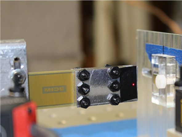
2                                   W. Cai, R.L. Harne / Journal of Sound and Vibration 482 (2020) 115460

disposable batteries suggests a clear threat to the sustainability of our environment and infrastructure. With the decrease of
required power for IoT devices to microwatts [4], vibration energy harvesting can be an environmentally friendly energy
provider of on-demand electrical power due to the high power density and broad availability of kinetic energy [5].
    In recent years, numerous research efforts have been devoted to improving the performance of vibration energy har-
vesting systems. Because of the narrowband characteristic of linear vibration energy harvesters, nonlinear energy harvesting
systems are proposed to meet the requirements of broadband frequency sensitivity and high output power resulting from the
input vibration energy [6e9]. Because of the multistability feature of energy harvesters with particular nonlinearities, a wide
variety of methods have been proposed to readily attain high energy orbit vibration [10e12]. For example, Zhou et al. [12]
proposed a flexible bistable energy harvester with a controllable potential energy function that helps one govern the potential
energy barrier for triggering snap-through vibration. Wang and Liao [11] utilized the load perturbation method to create
strategies that transform system states from intrawell vibration to snap-through oscillation.
    In addition, optimization strategies are applied seeking energy harvesting system designs with maximized performance
[13e15]. Dietl and Garcia [16] employed a gradient search optimization tool to determine that a curved beam shape along the
beam length axis provides optimal and uniform strain distribution for power maximization. Cai and Harne [17,18] utilized the
genetic algorithm optimization method to uncover the entangled influences of nonlinearity, beam shape, and tip mass for
high performing and structurally resilient energy harvesting cantilever designs. Since rectification is necessary to convert the
alternating current (AC) voltage from the piezoelectric beam to direct current (DC) voltage, studies on harvesting circuits
explore methods for maximizing power delivery [19,20]. By utilizing switching strategies with standard rectification, the
synchronous electric charge extraction (SECE) circuit was found to yield a 400% increase in harvested power [21]. On the basis
of the SECE circuit, Lefeuvre et al. [22] presented a phase-shift SECE (PS-SECE) circuit to improve the delivered power up to a
theoretical limit for piezoelectric devices having high electromechanical coupling.
    From this survey of state-of-the-art investigations, one common assumption adopted is the symmetry of potential energy
functions when leveraging nonlinearities for energy harvesting [7,8,17]. Yet, due to factors such as asymmetric magnetic
fields, structure imperfections, or static and gravitational loads, asymmetry is nearly unavoidable in implementing nonlinear
energy harvesting systems. This indicates it is necessary to investigate the influences of asymmetry in the development of
nonlinear energy harvesters. He and Daqaq [23] examined the AC output power of asymmetric nonlinear energy harvesting
systems subjected to pure white noise excitation vibration and indicated that the existence of asymmetry may increase the
output power for a monostable system, whereas the performance of a bistable system is deteriorated. Wang et al. [24]
introduced an installation bias angle to asymmetric bistable energy harvesting systems to reduce negative effects caused by
asymmetric potentials for the energy harvesters when subjected to pure harmonic or random excitation.
    Moreover, pure harmonic or pure stochastic excitation is usually employed in studies to characterize electrodynamic
responses [25,26]. In fact, environments wherein harvesters may be employed to sustain IoT devices may experience complex
vibration conditions such as combined harmonic and stochastic excitation [27,28]. For instance, with the influence of moving
vehicles, the vibrations of bridges show a combined influence of periodic oscillation and random vibration [28]. In order to
analytically predict the dynamical characteristics when subjected to combined harmonic and stochastic excitation, methods
such as Gaussian closure method [29,30], stochastic averaging method [31,32], and equivalent linearization method [33], have
been applied to symmetric Duffing oscillators to statistically characterize the structural dynamics. Yet, due to the complicated
mechanical-electrical coupling in energy harvesters, analytical approaches seldom address DC power delivery that results
following rectification stages. A few insights on this class of structural-electrical coupling have been obtained. For instance,
Kim et al. [34] used numerical approaches to identify the stochastic resonance phenomenon for rotating energy harvesting
systems under combined harmonic and stochastic excitation and validated the findings by experiments. Dai and Harne [35]
introduced an analytical approach to determine the relationship between the electrical and mechanical responses and thus
predict the electromechanical responses of cantilevered energy harvesters due to combined harmonic and stochastic exci-
tation. On the other hand, no works have synthesized a prediction tool for the intricate electromechanical responses of
asymmetric nonlinear vibration energy harvesters subjected to combined vibration excitation conditions. The insight from
such an analytical process would be strongly relevant to help transition energy harvesting devices to practice.
    Motivated to fill the void in understanding, this research investigates the dynamic behaviors of an asymmetric nonlinear
energy harvester integrated with a standard rectification circuit. The aim is to characterize the mechanical and electrical
responses when subjected to combined harmonic and stochastic excitation. In the following sections, an analytical framework
is first established for the proposed system. After validating the system numerically and experimentally, the influences of
asymmetry are investigated considering the combined harmonic and stochastic excitation condition. Finally, a summary of
main findings in the study is provided to conclude this report.

2. Analytical model formulation

   The vibration energy harvesting platform considered in this study is shown in Fig. 1. A piezoelectric cantilever has a tip
mass M0 constructed by the magnet 1 and its holder at the free end. The beam is excited by base motion representative of the
ambient kinetic energy. The electrodes of the beam are interfaced with a standard rectification circuit to convert the AC
voltage to a DC voltage. A pair of repulsive magnets is utilized to introduce nonlinearities into the system. The gap d2 and bias
D between the two magnets determine the magnetic force Fm that governs the type of nonlinearity and the significance of
W. Cai, R.L. Harne / Journal of Sound and Vibration 482 (2020) 115460             3

                                                   Fig. 1. Schematic of nonlinear energy harvesting system.

asymmetry induced into the potential energy profile of the system. The polynomial expression in Eq. (1) is adopted in the
model to approximate the nonlinear magnetic force Fm [36,37]. The parameters k1 ,k2 and k3 are experimentally identified, as
described in Section 3.

      Fm ¼ k1 x þ k2 x2 þ k3 x3                                                                                               (1)

   Therefore, the non-dimensional equivalent lumped parameter governing equations for the lowest order structural and
electrical responses are [23,35]:
        00                                                       00
      x þ hx0 þ ð1  pÞx þ b2 x2 þ b3 x3 þ kvp ¼  xa                                                                        (2a)

      v0p þ ip ¼ qx0                                                                                                         (2b)

   The relationships between the non-dimensional parameters with the physical system parameters are

                                qffiffiffiffiffiffiffiffiffi
      x ¼ x x0 ; vp ¼ vp V0 ; u0 ¼ k=m; t ¼ u0 t; p ¼ k1 k; b2 ¼ k2 x0 k; b3 ¼ k3 x20 k; k ¼ aV0 ðkx0 Þ; h ¼ d ðmu0 Þ; q
                                              00
             ¼ ax0        Cp V0 ; ip ¼ ip u0 Cp V0 ; xa ¼ €xa m ðx0 kÞ;

                                                                                                                            (3a-l)

   Here, x is the beam tip displacement relative to the motion of the base displacement xa ; m, d, and kare the equivalent
lumped mass, viscous damping, and linear stiffness corresponding to the first mode of the beam vibration; p is the load
parameter indicating the influence of magnetic forces on reducing the linear stiffnessk; a is the electromechanical coupling
constant; Cp is the internal capacitance of the piezoelectric layers in the cantilever; vp is the voltage across the piezoelectric
beam electrodes; ip is the corresponding current through the harvesting circuit; x0 and V0 are characteristic length and
voltage, which are 1 mm and 1 V respectively; The over dot and apostrophe operators indicate differentiation with respect to
time t and non-dimensional time t, respectively.
   The non-dimensional combined harmonic and stochastic base acceleration is
             00
      xa ¼ a cos ut þ swðtÞ                                                                                                  (4)

    Here, the non-dimensional standard deviation of the stochastic acceleration is s, while the amplitude of harmonic base
excitation is a; u is the non-dimensional angular frequency of the harmonic base excitation determined by u ¼ u= u0 ; u is
the absolute angular frequency; wðtÞ is a unit Gaussian white noise process.
    For the nonlinear structural system expressed by Eq. (2), the mean value of the displacement response x is defined to be
mx . Consequently, the displacement response x is represented by

      x ¼ x0 þ mx                                                                                                             (5)

   Here, x0 is the zero mean dynamic response.
   The equivalent linearization method [23,33,38] is applied to Eq. (2a) to linearize the quadratic and cubic nonlinearities by
introducing the equivalent linear natural frequency ue and displacement offset ε.
4                                     W. Cai, R.L. Harne / Journal of Sound and Vibration 482 (2020) 115460

        00                                 00
       x0 þ hx00 þ u2e x0 þ ε þ kvp ¼ z                                                                                    (6a)

       v0p þ ip ¼ qx00                                                                                                      (6b)

   In order to ensure the equivalence between Eq. (2) and Eq. (6), the mean-square error between (2) and (6) is minimized
using (7a) and (7b) [23] [33] [35] [38].

       vCE2 D   v h                                      i2
              ¼ 2 C ð1  pÞx þ b2 x2 þ b3 x3  u2e x0  ε D ¼ 0                                                             (7a)
        vue
          2    vue

       vCE2 D v h                                     i2
             ¼ C ð1  pÞx þ b2 x2 þ b3 x3  u2e x0  ε D ¼ 0                                                                (7b)
        vε    vε

   The bracket CD indicates the mathematical expectation or time-averaged value. By calculating the mean value for both sides
of Eq. (6a), it is found that ε ¼ 0.
   Based on the linearized system Eq. (6) with equivalent frequency ue and offset ε determined through the Eq. (7), super-
position is applied. Here, the total structural and electrical responses are approximated to be the summation of responses
individually attributed to the harmonic or stochastic excitation components.

       x0 ¼ xh þ xr                                                                                                         (8a)

       vp ¼ vph þ vpr                                                                                                       (8b)

   The xh and vph represent the structural and electrical responses, respectively, of the equivalent linear system resulting from
the harmonic excitation component, as governed by Eq. (9). The xr and vpr are the stochastic components of the displacement
and voltage specifically governed by Eq. (10).
        00
       xh þ hx0h þ u2e xh þ kvph ¼ a cos ut                                                                                 (9a)

       v0ph þ iph ¼ qx0h                                                                                                    (9b)
        00
       xr þ hx0r þ u2e xr þ kvpr ¼ swðtÞ                                                                                   (10a)

       v0pr þ ipr ¼ qx0r                                                                                                   (10b)

   For the structural response xh due to the harmonic excitation, the fundamental frequency u of the base acceleration is
assumed to be the dominant frequency of displacement. Thus the xh is given by

       xh ¼ h sin ut þ g cos ut ¼ n cosðut  fÞ                                                                             (11)

    The corresponding piezoelectric voltage vph is represented by a piecewise function shown in Eq. (12) [35,39].
             8
             >
             > qnðcos ut  1Þ þ Vrh ;   0 < ut  Q
             <
                      Vrh ;            Q < ut  p
       vph ¼                                                                                                                (12)
             >
             > qnðcos ut þ 1Þ  Vrh ; p < ut  p þ Q
             :
                       Vrh ;          p þ Q < ut  2p

   The Vrh is the non-dimensional magnitude of the rectified voltage resulting from the load resistance R, shown in Fig. 1.
   The magnitude of the rectified voltage is obtained by integrating Eq. (6b) over a semi-period of the harmonic excitation
[35,40],

                  2qn              1
       Vrh ¼              ; r¼                                                                                          (13a, b)
               ðp=uÞr þ 2      C p Ru0

  Here, r is the non-dimensional resistance.
  Consequently, the piezoelectric voltage vph is related to the lowest order displacement xh and velocity x0h by the funda-
mental term of a Fourier series of Eq. (12).
W. Cai, R.L. Harne / Journal of Sound and Vibration 482 (2020) 115460           5

               A
          vph ¼ x0h þ Bxh                                                                                                                (14)
                   u
where

             1               1                              p  2uu0 Cp R
          A ¼ qsin2 Q ; B ¼    qð2Q  sin 2 QÞ; and cos Q ¼                                                                          (15a,b,c)
             p              2p                              p þ 2uu0 Cp R

       The response xh is achieved by substituting Eqs. (11) and (14) into Eq. (9a).

                  a Bk  u2 þ u2e                                                                aðAk þ huÞ
          g¼             2            ;                                     h¼                    2              ;                (16a,b)
             Bk  u2 þ u2e þ ðAk þ huÞ2                                                Bk  u2 þ u2e    þ ðAk þ huÞ2

   The corresponding electrical responses are also determined by Eqs. (13) and (14) following computation of Eq. (16).
   For the stochastic responses governed by Eq. (10), based on the generalized harmonic function [41], the corresponding
stochastic displacement xr and velocity x0r are written as

          xr ¼ nr cosður t þ fr Þ ¼ hr sin ur t þ gr cos ur t                                                                           (17a)

          x0r ¼  nr ur sinður t  fr Þ ¼ hr ur cos ur t  gr ur sin ur t                                                               (17b)

       Here ur and nr are the angular frequency and amplitude for the periodic non-stationary process [25,41].
       Consequently, the relationship shown in Eq. (14) is also applicable for stochastic components according to the frequency
ur .

                   Ar
          vpr ¼         x0r þ Br xr                                                                                                      (18)
                   ur
where

              1                 1                                 p  2ur u0 Cp R
          Ar ¼ qsin2 Qr ; Br ¼    qð2Qr  sin 2Qr Þ; and cos Qr ¼                                                                    (19a,b,c)
              p                2p                                 p þ 2ur u0 Cp R

   Substituting Eq. (19) into Eq. (10a), the equivalent mechanical governing equation under the stochastic excitation is
obtained.

           00      Ar k 0  2
          xr þ h þ       xr þ ue þ kBr xr ¼ swðtÞ                                                                                        (20)
                           unr

       From Eq. (20), the non-stationary angular frequency is [42].
                  qffiffiffiffiffiffiffiffiffiffiffiffiffiffiffiffiffiffiffiffiffiffiffi

          ur ¼       u2e þ kBr                                                                                                           (21)

    To determine the mean-square of the stochastic displacement component Cx2r D from Eq. (20), the probability density
distribution must first be evaluated. Therefore, assuming a standard Gaussian distribution for xr , the probability distribution
for the random process xr considering a mean displacement mx is given by Eq. (22).
                                                                                           2
                                                                                  xrm mx
                                                                      12
                                                             1                      sxg
          f ðxrm Þ ¼ g xrm jmx ; sxg ¼                       pffiffiffiffiffiffie                                                                   (22a)
                                                       sxg 2p
                                    s
          sxg ¼ sffiffiffiffiffiffiffiffiffiffiffiffiffiffiffiffiffiffiffiffiffiffiffiffiffiffiffiffiffiffiffiffiffiffiffiffiffiffiffiffiffiffiffiffiffiffi
                                                            ffi                                                                         (22b)
                                Ar k

                 2 h þ unr u2e þ kBr

   Here, xrm is the summation of xr and mx , sxg is the non-dimensional standard deviation of xrm associated with the standard
Gaussian distribution and determined by Eq. (22b).
   Yet, for nonlinear systems with multiple static equilibria, a standard Gaussian distribution assumption for the random
variable xr does not provide good approximation of observable response statistics [43]. Therefore, in order to improve the
accuracy in the analytical predictions, a weight we is introduced to formulate a weighted Gaussian distribution in Eq. (23).
6 W. Cai, R.L. Harne / Journal of Sound and Vibration 482 (2020) 115460
f1 ðxrm Þ ¼ g xrm jmx ; sxw Þ ¼ g xrm jmx ; we sxg (23)
The sxw corresponds to the standard deviation of xrm associated with the weighted Gaussian distribution. In other words,
sxw ¼ we sxg , where the weight we is a product with the non-dimensional standard deviation sxg of xrm .
In order to determine the weight, a probability density distribution for nonlinear systems under pure stochastic excitation
with multiple stable equilibria is given in Eq. (24) [43] against which the weighted Gaussians Eq. (23) are compared ignoring
the influence of harmonic excitation.
1 1
f2 ðxrm Þ ¼ g xrm jx1 ; sxg þ g xrm jx2 ; sxg (24)
2 2
Here in Eq. (24) the gðxrm jx1 ; sxg Þ and gðxrm jx2 ; sxg Þ are standard Gaussian distributions with mean values of x1 and x2 , such
that x1 and x2 are the statically stable equilibria of the nonlinear system. To simplify the following discussion, the radicand in
Eq. (22b) is considered to be a unit valued constant towards determining the suitable weight we .
Fig. 2 presents the probability density distributions given by Eqs. (23) and (24). For the probability distribution shown in
Eq. (24) f2 , at noise standard deviation s ¼ 0:1 in Fig. 2(a), the two peak values are thoroughly separated, which indicates that
snap-through vibration rarely occurs as caused by the random excitation component. This is because snap-through vibration
is indicative of a zero mean value. With the increase of noise standard deviation to 0.8 as shown in Fig. 2(b), the two peaks
begin to coalesce, which indicates that stochastic excitation may trigger snap-through vibration more often. At much higher
noise standard deviation, Fig. 2(c) reveals that the two peaks merge so that there is high probability that the mean of the
displacement is zero, corresponding to snap-through vibration.
For the distribution shown in Eq. (23) f1 , two weights are selected, we ¼ 1 and we ¼ 2 for evaluation in Fig. 2. When the
noise intensity is too low to trigger snap-through vibrations, Fig. 2(a) shows that the mean value mx is statistically identical to
the value of the equilibria. Yet, for increase in the noise standard deviation s, such as the values s ¼ 0:8 and s ¼ 1:5 in Fig. 2(b
and c), snap-through vibration happens more frequently and the mean value mx takes the mean of the two equilibrium
positions, which is approximately zero.
As shown through the results of Fig. 2, the distribution of Eq. (23) f1 may sufficiently reproduce the probability distribution
of the exact nonlinear system based on the use of weight we . Compared with the distributions f2 determined by Eq. (24), the
weight we ¼ 2 applied to distribution f1 leads to a sufficient approximation of the peak value of the probability density
function f2 .
To quantify the agreement of the distributions, Table 1 summarizes the mean-square values of the non-dimensional
displacement by numerically integrating the expressions Eqs. (23) and (24). At low noise intensity in Fig. 2(a), the integral
interval is chosen to be [-1.5, 1.5]. In comparison, for noise intensities in Fig. 2(b and c), the range [-3, 3] is selected. The relative
errors of the approximated distributions f1 with respect to the accurate distribution f2 are provided in Table 1. It is observed
that the distributions f1 adequately approximate the distribution f2 when the noise standard deviation is s ¼ 0:1 or s ¼ 1:5.
Yet, for the intermediate standard deviation of stochastic excitation s ¼ 0:8, at which point Fig. 2 shows that the two peaks of
statistical response coalesce, the weighted Gaussian distribution f1 with the weight we ¼ 2 better agrees with the accurate
distribution f2 .
With the probability density distribution given in Eq. (24), the mean square value for the variable xrm can be calculated by
the Gaussian closure method when subjected to pure stochastic excitation [43]. Yet, when considering the combined har-
monic and stochastic excitation, there is no direct way to establish an analytical expression for the mean square value of xrm
without an assumption for the Gaussian distribution [44]. Therefore, in the study the weighted Gaussian distribution f1 with
Fig. 2. Probability density distributions for standard deviations of stochastic base acceleration of (a) s ¼ 0:1, (b) s ¼ 0:8, and (c) s ¼ 1:5.W. Cai, R.L. Harne / Journal of Sound and Vibration 482 (2020) 115460 7
Table 1
Mean-square value of non-dimensional displacement at three non-dimensional noise standard deviations.
Noise standard f1 : we ¼ 1 f1 : we ¼ 2 f2
deviation
Mean-square displacement Relative Mean-square displacement Relative Mean-square displacement
value error value error value
s ¼ 0:1 1.0010 2.32% 1.0010 2.32% 1.0248
s ¼ 0:8 0.6382 59.45% 1.7440 10.82% 1.5737
s ¼ 1:5 1.6617 13.58% 1.7887 7.34% 1.9229
we ¼ 2 in Eq. (23) is chosen to balance the accuracy and simplicity in predicting the statistical responses analytically. The
analytical expression for the mean values of random variable xr is then given in Eq. (25), where we ¼ 2.
ðwe sÞ2
Cx2r D ¼ (25)
2 h þ Aurnrk u2e þ kBr
The corresponding mean-square rectified voltage is approximated from Eq. (13) to be
2
4q u2nr Cx2r D
< v2r > ¼ (26)
p2 r2 þ 4u2nr þ 4prunr
Assuming the relationships in Eq. (27), the expressions for u2e and ε are determined by substitution and simplification of
the Eqs. (5), (8) and (11) into Eq. (7). The squared equivalent frequency u2e and offset ε are given in Eq. (28).
2
Cxr D ¼ 0; Cx2r D ¼ Cx2r D; Cx3r Dz0; Cx4r Dz3Cx2r D ; (27)
0 2
1
2Cx2r D þ n2 2Cx2r Dp n2 p þ 6Cx2r D b3 þ 6Cx2r Dm2x b3 þ 6Cx2r Dn2 b3 þ
1 B C
u2e ¼ 2 B
@
C
A (28a)
2Cxr D þ n 2 3n b3
4
3m2x n2 b3 þ þ 4Cx2r Dmx b2 þ 2mx n2 b2
4
3 1
ε ¼ mx mx p þ m3x b3 þ mx n2 b3 þ 3mx Cx2r Db3 þ m2x b2 þ n2 b2 þ Cx2r Db2 (28b)
2 2
Studying the expressions of u2e and ε in Eq. (28), despite the perceived independence of the harmonic structural response
xh and the stochastic structural response xr , mutual influences exist through the coupling between harmonic and stochastic
components evident in the equivalent linearized parameters in Eq. (28). Consequently, Eqs. (16), (25) and (28) are solved
simultaneously. The corresponding electrical responses are then determined based on Eqs. (13) and (26). Due to the
contribution from the stochastic base acceleration, the total mean-square value of converted voltage shown in Eq. (29) is
taken to characterize the energy harvesting output in the following investigations.
Cv2r D ¼ v2rh þ Cv2rr D (29)
3. Experimental systems identification
The experimental platform is shown in Fig. 3. A piezoelectric beam with parallel-wired PZT layers (PPA-2014; Mide
Technology) is clamped to an aluminum base, which is affixed to the electrodynamic shaker table (APS Dynamics 400). At the
free end of the beam, magnet 1 is secured in an aluminum magnet holder connected to the beam tip. The nonlinearity and
asymmetry included in the system are adjusted by the position of magnet 2 in relation to magnet 1. Two displacement lasers
(Micro-Epsilon ILD-1420) are utilized to measure the absolute displacement of the shaker table and beam tip. The electro-
dynamic shaker table is driven by an amplifier (Crown XLS 2500) fed appropriate combinations of harmonic and stochastic
excitation voltage. An accelerometer (PCB Piezotronics 333B40) on the shaker table is used to confirm the frequency content
of the resulting base acceleration. A standard rectifier bridge (1N4148 diodes) is connected to the piezoelectric beam to
convert the alternate current to direct current signal. Following the bridge, a smoothing capacitor Cr and resistive load R are
utilized to quantify the harvested electric energy.
For the experimental platform in Fig. 3, classical relations are first employed to determine the lumped mass m and linear
stiffness k of the lowest order displacement response [45]. The two static equilibrium positions x1 and x2 , and the corre-
sponding natural frequencies un1 and un2 are identified by impulsive ring-down evaluations. The viscous damping ratio is8 W. Cai, R.L. Harne / Journal of Sound and Vibration 482 (2020) 115460
Fig. 3. Photo of experimental platform.
then calculated by the logarithmic decrement method. With these values determined and measured, the nonlinear stiffness
parameters are calculated by Eq. (30).
m u2n1 u2n2 m u2n1 u2n2 k2 k k k
k2 ¼ ; k3 ¼ ; p¼1þ x þ 3 x2 ¼ 1 þ 2 x2 þ 3 x22 (30 a,b,c)
x1 x2 x21 x22 k1 1 k1 1 k1 k1
In order to comprehensively examine the influence of noise and asymmetry in the following report, three energy har-
vesting systems are selected. System 1 is a symmetrical system, and the other two systems have different extents of
asymmetry. The identified system parameters are presented in Table 2. In the experiments, the resistance is fixed at 100 kU to
ensure the circuit working in the optimal condition. The detailed influence of resistance on the rectified power can be found in
the references [20,46].
4. Analytical model validation and discussion
The combined harmonic and stochastic excitation is applied to drive the energy harvesting system to validate the
analytical model and characterize the electromechanical responses of the three nonlinear system configurations shown in
Table 2. In the following investigations, the harmonic amplitude contribution to the base acceleration is 3.3 m/s2 at fre-
quencies of 9 Hz for system 1 and 2 and 10 Hz for system 3. The standard deviation of the stochastic base acceleration
component is changed over the range of 0e1.6 m/s2. To numerically simulate the responses, the fourth-order stochastic
Runge-Kutta numerical method [47] is utilized, using 15 normally distributed and randomly selected initial conditions under
each specific combination of the harmonic and stochastic base acceleration. The simulation duration is 8000 harmonic pe-
riods. In experiments, the duration of measurements is also 8000 harmonic periods. In order to replicate varying initial
conditions experimentally, impulsive disturbances may be applied to the beam tip at the start of a given test. The impulses are
empirically found to be around 5 kg mm/s.
With the parameters shown in Table 2, each nonlinear system exhibits two stable equilibria. This distinction leads to three
classes of vibration: (i) large amplitude snap-through vibration that jumps between two equilibria, (ii) small amplitude
intrawell vibration that vibrates around one equilibrium position, and (iii) aperiodic vibration that cannot coexist with the
other two types at a certain frequency. Since aperiodic vibration cannot be predicted through the analytical method, this
study focuses on the snap-through and intrawell vibration to examine dynamical characteristics resulting from combined
harmonic and stochastic excitation. Detailed information about the three vibration types can be found in the reference [48].
Dynamical characteristics of the symmetrical nonlinear energy harvesting system.
The symmetrical nonlinear system 1 is first considered with the parameter D ¼ 0. The analytical and numerical results of
the mean value of displacement and the mean-square of rectified voltage are shown in Fig. 4(a,c) for noise standard deviations
Table 2
Identified system parameters for three nonlinear systems studied in this research.
m(g) p(dim) k1 (N/m) k2 (kN/m2) k3 (MN/m3) d(N s/m) a(mN/V) Cp (nF) R(kU)
System 1 18.17 1.18 556 0 24 0.15 1.1 88 100
System 2 18.17 1.18 556 4 23 0.15 1.1 88 100
System 3 18.17 1.16 556 27 26 0.15 1.1 88 100W. Cai, R.L. Harne / Journal of Sound and Vibration 482 (2020) 115460 9 Fig. 4. Responses for system 1 with harmonic base acceleration amplitude 3.3 m/s2 at frequency 9 Hz. Absolute mean value of displacement amplitude from (a) analysis and simulation and (b) experiment. Mean-square of total rectified voltage from (c) analysis and simulation and (d) experiment. from 0 to 1.6 m/s2. At low noise intensity, specifically less than 0.6 m/s2, because the standard deviation is larger than half of the mean value, the numerical results are shown with the original simulation data. Otherwise, the mean value and standard deviation are used to statistically show the numerical results, which holds for all simulation plots throughout this report. As shown in Fig. 4(a,c), depending on the initial conditions, the system is seen to realize either snap-through or intrawell vi- bration for small standard deviations of the stochastic base acceleration component. These distinct behaviors are validated experimentally in Fig. 4(b,d). In experiments, the noise standard deviation does not distribute uniformly because of the filter used in generating excitation signals in experiments. In addition, the beam uses a glass-reinforced epoxy layers in the laminate sequence [17]. This leads to inevitable viscoelastic creep so that the mean displacement values increase with time in experiments, especially for the intrawell vibration as shown in Fig. 5(a). Therefore, the mean displacement values measured from experiments vary when the standard deviation of noise varies and is higher than the mean displacement value calculated from the analysis and simulation. Besides, due to the electrical losses in the rectification circuit that are not accounted for in the models, the measured mean-square rectified voltage is less than analytical and numerical results. Yet, overall, both the qualitative and quantitative range of behaviors observed for the symmetrical nonlinear energy harvesting system excited by the combined harmonic and stochastic base accelerations are in good agreement for lower standard de- viations of the noise. Considering the cases for when the standard deviation of the stochastic base acceleration is around 1 m/s2, Fig. 4(a,c) show that the numerical results indicate regular fluctuations between the snap-through and intrawell vibration levels in terms of the mean displacement and the mean-square rectified voltage. Comparatively, the analysis results in mean-square voltages that appear to follow the average behavior of the simulation trends. Yet, for noise intensity greater than around 1 m/s2, the dependence of the electromechanical responses on the initial conditions is reduced. For much greater noise standard de- viation around 1.6 m/s2, the mean values of displacement amplitude in Fig. 4(a) are close to the value of snap-through vi- bration and the standard deviation approaches zero. Temporal snap-shots of the beam tip displacement are given in Fig. 5(b)
10                                                                               W. Cai, R.L. Harne / Journal of Sound and Vibration 482 (2020) 115460

  (a) -1.2                                                                                 (b) 4                                                     simulation      (c) 4                           experiment
                                                   experiment
      -1.4                                                                                                                                                                               3
                                                                                                                3

                                                                                                                                                                     displacement [mm]
                                                                                            displacement [mm]
     displacement [mm]

                         -1.6                                                                                   2                                                                        2
                         -1.8                                                                                   0                                                                         1
                         -2.0                                                                                   1                                                                        0
                         -2.2                                                                                   -1                                                                       -1

                         -2.4                                                                             -2                                                                             -2
                                                                                                          -3                                                                             -3
                         -2.6
                                                                                                          -4                                                                             -4
                         -2.8
                                0   200   400      600                            800                               336      340      344      348       352                                   132      136         140      144   148
                                          time [s]                                                                                    time [s]                                                                    time [s]

Fig. 5. Transient displacements from (a) experiment under pure harmonic excitation, (b) simulation and (c) experiment at harmonic excitation amplitude 3.3 m/
s2 and noise standard deviation 1.6 m/s2.

to reveal that the behavior is dominated by snap-through between equilibria, which decreases the mean displacement value
in the way shown through Fig. 4(a). In experiments Fig. 4(b,d), when the noise standard deviation is greater than around 1 m/
s2, the system only responds with a combination of intrawell and snap-through vibration as seen through the transient
response in Fig. 5(c). The analysis agrees with these trends qualitatively and quantitatively, furthermore revealing good
statistical estimates of the mean-square rectified voltage also observed numerically and experimentally.
    The trends observed through Fig. 4 are similar to the influence of noise standard deviation demonstrated in Fig. 2 that at
high noise standard deviation the snap-through vibration happens much more frequently and becomes the dominant vi-
bration type in the responses. In addition, such trends can also be explained through the perspective of potential energy
shapes. Since the equivalent linearized model natural frequency ue is in part governed by the stochastic displacement
contribution, the stochastic base acceleration has influences on the equivalent potential energy function. Here, Eq. (6) is used
to determine the potential energy function associated with noise as shown in Fig. 6. Without noise, a double-well potential
energy profile is formed, corresponding to a bistable system configuration. With the noise standard deviation added to 1.6 m/
s2, the depth of the potential well shallows to make snap-through vibration happens more frequently. Further increasing the
noise standard deviation to 4.8 m/s2, the potential energy function resembles a monostable system with one global minimum,
corresponding to a stable equilibrium configuration around which the energy harvester oscillates. This explains the occur-
rence of snap-through-like vibration with the greater noise components to the base acceleration.

Dynamical characteristics of asymmetrical nonlinear energy harvesting systems.

   On the basis of system 1, the magnet 2 is repositioned to set the distance D of 0.02 mm, which is termed system 2. Further
moving the magnet 2 to increase the distance D to be around 0.05 mm, the system 3 is constructed. Based on the potential
energy plots shown in Fig. 7, the potential energy difference between the two potential wells for system 2 is around 20%.
Comparatively, for system 3, such difference is increased to 77%. Therefore, in the following discussion, systems 2 and 3 are
respectively termed as slight and large asymmetrical systems.

                                                                                 100
                                                                                                                              without noise
                                                                                  80
                                                                                                                              w/ noise intensity 1.6 [m/s2]
                                                                                  60                                          w/ noise intensity 4.8 [m/s2]
                                                         potential energy [μJ]

                                                                                  40

                                                                                  20

                                                                                   0

                                                                                 -20

                                                                                 -40

                                                                                 -60

                                                                                 -80
                                                                                   -2.5   -2.0                      -1.5   -1.0    -0.5 0.0 0.5 1.0           1.5   2.0                       2.5
                                                                                                                                  displacement [mm]

                                          Fig. 6. Potential energy from linearized governing equation accounting for changes in noise intensity.
W. Cai, R.L. Harne / Journal of Sound and Vibration 482 (2020) 115460 11
200
150 system 2
system 2 with k2=6[kN/m2]
system 2 with k2=8[kN/m2]
100 system 2 with k2=10[kN/m2]
potential energy [μJ]
system 3
50
0
-50
-100
-150
-200
-3 -2 -1 0 1 2 3
displacement [mm]
Fig. 7. Potential energy profiles for the asymmetrical energy harvesting systems.
system 2: analysis simulation mean , std system 2
experiment
system 3: analysis simulation mean , st d system 3
(a) 3.0 (b) 3.0
absolute mean displacement value [mm]
absolute mean displacement value [mm]
2.5 2.5 intrawell vibration
2.0 2.0
1.5 1.5
combination of snap-
through and intrawell
1.0 1.0 vibration
0.5 0.5
snap-through vibration
0.0 0.0
0.0 0.2 0.4 0.6 0.8 1.0 1.2 1.4 1.6 0.0 0.2 0.4 0.6 0.8 1.0 1.2 1.4 1.6
standard deviation of random excitation [m/s2] standard deviation of random excitation [m/s2]
(c) 120 (d) 120
100 100
snap-through vibration
mean square voltage [V2]
mean square voltage [V2]
80 80
60 60
combination of snap-
40 40 through and intrawell
vibration
20 20
intrawell vibration
0 0
0.0 0.2 0.4 0.6 0.8 1.0 1.2 1.4 1.6 0.0 0.2 0.4 0.6 0.8 1.0 1.2 1.4 1.6
standard deviation of random excitation [m/s2] standard deviation of random excitation [m/s2]
Fig. 8. Responses for systems 2 and 3 with harmonic amplitude 3.3 m/s2 at frequency 9 Hz and 10 Hz. Absolute mean value of displacement amplitude from (a)
analysis and simulation and (b) experiment. Mean-square of total rectified voltage from (c) analysis and simulation and (d) experiment.12 W. Cai, R.L. Harne / Journal of Sound and Vibration 482 (2020) 115460
Considering the range of combined harmonic and stochastic base acceleration, the mean value of displacement and mean-
square rectified voltage from analysis and simulation are shown in Fig. 8(a,c), while the corresponding experimental data is
shown in Fig. 8(b,d). As also observed for the symmetrical system 1, two types of response may either occur for two
asymmetrical systems at small noise standard deviation such as less than 0.7 m/s2, as seen in Fig. 8. Yet, when the noise
intensity is above 0.8 m/s2, the existence of noise has different influences on responses for two asymmetrical systems. For
slight asymmetrical system 2, similar to the trends demonstrated in Fig. 4, with the increase of noise intensity, the mean
displacement value in simulation is decreased 75% with a near zero standard deviation and the mean-square voltage is the
same as in symmetrical system 1 at the noise intensity 1.6 m/s2, which suggests a snap-through dominant vibration exists for
slight asymmetrical system 2 under the same excitation condition. In experiments, only the intrawell vibrations associated
with the deep potential well side are measured. The experimental results show in Fig. 8(b,d) validate the snap-through
dominant vibration at high noise intensity because of the high mean-rectified voltage and low mean displacement value.
In comparison with the simulation and experiments, the analytical results for system 2 demonstrate the same changing trend
as in simulations and experiments and predict a good estimation on the mean-square voltage.
Comparatively, for system 3 with large asymmetry, when under the same excitation condition, the rectified voltage drops
substantially in simulations and experiments when the noise intensity is higher than 0.8 m/s2 as in Fig. 8(c and d), since snap-
through vibration amplitudes are not triggered. Here, the mean value of the displacement is large indicating intrawell vi-
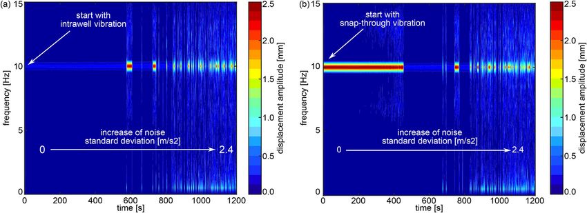
bration. This trend is opposite to that of system 1 and 2. The Fourier transforms of the simulated displacement responses for
system 3 across the time duration are presented in Fig. 9. The results in Fig. 9(a and b) show the broad range of spectral
behaviors as the standard deviation of noise increases from 0 to 2.4 m/s2. Between 9(a) and (b), the initial conditions are
selected to either induce intrawell or snap-through vibration for the simulation start when only harmonic base acceleration
occurs. In the time durations near 450e600 s, both simulations show small amplitude vibration that suggests an incapability
to sustain snap-through vibration. Yet, still further increase of noise standard deviation such as around 1200 s in Fig. 9 reveals
a snap-through-like behavior again. In contrast to the specific phenomena identified for the large asymmetrical system in
simulations and experiments, the analysis still indicates a similar snap-through dominant vibration as in systems 1 and 2.
In order to explain the discrepancy between analysis and simulation for greater system asymmetry, three additional cases
of asymmetry are considered. System 2 leads to a value for stiffness parameter k2 of 4 kN/m2. In the additional asymmetrical
systems, the parameter k2 is changed to 6 kN/m2, 8 kN/m2, or 10 kN/m2. Fig. 7 shows the potential energy shapes for the
asymmetrical energy harvesting systems. As shown in Fig. 7, the depth of the potential wells change as a result of the differing
asymmetry. With the increase of k2 , the difference between two potential wells depth increases.
For the case that snap-through vibration is frequently induced, the probability distribution function accurately employs
the factor of 1/2 for the two distribution functions shown in Eq. (24) so long as the system is symmetric so that the depths of
the potential wells are identical. Yet, with the introduction of asymmetry, it is not equally likely that the mean-square
displacement will adopt a zero mean value. Consequently, an accommodation is required to characterize amount by which
the probability distribution function changes. The Eq. (31) modifies the original distribution in Eq. (24) according to the
coefficients p1 and p2 which are the potential energies respectively associated with the stable equilibrium position x1 and x2 .
In this way, the cumulative contributions from the two distributions gðxrm jx1 ; sxg Þ and gðxrm jx2 ; sxg Þ, which are Gaussian
distributions with mean values x1 and x2 , account for the asymmetry on an energy basis.
Fig. 9. Short-time Fourier transform of simulated displacement response across the duration with the increase of noise standard deviation for system 3. Response
starts with (a) intrawell vibration and (b) snap-through vibration.W. Cai, R.L. Harne / Journal of Sound and Vibration 482 (2020) 115460 13
0.25
system 2
system 2 with k2=6[kN/m2]
system 2 with k2=8[kN/m2]
0.20
system 2 with k2=10[kN/m2]
probability density function
system 3
0.15
0.10
0.05
0.00
-6 -4 -2 0 2 4 6
nondimensional displacement
Fig. 10. Probability density functions for the asymmetrical energy harvesting systems.
p1 p2
f3 ðxrm Þ ¼ g xrm jx1 ; sxg þ g xrm jx2 ; sxg (31)
p1 þ p2 p1 þ p2
Using the expression in Eq. (31) considering that the radicand in Eq. (22b) is a unit valued constant, Fig. 10 presents the
probability density functions for the asymmetrical systems when subjected to non-dimensional noise standard deviation s ¼
1:5. The corresponding mean displacement values are numerically integrated through Eq. (31) for the system 2 cases shown
in Fig. 10. The mean displacement values are found to be 0.4951 mm for k2 ¼ 4 kN/m2, -0.7351 mm for k2 ¼ 6 kN/m2,
-0.8852 mm for k2 ¼ 8 kN/m2, and -1.167 mm for k2 ¼ 10 kN/m2. The dynamical responses for the systems characterized in
Fig. 10 are shown in Fig. 11. At noise standard deviation 2 m/s2, the mean displacement value from simulations in Fig. 11 are
around the mean displacement value calculated from the probability functions and listed above. This validates the energy-
weighted coefficients used in the probability density function for asymmetric systems, Eq. (31).
Based on the probability density plots in Fig. 10, for system 3 with large asymmetry there is a much greater possibility to
realize intrawell vibration with mean displacements closer to the negative valued equilibrium seen in Fig. 7. Since the increase
in asymmetry may increase the contrast between the weighted Gaussian distribution Eq. (23) and the accurate distribution in
Eq. (31) as in Figs. 2 and 10, the discrepancies in dynamical responses shown in Figs. 8 and 11 may also increase.
According to these investigations, when under the same excitation condition, vibration energy harvesting systems
exploiting nonlinearities yet subjected to ambient vibrations with harmonic and stochastic contributions are susceptible to
reduced performance if the nonlinearity is large enough to cause high asymmetry in the potential energy. For robust per-
formance and consistent DC power delivery, it is recommended to reduce asymmetry that may result from nonlinearities in
the implementation of energy harvesters in practical vibration environments.
5. Discussion on the dynamic responses
In Section 4, the dynamic responses are investigated using one value for the harmonic base acceleration component. As the
potential energy profiles vary with asymmetry such as in Fig. 7, the kinetic energy needed to overcome potential energy
barriers and realize snap-through vibration is changed. This indicates that the combination of harmonic and stochastic base
accelerations together crucially determine vibration of the energy harvesting system. This section investigates cases in which
the distinct dynamic behaviors transition as a result changes in the balance between harmonic and stochastic acceleration
components.
Fig. 12 presents the responses for the systems 1, 2, and 3. In Fig. 12, systems 1 and 2 are driven with a harmonic base
acceleration of 2.7 m/s2, while two cases of system 3 are studied using 5 m/s2 or 8 m/s2. Comparing the results in Figs. 4(a) and
12(a), with the increase of noise standard deviation s the mean displacement value for system 1 decreases to be a value
around zero, analogous to the unstable equilibrium position around which snap-through occurs. Yet, unlike the trend in
Fig. 4(c), for a stochastic base acceleration near 0.7 m/s2 in Fig. 12(b), the mean square voltage substantially drops. This is
similar to the trend shown in Fig. 8(c) for the asymmetric systems and indicates that an intrawell dominant vibration occurs.
Such vibration behavior is exemplified in Fig. 13(a) for noise standard deviation 1.6 m/s2. From Fig. 13(a), although the noise
may trigger jumps between the two equilibria, the regularity of generating snap-through vibration is low. A similar trend
occurs for system 2 in Fig. 12(a and b) for the smaller value of harmonic base acceleration 2.7 m/s2.
By contrast, for the harmonic base excitation of 5 m/s2, the dynamics of system 3 in Fig. 12 suggest a snap-through
dominant vibration, based on the larger mean square voltage values for most cases of additive noise base acceleration.14 W. Cai, R.L. Harne / Journal of Sound and Vibration 482 (2020) 115460
(a) 3.0 (b) 110
100
absolute mean displacement value [mm]
2.5 90
mean square voltage [V2]
80
2.0 simulation
analysis mean std 70
k2=4[kN/m2]
60
1.5 k2=6[kN/m2]
k2=8[kN/m2] 50
k2=10[kN/m2] 40
1.0
30
0.5 20
10
0.0 0
0.0 0.5 1.0 1.5 2.0 0.0 0.5 1.0 1.5 2.0
standard deviation of random excitation [m/s2] standard deviation of random excitation [m/s2]
Fig. 11. Analytical and numerical responses for four asymmetrical energy harvesting systems with harmonic amplitude 3.3 m/s2 and frequency 9 Hz. (a) Absolute
mean value of displacement amplitude. (b) Mean square voltage.
(a) 3.0 (b) 140
absolute mean displacement value [mm]
120
2.5
mean square voltage [V2]
100
2.0 simulation
analysis mean std
2
system 1: ah=2.7[m/s ] 80
2
system 2: ah=2.7[m/s ]
1.5
system 3: ah=5.0[m/s2]
60
system 3: ah=8.0[m/s2]
1.0
40
0.5
20
0.0 0
0.0 0.2 0.4 0.6 0.8 1.0 1.2 1.4 1.6 0.0 0.2 0.4 0.6 0.8 1.0 1.2 1.4 1.6
standard deviation of random excitation [m/s2] standard deviation of random excitation [m/s2]
Fig. 12. Analytical and numerical responses for system 1 and 2 at frequency 9 Hz and system 3 at 10 Hz. (a) Absolute mean value of displacement amplitude. (b)
Mean square voltage.
(a) 4 (b)
system 1: ah=2.7[m/s2]; σr=1.6[m/s2] 4 system 3: ah=5.0[m/s2]; σr=1.6[m/s2]
3
3
2
2
displacement [mm]
displacement [mm]
1 1
0 0
-1 -1
-2
-2
-3
-3
-4
-4
100 120 140 160 180 200 100 120 140 160 180 200
time [s] time [s]
Fig. 13. Transient displacements from simulation considering stochastic base acceleration of 1.6 m/s2 for (a) system 1 at harmonic excitation 2.7 m/s2 and (b)
system 3 at harmonic excitation 5 m/s2.
Fig. 13(b) shows a time series of the system 3 when driven by 5.0 m/s2 harmonic base acceleration and 1.6 m/s2 standard
deviation of stochastic base acceleration. Comparing the analytical and simulation results for the three systems in Figs. 4, 8
and 12, for increase of harmonic base excitation amplitude the discrepancy between simulation and analysis decreases. For
instance, for system 3 driven by harmonic base acceleration of 8 m/s2, the results of Fig. 12 suggest that snap-throughW. Cai, R.L. Harne / Journal of Sound and Vibration 482 (2020) 115460 15
vibration between the stable equilibria is frequently induced. In such case, the discrepancies between the simulation and
analysis are lessened.
One explanation for the changes in the discrepancy between analysis and simulation pertains to the influence of the
harmonic base acceleration on the effective probability density distribution functions determined by Eq. (24) [31]. With
increase in the harmonic excitation component, the possibility of triggering the snap-through vibration is increased. For
example, when the harmonic base acceleration for system 3 is 8 m/s2, snap-through vibration occurs even without presence
of stochastic base acceleration. In other words, once stochastic excitation is then introduced, the probability distribution
should be similar to that shown in Fig. 2(c) regardless of the standard deviation of the noise. In contrast, when the harmonic
base acceleration is too small to generate snap-through vibration, the probability density distribution should intuitively
appear like that represented in Fig. 2(a) or Fig. 10. In such latter case, only with increase of stochastic base acceleration should
the effective probability distribution function transition to a unimodal distribution. This suggests that for nonlinear energy
harvesting systems subjected to combined harmonic and stochastic base excitation, the weighted Gaussian distribution
implementation to lead to Eq. (25) results in better estimation of dynamical responses for greater amplitudes of harmonic
base acceleration because the response statistics are more comparable to those for a Gaussian distribution [49].
6. Conclusion
This research examines the dynamics of nonlinear energy harvesting systems under combined harmonic and stochastic
excitation to demonstrate the influences of asymmetry and relative balance of excitation components on the electrodynamic
responses and DC power delivery. An analytical approach based on the equivalent linearization method is established to
account for contributions to dynamics from harmonic and stochastic vibration inputs. A weighted Gaussian joint distribution
is adopted in the analytical model to improve the accuracy in predicting the statistical responses due to the stochastic
excitation. The discrepancies between simulations and analyses are scrutinized thorough study of the probability density
distributions. Combined with validation from simulations and experiments, the study reveals that with the increase of noise
intensity, the vibration becomes independent on initial conditions, and snap-through or intrawell dominant vibration may
occur. Through the investigations, the findings overall suggest that reducing asymmetry or increasing the harmonic excitation
component may trigger snap-through dominant vibration for moderate to high standard deviation of stochastic base ac-
celeration. The outcomes help identify robust energy harvesting system design approaches for consistent DC power delivery
when the platforms are subjected to realistic vibration environments.
Declaration of competing interest
The authors declare no conflicts of interest in this submission.
Acknowledgments
This research is supported by the National Science Foundation under Award No. 1661572. The authors are grateful to Mide
Technology for hardware support.
References
[1] M. Jia, A. Komeily, Y. Wang, R.S. Srinivasan, Adopting Internet of Things for the development of smart buildings: a review of enabling technologies and
applications, Autom. ConStruct. 101 (2019) 111e126.
[2] A. Darwish, A.E. Hassanien, M. Elhoseny, A.K. Sangaiah, K. Muhammad, The impact of the hybrid platform of internet of things and cloud computing on
healthcare systems: opportunities, challenges, and open problems, Journal of Ambient Intelligence and Humanized Computing (2017) 1e16.
[3] M. Díaz, C. Martín, B. Rubio, State-of-the-art, challenges, and open issues in the integration of Internet of things and cloud computing, J. Netw. Comput.
Appl. 67 (2016) 99e117.
[4] L. Reindl, Power Supply for Wireless Sensor Systems, 2018 [Online], http://www.sensornets.org/Documents/Previous_Invited_Speakers/2018/
SENSORNETS2018_Reindl.pdf.
[5] A. Hande, R. Bridgelall, B. Zoghi, Vibration energy harvesting for disaster asset monitoring using active RFID tags, Proc. IEEE 98 (9) (2010) 1620e1628.
[6] F. Cottone, H. Vocca, L. Gammaitoni, Nonlinear energy harvesting, Phys. Rev. Lett. 102 (8) (2009), 080601.
[7] A. Erturk, D.J. Inman, Broadband piezoelectric power generation on high-energy orbits of the bistable Duffing oscillator with electromechanical
coupling, J. Sound Vib. 330 (10) (2011) 2339e2353.
[8] M. Ferrari, V. Ferrari, M. Guizzetti, B. Ando , S. Baglio, C. Trigona, Improved energy harvesting from wideband vibrations by nonlinear piezoelectric
converters, Sensor Actuator Phys. 162 (2) (2010) 425e431.
[9] A. Erturk, J. Hoffmann, D.J. Inman, A piezomagnetoelastic structure for broadband vibration energy harvesting, Appl. Phys. Lett. 94 (25) (2009) 254102.
[10] T. Huguet, M. Lallart, A. Badel, Orbit jump in bistable energy harvesters through buckling level modification, Mech. Syst. Signal Process. 128 (2019)
202e215.
[11] J. Wang, W.H. Liao, Attaining the high-energy orbit of nonlinear energy harvesters by load perturbation, Energy Convers. Manag. 192 (2019) 30e36.
[12] Z. Zhou, W. Qin, W. Du, P. Zhu, Q. Liu, Improving energy harvesting from random excitation by nonlinear flexible bi-stable energy harvester with a
variable potential energy function, Mech. Syst. Signal Process. 115 (2019) 162e172.
[13] Q. Wang, N. Wu, Optimal design of a piezoelectric coupled beam for power harvesting, Smart Mater. Struct. 21 (8) (2012), 085013.
[14] R. Hosseini, M. Hamedi, Improvements in energy harvesting capabilities by using different shapes of piezoelectric bimorphs, J. Micromech. Microeng.
25 (12) (2015) 125008.
[15] B. Montazer, U. Sarma, Design and optimization of quadrilateral shaped PVDF cantilever for efficient conversion of energy from ambient vibration, IEEE
Sensor. J. 18 (10) (2018) 3977e3988.
[16] J.M. Dietl, E. Garcia, Beam shape optimization for power harvesting, J. Intell. Mater. Syst. Struct. 21 (6) (2010) 633e646.16 W. Cai, R.L. Harne / Journal of Sound and Vibration 482 (2020) 115460
[17] W. Cai, R.L. Harne, Vibration energy harvesters with optimized geometry, design, and nonlinearity for robust direct current power delivery, Smart
Mater. Struct. 28 (7) (2019), 075040.
[18] W. Cai, R.L. Harne, Optimized piezoelectric energy harvesters for performance robust operation in periodic vibration environments, in: Active and
Passive Smart Structures and Integrated Systems XII, 2019. Denver,Colorado.
[19] W. Liu, C. Zhao, A. Badel, F. Formosa, Q. Zhu, G. Hu, Compact self-powered synchronous energy extraction circuit design with enhanced performance,
Smart Mater. Struct. 27 (4) (2018), 047001.
[20] W. Cai, R.L. Harne, Electrical power management and optimization with nonlinear energy harvesting structures, J. Intell. Mater. Syst. Struct. 30 (2)
(2019) 213e227.
[21] E. Lefeuvre, A. Badel, C. Richard, D. Guyomar, Piezoelectric energy harvesting device optimization by synchronous electric charge extraction, J. Intell.
Mater. Syst. Struct. 16 (10) (2005) 865e876.
[22] E. Lefeuvre, A. Badel, A. Brenes, S. Seok, C.S. Yoo, Power and frequency bandwidth improvement of piezoelectric energy harvesting devices using
phase-shifted synchronous electric charge extraction interface circuit, J. Intell. Mater. Syst. Struct. 28 (20) (2017) 2988e2995.
[23] Q. He, M.F. Daqaq, Influence of potential function asymmetries on the performance of nonlinear energy harvesters under white noise, J. Sound Vib. 333
(2014) 3479e3489.
[24] W. Wang, J. Cao, C.R. Bowen, D.J. Inman, J. Lin, Performance enhancement of nonlinear asymmetric bistable energy harvesting from harmonic, random
and human motion excitations, Appl. Phys. Lett. 112 (21) (2018) 213903.
[25] C. Zhang, R.L. Harne, B. Li, K.W. Wang, Statistical quantification of DC power generated by bistable piezoelectric energy harvesters when driven by
random excitations, J. Sound Vib. 442 (2019) 770e786.
[26] R.L. Harne, M. Thota, K.W. Wang, Concise and high-fidelity predictive criteria for maximizing performance and robustness of bistable energy har-
vesters, Appl. Phys. Lett. 102 (5) (2013), 053903.
[27] Y. Chen, M.Q. Feng, C.A. Tan, Modeling of traffic excitation for system identification of bridge structures, Comput. Aided Civ. Infrastruct. Eng. 21 (1)
(2006) 57e66.
[28] J.D. Turner, A.J. Pretlove, A study of the spectrum of traffic-induced bridge vibration, J. Sound Vib. 122 (1) (1988) 31e42.
[29] N.D. Anh, N.N. Hieu, The Duffing oscillator under combined periodic and random excitations, Probabilist. Eng. Mech. 30 (2012) 27e36.
[30] R.N. Iyengar, A nonlinear system under combined periodic and random excitation, J. Stat. Phys. 44 (5e6) (1986) 907e920.
[31] Z.L. Huang, W.Q. Zhu, Y. Suzuki, Stochastic averaging of strongly non-linear oscillators under combined harmonic and white-noise excitations, J. Sound
Vib. 238 (2) (2000) 233e256.
[32] Y.J. Wu, W.Q. Zhu, Stochastic averaging of strongly nonlinear oscillators under combined harmonic and wide-band noise excitations, J. Vib. Acoust. 130
(5) (2008), 051004.
[33] A.R. Bulsara, K. Lindenberg, K.E. Shuler, Spectral analysis of a nonlinear oscillator driven by random and periodic forces. I. Linearized theory, J. Stat.
Phys. 27 (4) (1982) 787e808.
[34] H. Kim, W.C. Tai, J. Parker, L. Zuo, Self-tuning stochastic resonance energy harvesting for rotating systems under modulated noise and its application to
smart tires, Mech. Syst. Signal Process. 122 (2019) 769e785.
[35] Q. Dai, R.L. Harne, Investigation of direct current power delivery from nonlinear vibration energy harvesters under combined harmonic and stochastic
excitations, J. Intell. Mater. Syst. Struct. 29 (4) (2018) 514e529.
[36] S. Zhou, L. Zuo, Nonlinear dynamic analysis of asymmetric tristable energy harvesters for enhanced energy harvesting, Commun. Nonlinear Sci.
Numer. Simulat. 61 (2018) 271e284.
[37] S. Fang, X. Fu, W.H. Liao, Asymmetric plucking bistable energy harvester: modeling and experimental validation, J. Sound Vib. 459 (2019) 114852.
[38] S.F. Ali, S. Adhikari, M.I. Friswell, S. Narayanan, The analysis of piezomagnetoelastic energy harvesters under broadband random excitations, J. Appl.
Phys. 109 (7) (2011), 074904.
[39] J. Liang, W.H. Liao, Impedance modeling and analysis for piezoelectric energy harvesting systems, IEEE ASME Trans. Mechatron. 17 (6) (2011)
1145e1157.
[40] Y.C. Shu, I.C. Lien, Analysis of power output for piezoelectric energy harvesting systems, Smart Mater. Struct. 15 (6) (2006) 1499.
[41] W.A. Jiang, L.Q. Chen, Stochastic averaging based on generalized harmonic functions for energy harvesting systems, J. Sound Vib. 377 (2016) 264e283.
[42] Z. Xu, Y.K. Cheung, Averaging method using generalized harmonic functions for strongly non-linear oscillators, J. Sound Vib. 174 (4) (1994) 563e576.
[43] H. Makarem, H.N. Pishkenari, G.R. Vossoughi, A modified Gaussian moment closure method for nonlinear stochastic differential equations, Nonlinear
Dynam. 89 (4) (2017) 2609e2620.
[44] H.T. Zhu, S.S. Guo, Periodic response of a Duffing oscillator under combined harmonic and random excitations, J. Vib. Acoust. 137 (4) (2015).
[45] A. Erturk, D.J. Inman, Piezoelectric Energy Harvesting, John Wiley & Sons, Chichester, 2011.
[46] Q. Dai, R.L. Harne, Charging power optimization for nonlinear vibration energy harvesting systems subjected to arbitrary, persistent base excitations,
Smart Mater. Struct. 27 (1) (2017), 015011.
[47] J.A. Hansen, C. Penland, Efficient approximate techniques for integrating stochastic differential equations, Mon. Weather Rev. 134 (10) (2006)
3006e3014.
[48] R.L. Harne, K.W. Wang, A review of the recent research on vibration energy harvesting via bistable systems, Smart Mater. Struct. 22 (2) (2013), 023001.
[49] M. Dykman, K. Lindenberg, Fluctuations in nonlinear systems driven by colored noise, in: G.H. Weiss (Ed.), Contemporary Problems in Statistical
Physics, SIAM, Philadelphia, 1994 ch. 2.You can also read