Urban Microclimate and Its Impact on Building Performance: A Case Study of San Francisco
←
→
Page content transcription
If your browser does not render page correctly, please read the page content below
1    Urban Microclimate and Its Impact on Building
2    Performance: A Case Study of San Francisco
 3    Abstract: Urban microclimate exerts an increasing influence on urban buildings, energy,
 4    and sustainability. This study uses 10-year measured hourly weather data at 27 sites in San
 5    Francisco, California, to (1) analyze and visualize the urban microclimate patterns and
 6    urban heat island effect; (2) simulate annual energy use and peak electricity demand of
 7    typical large office buildings and large hotels to investigate the influence of urban
 8    microclimate on building performance; (3) simulate indoor air temperature of a single-
 9    family house without air-conditioning during the record three-day heatwave of 2017, to
10    quantify the divergence of climate resilience due to urban microclimate effect. Results
11    show significant microclimate effects in San Francisco with up to 11℃ outdoor air
12    temperature difference between the coastal and downtown areas on September 1, 2017,
13    during the record three-day heatwave. The simulated energy results of the prototype large
14    office and large hotel buildings using the 2017 weather data show over 100% difference in
15    annual heating energy use and 65% difference in annual cooling energy use across
16    different stations; as well as up to 30% difference in peak cooling electricity demand. The
17    impacts on annual site or source energy use are minimal (less than 5%) as cooling and
18    heating in a mild climate are a relatively small portion of overall building energy use in
19    San Francisco. Results also show the microclimate effects influence indoor air temperature
20    of unconditioned homes by up to 5℃. Newer buildings and homes are much less affected
21    by microclimate effects due to more stringent performance requirements of the building
22    envelope and energy systems. These findings inform that San Francisco microclimate
23    variations should be considered in urban energy planning, building energy codes and
24    standards, as well as heat resilience policymaking.

25    Keywords: Urban microclimate; CityBES; building energy use; building performance;
26    building simulation; climate resilience
27

28   1. Introduction
29        A microclimate can be defined as any area where the climate differs from its
30   surrounding area [1]. Urban microclimate refers to the local climate effects in cities and
31   urban areas, which observe a higher heterogeneity than their surrounding rural areas [2].
32   The features of an urban microclimate include variations in outdoor air temperature, surface
33   temperature, humidity, wind speed, and wind direction [3]. Several human-induced factors
34   can cause urban microclimates. Building and construction materials can affect the albedo,
35   thermal conductivity, and different heat capacity of urban surfaces, and therefore impact the
36   amount of reflected energy [4]. In the meantime, less evapotranspiration from plants, fewer
37   water surfaces, and less irrigation in typical urban areas can lead to lower latent heat
38   exchange with the outdoor environment. Urban morphology, including building densities
39   and heights, can affect the wind patterns [5], shading patterns [6], and create the thermal
40   trappings between dense buildings (e.g., the urban canyon effect) [7]. Moreover,
41   anthropogenic heat (from vehicles, buildings, industry, and human metabolism, etc.)
42   dispersed into the urban environment is one of the most important causes of the urban heat
43   island (UHI) effect [8]. Researchers have studied the spatiotemporal variations of the UHI
44   due to the changes in land-use/land-cover, urban sprawling, and population shifts [9], and
45   found the spatial distribution and seasonal patterns of urban thermal patterns can be diverse
46   across the studied urban area [10].
47        Local weather conditions determine the heat and mass flow between buildings and their
48   environment through (1) conductive and convective heat flux at the urban surfaces, (2) solar
49   and long-wave radiation exchange, and (3) sensible and latent heat transfer through
50   ventilation and infiltration [11]. Hence, urban climate and microclimate can strongly
51   influence building energy use, demand, and building thermal resilience. Toparlar et al.
52   performed building energy simulations based on different microclimate conditions with a
53   set of prototype buildings in July 2013 in Antwerp, Belgium [2]. The results demonstrated
54   that average air temperatures at the urban sites away from the park was 0.9 °C higher than
55   the area close to the park, and the residential buildings near the park had 13.9% less cooling
56   demand than those away from the same park. Bourikas also demonstrated that microclimate
57   plays an essential role in building heating and cooling loads [12]. The study used the actual
58   measurements of air temperature and relative humidity at 26 sites within a 250-meter radius
59   in Hangzhou, China, and the results showed that up to 20% differences were observed in
60   the heating and cooling loads computed with/without microclimate considerations. In recent
61   years, building resilience to urban microclimate variations has also become a significant
62   topic. Chokhachian et al. presented methods to evaluate urban resilience at a micro-scale.
63   The study used mobile micro-meteorological sensors to measure wind speed, air
64   temperature, humidity, globe temperature, and solar radiation, and calculated the universal
65   thermal comfort Index (UTCI) score to access outdoor comfort under heat events [13].
66   Katal et al. also applied the urban microclimate simulation tool, City Fast Fluid Dynamics
67   (CityFFD), to model a snowstorm event with more than 1500 buildings in Montreal,
68   Canada, investigating their resilience against the three-day power outage due to the storm
69   [14].
70        Various approaches have been employed in the past decades to quantify the urban
71   microclimate, including field data measurement and collection, remote sensing and GIS-
72   based assessment, and computational simulation and modeling [15]. Historically, most
73   urban microclimate studies were conducted by collecting measurement data from different
74   parts of an urban area [16]–[20]. For example, Pioppi et al. carried out a cluster analysis
75   with data-driven identification of urban microclimate peculiarities to its morphology, and
76   the measurements in the dense district show a non-negligible dependency on the urban land
77   cover both in winter and in summer [21]. Measurements in urban areas can face some
78   challenges, such as the problem of data quality issues, spatial representativeness, and the
79   lack of sufficient weather parameters [22]. However, in recent studies, some of these
80   challenges can be overcome with the applications of emerging technologies, such as low-
81   cost sensor networks distributed vastly in urban areas [23]. Urban microclimate can also be
82   investigated with modeling and simulation approaches [24]–[30]. Computational Fluid
83   Dynamics (CFD) is also frequently used to assess and predict urban microclimate in a finer
84   spatial resolution [14], [31]. For example, Javanroodi and Nik use CFD simulation
85   generated weather data based on mesoscale metrological models to study the overall energy
86   performance of buildings. Considering the fluctuations of air pressure, relative humidity,
87   and heat flux, the average and peak outside surface temperature showed over 67% and 7%
88   higher magnitude, respectively, compared to typical weather. Simulation methods allow
89   investigating urban microclimate effects under a variety of urban morphology and design
90   scenarios, and can generate more targeted weather parameters with higher fidelity [32].
91        San Francisco is a coastal city in Northern California, USA. It has a mild climate
92   (climate zone 3C) and an area of 121.4 km2. Even though the city is not large
93   geographically, its local weather can vary significantly across the city. During the record
94   three-day heatwave event in September 2017, there were six heat-related deaths in the San
 95   Francisco Bay Area, and a large difference in outdoor air temperature of up to 11℃ was
 96   observed between the coastal and downtown area of San Francisco. Such microclimate
 97   variations have substantial implications on building energy demand and outdoor thermal
 98   environment. In this study, we analyzed 10-year hourly weather data measured at 27
 99   weather stations across San Francisco, and visualized the results using microclimate maps
100   with the CityBES tool to reveal the spatial patterns and temporal trends (Section 2). We
101   also use building energy modeling to quantify the urban microclimate impact on building
102   energy demand and thermal resilience using local weather data at 14 sites (Section 3). Here,
103   the impact refers to the same building in different locations of San Francisco having
104   different energy uses and peak demands due to local microclimate conditions. Section 4
105   describes implications of the results, limitations of this study and potential future research.
106   Conclusions are drawn in Section 5.

107   2. San Francisco Microclimate
108        We developed a web-based map interface to visualize the spatial variation and
109   temporal trends of a city’s local climate, and use San Francisco as a case study to
110   demonstrate the features. It is part of the CityBES, a free-to-use open data and computing
111   platform for city buildings, energy, and sustainability [33]. CityBES, an urban building
112   energy modeling tool [34], [35], simulates the energy performance of a city’s building
113   stock [36], from a small group of buildings in an urban district to all buildings in a city.
114   CityBES builds upon the Commercial Building Energy Saver Toolkit [37], which provides
115   retrofit analysis of individual commercial and residential buildings using a comprehensive
116   library of more than 100 energy technologies and control strategies. CityBES also provides
117   a quick assessment of district energy systems using EnergyPlus simulations. CityBES uses
118   CityGML and GeoJSON as the data schema to represent the urban building stock [38]. It
119   provides 3D visualization of the building shapes and an array of performance metrics for
120   whole-building energy use and end uses, peak electricity demand, utility costs, GHG
121   emissions, energy savings, and retrofit economics.

122   2.1. Data Source and Data Cleaning
123        San Francisco weather data— hourly weather data of 2008 to 2017 were acquired
124   from White Box Technologies [39]. The data set consists of 149 weather files in
125   EnergyPlus epw format, each with a one-year duration, containing 22 weather variables.
126   The format and detailed variable descriptions follow the EnergyPlus weather data definition
127   [40]. Among the files we received, seven of them have non-matching weather station IDs in
128   the weather file, and in the file name. This makes it difficult to locate the associated stations
129   for those files. Mis-placing weather station data will impair the accuracy of the spatial
130   interpolation. Thus we removed them from the data set. The second cleaning step involves
131   dropping measurements with invalid data ranges. In this step, we removed three records
132   with negative relative humidity values. After cleaning, we selected four variables to
133   visualize in the interface: dry bulb temperature (⁰F), relative humidity (%), global
134   horizontal radiation (Wh/m2), and wind speed (m/s). There are 27 weather stations in the
135   cleaned data set. Figure 1 shows the location and start and end year of each weather station.
136   Table 1 lists the summary statistics of the four variables across the 10-year period at 27
137   stations. Overall, San Francisco has a mild climate with limited seasonal differences in
138   average ambient air temperature and relative humidity. On the other hand, the distributions
139   of many weather variables are heavily tailed with many extremely high or low records,
140   especially the wind speed in winter months and the dry bulb temperature in summer
141   months.

142      Figure 1. Weather Stations in San Francisco

143                     Table 1. Summary Statistics of San Francisco Hourly Weather Data at 27 sites.

                                                   Mi      Media       Mea                 Skewnes      Kurtos
                            Variables               n      n            n        Max          s           is
                                                   26.
                          DryBulb (F)               1       55.8        56.4     107.6         0.8       4.9
                          GloHorzRad                                    200.     1142.
         Overall           (Wh/m2)                 0.0      12.0         3         0           1.3       3.4
                                                   0.0
                       RelHum (percent)             *       84.0        78.4     100.0         -1.1      3.4
                        WindSpd (m/s)              0.0       0.5         1.2      19.6          2.1      9.4
                                                   32.
                          DryBulb (F)               4       52.7        53.2      80.2         0.5       3.3
                          GloHorzRad                                    142.
         Februar
                           (Wh/m2)                 0.0       0.0         0       870.0         1.3       3.3
            y
                                                   7.0
                       RelHum (percent)             *       82.0        77.5     100.0         -0.9       3.2
                        WindSpd (m/s)              0.0       0.3         1.0      19.1          2.7      13.6
         August                                    34.
                         DryBulb (F)                9       59.0        60.0     100.0         1.3       6.1
                         GloHorzRad                                     241.     1055.
                           (Wh/m2)                 0.0      70.0         0         0            1.0      2.6
                       RelHum (percent)            0.0      90.0        84.8     100.0         -1.6      5.3
                                                    *
WindSpd (m/s)        0.0     1.2      1.7     17.0       1.2        4.1
144    *The very low relative humidity can be due to data quality issues of those data points.
145
146        San Francisco geographical boundary—The shapefile of the geographical boundary of
147   San Francisco is retrieved from DataSF [41].
148        In addition to the four direct measurements, the interface also displays four derived
149   weather metrics: heating degree-day (HDD), cooling degree-day (CDD), heat index (HI),
150   and urban heat island index (UHII). HDD and CDD could inform urban planners and
151   policymakers about the potential heating and cooling loads at various locations and at
152   different times of the year. Heat index and UHII could assist policy analysis of adaptation
153   strategies to short-term heatwaves and long-term climate change. The calculations of the
154   derived metrics are described as follows.

155   2.1.1 HDD and CDD
156       Degree-days are often used for a rough estimation of the heating or cooling load.
157   Degree-days for a certain period P (e.g., a month or a year) are computed as the
158   accumulated difference between the mean daily temperature and some base temperature
159   (Equation 1 and 2). Here we use 65⁰F as the base temperature for heating degree day and
160   50⁰F for cooling degree day, consistent with the practice of ASHRAE handbooks [42].
                                        HDD P= ∑ max (0 , 65−T i,mean )                                (1)
                                                 i∈P

                                        CDD P= ∑ max (0 ,T i,mean−50 )                                 (2)
                                                 i∈P

161       T i,mean is the average of the daily max and the daily min temperature of day i in the
162   period P .

163   2.1.2 Heat Index (HI)
164        This metric reflects the hotness considering both temperature and relative humidity.
165   Adding humidity to the picture is essential, as the ambient moisture could affect the
166   evaporative cooling of the human body, which then influences how a certain temperature
167   feels like to the body. High HI could lead to various adverse health consequences, including
168   heat exhaustion or heat stroke [43]. The calculation follows the NOAA method [44]. First,
169   a simplified formula following Steadman's result is applied. This formula only has first-
170   order temperature and relative humidity terms. For high HI cases (higher than 80), the
171   Rothfusz formula with higher-order temperature and RH terms is used. This formula also
172   considers further adjustments for low RH and hot and humid cases.

173   2.1.3 Urban Heat Island Index (UHII)
174        Taha and Freed developed a UHII metric [45] as is shown in Equation 3, where the
175   UHII is calculated for each census tract as the accumulated hourly temperature difference
176   between the urban and the non-urban areas within the census tract. T c , h , urban is the
177   temperature for urban areas in census tract c at timestamp h . T c , h , non-urban is the temperature
178   for non-urban areas in census tract c at timestamp h . h ranges in the summer of 2013 and
179   2006.
                                         UHII= ∑ UHIIc , h= ∑ ¿ ¿ ¿)                                   (3)
                                                 h∈D             h∈D

180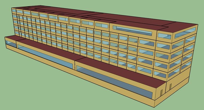
181 One issue of this definition is that the inner term UHIIc , h is un-defined for geographical
182 units with urban-only or non-urban-only land uses. We changed the non-urban reference
183 temperature from specific to each geographical unit T c , h , non-urban to the average across the
184 region T h ,non-urban =mea nc (T c , h , non-urban ). This could make UHIIc , h definable for the urban-
185 only geographical units. We also added an indicator l [ withUrban ( c ) ] that checks whether a
186 geographical unit contains some portion of urban land use. This could cover the
187 geographical units with only non-urban land uses.
UHIIc , h=l [ withUrban ( c ) ] ( T c ,h ,urban −min (T c ,h ,urban ,T h , non-urban )) (4)
188 Comparing with Taha and Freed UHII, the metric used in this study produces the same
189 aggregated results for UHII= ∑ UHI I c ,h when every geographical unit (for example,
h∈D
190 census tract) in the analysis has some portion of urban area and non-urban area. It also
191 defines UHIIc , h for geographical units with homogeneous urban or non-urban land uses.
192 This allows the metric to be applied to a finer geographical resolution, which is more likely
193 to have single land use within each geographical unit. We applied the modified UHII metric
194 to 30m x 30m gridded cells, and each cell c represents a 30m x 30m square region in San
195 Francisco.
196 We used the land use data to classify whether a cell on the map is
197 urban or non-urban. The land use data of San Francisco is a subset of
198 the 2011 National Land Cover Database (NLCD) raster file [46], retrieved
199 with the R package, FedData [47]. We label the “developed” land use
200 type (category 21 to 24 in NLCD) as an urban area, and the rest as a
201 non-urban area (Figure 2(a)).
(a) (b)
202 Figure 2. (a) Land use pattern from NLCD; (b) urban heat island index for April 2008
203 2.2. Interface Design
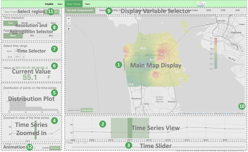
204 The map interface (Figure 3) displays the space-time patterns of various weather
205 metrics in the study region, with a 2D map view, a time slider, and an animation view
206 navigating through different snapshots of the map view, and some data summary charts.
207 Users can toggle the display of various weather metrics using the variable selector
208 (component 9). The spatial heterogeneity of each weather metric is presented as a heat map
209 overlaid on top of the regional map. The heat map of each weather variable is generated for
210 each time stamp with an inverse distance weighted spatial interpolation of measurements at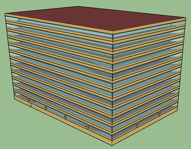
211   each weather station. The value of a weather variable at each location and each time stamp
212   is computed as a weighted average of values of all available weather stations at that time
213   stamp. The weight of each weather station is the reciprocal of the squared distance between
214   the target location and the weather station. This spatial interpolation is computed with the R
215   package, gstat [48]. Exact measurements at each weather station are shown as white labels
216   on the map. Users can navigate through different time stamps with a time slider at the
217   bottom of the interface.

                                                                (a)

                                                                (b)
218       Figure 3. (a) Components of the Interface; (b) a screenshot of the interface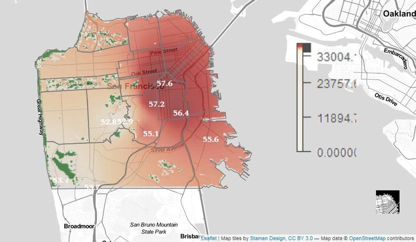
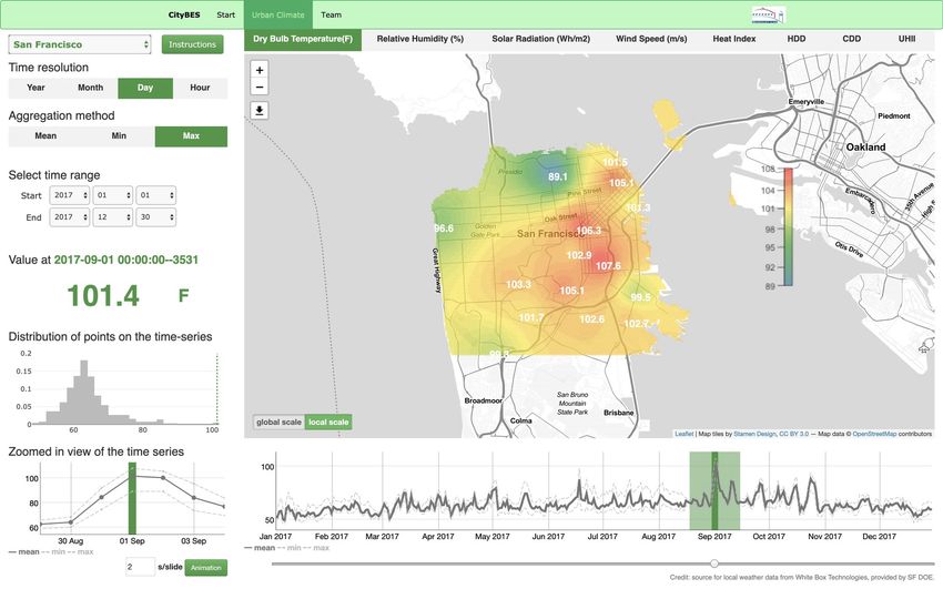
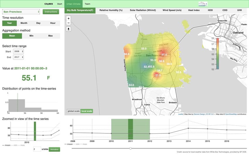
219        The temporal trend is shown as time-series plots (components 2 and 4). The plot below
220   the map window shows the spatial-temporal aggregation (the solid line) and the spatial
221   extremes (the min and max of the color-coded values displayed on the map, shown with
222   two dashed lines) of the temporal aggregation, and the plot at the bottom left corner is a
223   zoomed-in view of the time series plot at the current time stamp. A histogram to the left of
224   the map (component 5) shows the distribution of the spatial-temporal aggregation for the
225   displayed period, with the value of the current time step marked as a vertical dashed line.
226   The animation button (component 12) allows an automatic slide show of the visualization at
227   a speed set by the user, to display the changes of the selected microclimate variable over
228   time.
229        Weather variables are anticipated to have strong seasonality at various temporal scales,
230   thus we provided several temporal resolutions and temporal aggregation options
231   (component 8). For example, when the “year” resolution and the “mean” aggregation
232   method are chosen, weather station data are aggregated to annual averages. Then a heat
233   map is generated for each year with spatial interpolation of the annual average weather
234   station data. The scale of the heat map can be switched between “global” and “local” by the
235   toggle at the bottom left corner of the map, where the global scale uses the statistics of all
236   the historical data aggregated by the selected time resolution and aggregation method, and
237   the local scale uses the statistics of the current time stamp.
238        Apart from San Francisco, we also acquired historical weather data of Sydney,
239   Australia from the University of Sydney to visualize. Several other cities are under
240   development as well. Users can select the region of interest through the dropdown list at the
241   upper left corner (component 11).

242   2.3. Implementation
243        R is used for data cleaning, processing, image and data file (CSV or JSON) generation.
244   The heat maps are png images generated using the R raster package [49], gstat package
245   [48], and sf package [50]. The interface is written in HTML and JavaScript. We use Leaflet
246   [51] to create the map view and load the heat map image onto the regional map. The time-
247   series plots are created with dygraphs [52]. The histogram is produced with Plotly [53]. The
248   animation feature is implemented with JavaScript.

249   2.4. Example use cases
250       The visualization tool reveals some interesting patterns in the weather data. We present
251   three use cases as examples:
252   1. With the daily or hourly view, users could identify certain historical weather events.
253        For instance, in the 2017 daily dry-bulb temperature display (Figure 4), we could
254        observe the timing (September 1) and the magnitude (101.4⁰F) of the heatwave from
255        the time-series plot, and the current-value label (component 6). The distribution plot
256        further demonstrated that the temperature at the current time stamp is at the right end
257        of the distribution.
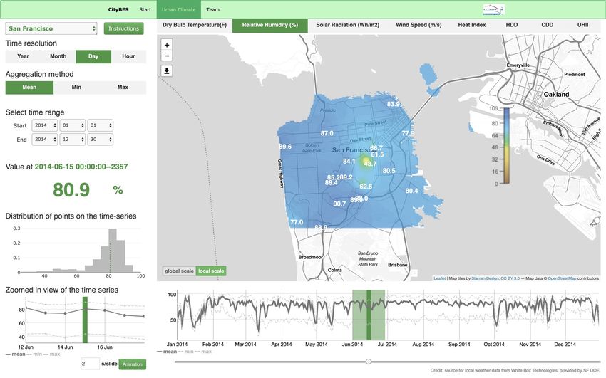
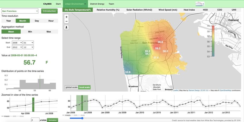
258        Figure 4. Identification and illustration of the historical heatwave on September 1, 2017 in San Francisco.

259   2.   With the monthly views, users could spot the seasonality of certain variables. For
260        example, we could observe strong seasonal patterns in temperature, solar radiation, and
261        wind speed, while relative humidity is relatively stable – not seasonal. Figure 5 shows
262        the average monthly ambient air temperature from 2008 to 2012, with a seasonal
263        pattern shown in the bottom time-series plot.

264
265        Figure 5. The monthly view shows the seasonal pattern of average monthly ambient air temperature.

266   3.   Using the time-series plot (component 2), users could identify the overall level of
267        spatial heterogeneity of a variable (the distance between the two dashed lines in the
268        bottom-right sub-figure showing the mean, min, and max of the displayed variable,
269        relative humidity in this case, in Figure 6). With the map view, the user could locate
270        the spatial extreme positions. For example, in the daily mean relative humidity view,
271        we notice substantial spatial variations where the maximum (90.7%) is over twice the
272        minimum (43.7%). The map view (Figure 6) shows the highest values are close to the
273        coastal area, and the lowest values appear in inland regions.
274

275        Figure 6. Spatial heterogeneity of ambient air relative humidity

276   3. Microclimate impact on building performance

277   3.1. Impact on building energy performance
278        A simulation study was performed to evaluate the impact of microclimate on building
279   energy use. The San Francisco weather data in 2017 at selected 14 stations were applied to
280   four DOE prototype building models [54], covering two building types (the large office and
281   the large hotel, as shown in Figure 7) and two vintages (2004 and 2013). The selected 14
282   stations, based on data quality, are R48, R49, R73, R79, R100, R107, R128, R161, R169,
283   R327, R348, R435, R887, R957, whose locations can be found in Figure 1. Table 2 lists the
284   geometry and HVAC characteristics of the two prototype buildings. Table 3 lists the
285   envelope properties of the two vintages, based on ASHRAE standards requirements.
286        EnergyPlus is used as the building performance simulation tool in this study to
287   calculate the annual energy use and peak demand of the four building models using the
288   weather files at the 14 weather stations. EnergyPlus is an open-source program that models
289   heating, ventilation, cooling, lighting, water use, renewable energy generation, and other
290   building energy flows [55] and is the flagship building simulation engine supported by the
291   United States Department of Energy (USDOE).
(a)                                                           (b)
292       Figure 7. 3D geometry of the prototype building models: (a) Large Office; (b) Large Hotel

293                     Table 2. Basic characteristics of the prototype large office and large hotel models

                                                   Large Office                                       Large Hotel
         Number of                                     12                                                 6
        floors above
           ground
         Number of                                         1                                                   1
       basement floors
       Total floor area                                46,320                                             11,350
            [m2]
        Window-to-                                        40                                                  30.2
        wall ratio (%)
        Heating type                        Gas-fired boilers                                      Gas-fired boilers
        Cooling type           Two water-cooled centrifugal chillers for                          Air-cooled chillers
                              most spaces. Water-source DX cooling coil
                                 with fluid cooler for data center in the
                                basement and IT closets in other floors;
        Distribution          VAV with hot-water reheat coils except non-                       Public spaces: VAV
        and terminal           datacenter portion of the basement and IT                        with hot water reheat
           units                 closets that are served by CAV units.                                 coils;
                                                                                                    Guest rooms:
                                                                                                dedicated outside air
                                                                                                 system + four-pipe
                                                                                                   fan-coil units.

294                                  Table 3. Envelope properties of vintage 2004 and 2013

                                                                                  2004         2013 [57]
                                                                                   [56]
                             Wall U-factor [W/m2-K]                               0.857           0.701
                             Roof U-factor [W/m2-K]                               0.357           0.220
                           Window U-factor [W/m2-K]                                6.93            3.12
                         Window Solar heat gain coefficient                        0.34            0.25
                                    (SHGC)

295       Figures 8-11 illustrate the box-whisker plots, which indicate the distribution of several
296   energy performance indices on the four prototype models, including the annual site and
297 source energy, annual cooling energy use (electricity), annual heating energy use (natural 298 gas), peak electricity & natural gas use. Key findings are summarized as follows: 299 (1) The impact of microclimate on the energy use of the HVAC systems is significant. 300 Using different microclimate data can lead to as much as over 100% difference in annual 301 heating energy use and 65% difference in annual cooling energy use. 302 (2) The impact of microclimate on the total annual site or source energy is much 303 smaller. This is because (1) microclimate only affects HVAC energy use, which accounts 304 for 20~25% of the total energy use in the large office, and 40~50% in the large hotel; in this 305 case, the relative impact on the total energy use is reduced. (2) the impacts on heating 306 demand and cooling demand compensate each other. For example, when the cooling 307 demand is increased under warmer weather, the heating demand is decreased, so the overall 308 impact is reduced. 309 (3) The impact of microclimate on building peak cooling and heating demand is 310 significant, as much as a 30% difference in peak cooling electricity demand and over 100% 311 difference in peak natural gas demand. This is critical from the supply-side perspective, as 312 it will directly affect the required utility generation capacity. The impact on the building 313 peak demand is a bit less than the peak HVAC demand because of other end uses (e.g., 314 lighting and plug loads). 315 (4) The impact of microclimate on energy performance varies with building types and 316 vintages. Cooling and heating loads mainly consist of (1) heat gains through the envelope, 317 mechanical ventilation, and infiltration, which microclimate has an impact on, and (2) heat 318 gains from other sources, such as occupant, lighting and plug loads, which do not change 319 with climate. The variation of the absolute values of energy performance is purely affected 320 by the former heat gains. On the other hand, the percentage difference is affected by the 321 proportion of former heat gains in the total load and the baseline level. All the above factors 322 vary with building types and vintages, resulting in different levels of microclimate impact 323 on building energy performance. 324 In summary, microclimate data are recommended for use in estimating the total 325 building energy consumption, especially considering the needs of a more accurate 326 estimation of the cooling and heating energy use, and more importantly, the peak demand, 327 from the perspective of the utility supply side.
328   Figure 8. Box-whisker plot of energy performance index for the large hotel of the 2004 vintage.

329   Figure 9. Box-whisker plot of energy performance index for the large hotel of the 2013 vintage.

330   Figure 10. Box-whisker plot of energy performance index for the large office of the 2004 vintage.
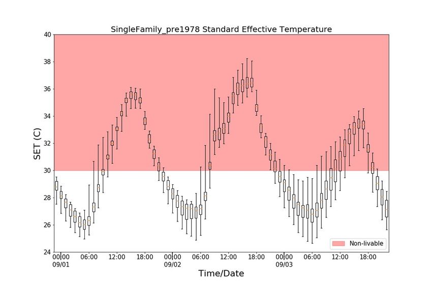
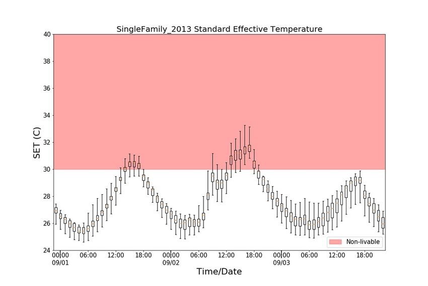
331        Figure 11. Box-whisker plot of energy performance index for the large office of the 2013 vintage.

332   3.2. Impact on indoor air temperature of unconditioned residential buildings
333       In San Francisco, it is very common that residential buildings are not equipped with air
334   conditioning systems due to the mild climate. Microclimate affects the indoor environment
335   of such unconditioned buildings, especially under extreme weather conditions. A
336   simulation study was conducted to investigate the impact of microclimate on indoor air
337   temperature of unconditioned residential buildings during heat waves.
338        The 2017 3-day heatwave was selected for this study, during which San Francisco
339   smashed all-time record high temperature and hit 106 degrees in the downtown area on
340   September 1, 2017 [58]. We adopt the one-story single-family prototype building as the
341   baseline model, which is from the Alternative Calculation Method Approval Manual for
342   California building energy efficiency standards Title 24 [59]. As shown in Figure 12, The
343   building has pitched roofs, an unconditioned attic under the roof, and an unconditioned
344   ground-level garage attached to the living zone. All the living area is modeled as a single
345   conditioned thermal zone. Two vintages, pre1978 and 2013, are simulated to represent old
346   and new constructions. The envelope properties and internal loads are derived from Title 24
347   minimum efficiency requirements [59], [60].
348 Figure 12. 3D geometry of the one-story single-family prototype building defined in the Title 24 ACM. 349 Figures 13 and 14 illustrate the hourly variations of outdoor air temperature and indoor 350 air temperature at all 14 weather stations during the three-day heatwave period. While the 351 outdoor air temperature differs as much as 11C among different locations during peak 352 hours, the indoor air temperature differ by a maximum of 5C. Recently built houses have 353 better envelope performance and lower internal heat gains due to more stringent code 354 requirements. As a result, the peak indoor air temperature and the difference of indoor air 355 temperature across the local 14 stations get reduced. 356 Standard effective temperature (SET) is a temperature metric that factors in relative 357 humidity, mean radiant temperature, air velocity, and anticipated activity rate and clothing 358 level of the occupants. SET is adopted to evaluate passive survivability by the U.S. Green 359 Building Council’s Leadership in Energy and Environmental Design (LEED) green 360 building program. The “Livable Temperatures” are defined as SET between 12.2°C and 361 30°C. The SET-hours is an accumulated metric to measure thermal safety based on the 362 indoor SET. It weights each hour when the indoor SET exceeds a certain threshold by the 363 number of degrees Celsius by which it surpasses that threshold. In this study, we adopt the 364 upper SET limit of “Livable Temperatures”, i.e., 30°C, as the threshold for calculating 365 SET-hours. Figures 15 and 16 illustrate the hourly variations of indoor SET and the 366 variation of accumulated SET-hours at all 14 weather stations. Among different 367 microclimates, the SET could differ by as much as 3C, and the highest SET-hours could be 368 twice the lowest SET-hours for the home built before 1978. Similar to the trend of indoor 369 air temperature, the SET-hours, peak SET, and the hourly variation range of SET all get 370 shrunk as the building performance gets better. 371 Figure 13. Hourly distribution of outdoor air temperature (September 2017) at all 14 weather stations.
(a) (b)
372 Figure 14. Hourly distribution of indoor air temperature in single-family homes at all 14 weather stations: (a)
373 Pre 1978; (b) 2013
(a) (b)
374 Figure 15. Hourly distribution of indoor standard effective temperature in single-family homes at all 14
375 weather stations: (a) Pre 1978; (b) 2013
(a) (b)
376 Figure 16. Distribution of indoor SET degree hours over 30C for all 14 weather stations: (a) Pre 1978; (b)
377 2013
378 4. Discussion
379 4.1 Implications380 Findings from the study can inform building energy and climate resilience policy, 381 including: 382 For cities with significant urban heat island effect (e.g., the mild climate of the 383 coastal city of San Francisco), the local climate characteristics should be considered 384 in building energy codes and standards, as well as thermal resilience planning. For 385 example, the peak cooling and heating load calculations and annual energy 386 estimation should use local weather data in the building performance simulations so 387 that HVAC systems can be correctly sized to have adequate capacity to handle the 388 energy demand. 389 During heatwave, especially for vulnerable populations living in unconditioned 390 homes, it is recommended they stay in the cooler coastal areas of the city to 391 mitigate the heat. 392 Weatherization and retrofitting existing residential buildings especially those very 393 old or leaky homes with limited envelope insulation can significantly reduce the 394 risk of heat or cold hazard for occupants. The technological measures can include 395 making the homes airtight, adding insulation to walls and roofs (floors if 396 applicable), applying cool coatings to roofs, and enabling natural ventilation with 397 operable windows. 398 4.2 Limitations 399 This study has limitations. With a total of more than 10 million data points for the 27 400 weather stations’ 10-year hourly meteorological parameter values, it is unavoidable that 401 some data are missing or not valid. Our study only did high-level checking of data quality 402 and removed the periods with missing data. As an improvement for the future, the time- 403 series data can be analyzed to detect outliers and fill in the data gaps using various data 404 imputation techniques [61]. 405 4.3 Future work 406 Future work can expand the coverage of urban microclimate analysis and modeling for 407 other cities and climates (e.g., data of Sydney was added in 2020) to reveal any different 408 patterns or trends. Future efforts can also develop APIs for other tools or applications to 409 interact with CityBES’s urban microclimate mapping feature. For winter storms and 410 extreme cold snaps, e.g., the 2021 winter storm in the State of Texas, USA, it would benefit 411 from a microclimate mapping for such events to inform resilience planning and response. 412 5. Conclusions 413 San Francisco microclimate variations (up to 11℃ difference in outdoor air 414 temperature between the coastal and downtown areas during the 2017 Labor Day heatwave) 415 are significant and strongly influence annual cooling and heating energy use, peak cooling 416 electricity demand, as well as heat resilience of residential buildings without air- 417 conditioning. Such microclimate effects should be considered in urban energy planning, 418 building energy codes and standards, and heat resilience policymaking. Local weather data 419 considering urban microclimate effects should be used in building energy modeling to 420 estimate building energy use and peak demand. 421 Current building energy codes and standards such as ASHRAE Standards 422 90.1/90.2/189.1 or International Energy Conservation Code usually designate a city with a 423 single climate zone and associated energy efficiency requirements. A single representative
424   TMY weather data file (with data collected usually at a nearby airport station) is usually
425   used for building performance modeling. With cities like San Francisco that have strong
426   microclimate effects, it is recommended to consider multiple sub-climate zones and
427   different energy efficiency requirements if necessary. Newer buildings are much less
428   influenced by the variations of microclimate due to more stringent performance
429   requirements of building envelope and energy systems.
430   Conflicts of Interest: The authors declare no conflict of interest. The funders had no role in the design of the study; in the
431   collection, analyses, or interpretation of data; in the writing of the manuscript, or in the decision to publish the results.

432   References
433   1.    “Taking care of urban microclimates through better design and greater energy efficiency,” Urban Hub, 2019. https://
434         www.urban-hub.com/energy_efficiency/rethinking-the-use-of-urban-microclimates/.
435   2.    Y. Toparlar, B. Blocken, B. Maiheu, and G. J. F. van Heijst, “Impact of urban microclimate on summertime
436         building cooling demand: A parametric analysis for Antwerp, Belgium,” Appl. Energy, vol. 228, no. April, pp. 852–
437         872, 2018, doi: 10.1016/j.apenergy.2018.06.110.
438   3.    K. Javanroodi and V. M. Nik, “Impacts of microclimate conditions on the energy performance of buildings in urban
439         areas,” Buildings, vol. 9, no. 8, pp. 1–20, 2019, doi: 10.3390/buildings9080189.
440   4.    H. Taha, “Urban climates and heat islands: Albedo, evapotranspiration, and anthropogenic heat,” Energy Build., vol.
441         25, no. 2, pp. 99–103, 1997, doi: 10.1016/s0378-7788(96)00999-1.
442   5.    Y. H. Ryu, J. J. Baik, and S. H. Lee, “A new single-layer urban canopy model for use in mesoscale atmospheric
443         models,” J. Appl. Meteorol. Climatol., vol. 50, no. 9, pp. 1773–1794, 2011, doi: 10.1175/2011JAMC2665.1.
444   6.    H. Takebayashi, M. Okubo, and H. Danno, “Thermal environment map in street canyon for implementing extreme
445         high temperature measures,” Atmosphere, vol. 11, no. 6, 2020, doi: 10.3390/ATMOS11060550.
446   7.    X. Luo, P. Vahmani, T. Hong, and A. Jones, “City-scale building anthropogenic heating during heat waves,”
447         Atmosphere, vol. 11, no. 11, 2020, doi: 10.3390/atmos11111206.
448   8.    T. Hong, M. Ferrando, X. Luo, and F. Causone, “Modeling and Analysis of Heat Emissions from Buildings to
449         Ambient Air,” Appl. Energy, vol. 277, no. July, p. 115566, 2020, doi: 10.1016/j.apenergy.2020.115566.
450   9.    H. Zhang, Z. fang Qi, X. yue Ye, Y. bin Cai, W. chun Ma, and M. nan Chen, “Analysis of land use/land cover
451         change, population shift, and their effects on spatiotemporal patterns of urban heat islands in metropolitan Shanghai,
452         China,” Appl. Geogr., vol. 44, pp. 121–133, 2013, doi: 10.1016/j.apgeog.2013.07.021.
453   10.   A. Mathew, S. Khandelwal, and N. Kaul, “Investigating spatial and seasonal variations of urban heat island effect
454         over Jaipur city and its relationship with vegetation, urbanization and elevation parameters,” Sustain. Cities Soc.,
455         vol. 35, no. April, pp. 157–177, 2017, doi: 10.1016/j.scs.2017.07.013.
456   11.   N. Lauzet et al., “How building energy models take the local climate into account in an urban context – A review,”
457         Renew. Sustain. Energy Rev., vol. 116, no. February, p. 109390, 2019, doi: 10.1016/j.rser.2019.109390.
458   12.   L. Bourikas, “Microclimate adapted localised weather data generation: Implications for urban modelling and energy
459         consumption of buildings,” University of Southampton, 2016.
460   13.   A. Chokhachian, D. Santucci, and T. Auer, “A human-centered approach to enhance urban resilience, implications
461         and application to improve outdoor comfort in dense urban spaces,” Buildings, vol. 7, no. 4, 2017, doi:
462         10.3390/buildings7040113.
463   14.   A. Katal, M. Mortezazadeh, and L. (Leon) Wang, “Modeling building resilience against extreme weather by
464         integrated CityFFD and CityBEM simulations,” Appl. Energy, vol. 250, no. March, pp. 1402–1417, 2019, doi:
465         10.1016/j.apenergy.2019.04.192.
466   15.   H. Bherwani, A. Singh, and R. Kumar, “Assessment methods of urban microclimate and its parameters: A critical
467         review to take the research from lab to land,” Urban Clim., vol. 34, no. May, p. 100690, 2020, doi:
468         10.1016/j.uclim.2020.100690.
469   16.   P. A. Mirzaei and F. Haghighat, “Approaches to study urban heat island–abilities and limitations,” Build. Environ.,
470         vol. 45, no. 10, pp. 2192–2201, 2010.
471   17.   M. Kolokotroni, I. Giannitsaris, and R. Watkins, “The effect of the London urban heat island on building summer
472         cooling demand and night ventilation strategies,” Sol. Energy, vol. 80, no. 4, pp. 383–392, 2006, doi:
473         10.1016/j.solener.2005.03.010.
474   18.   H. Radhi and S. Sharples, “Quantifying the domestic electricity consumption for air-conditioning due to urban heat
475         islands in hot arid regions,” Appl. Energy, vol. 112, pp. 371–380, 2013, doi: 10.1016/j.apenergy.2013.06.013.
476   19.   F. Salata, I. Golasi, A. D. L. Vollaro, and R. D. L. Vollaro, “How high albedo and traditional buildings’ materials
477         and vegetation affect the quality of urban microclimate. A case study,” Energy Build., vol. 99, pp. 32–49, 2015, doi:
478         10.1016/j.enbuild.2015.04.010.
479   20.   A. Kantzioura, P. Kosmopoulos, and S. Zoras, “Urban surface temperature and microclimate measurements in
480         Thessaloniki,” Energy Build., vol. 44, no. 1, pp. 63–72, 2012, doi: 10.1016/j.enbuild.2011.10.019.
481   21.   B. Pioppi, I. Pigliautile, and A. L. Pisello, “Human-centric microclimate analysis of Urban Heat Island: Wearable
482         sensing and data-driven techniques for identifying mitigation strategies in New York City,” Urban Clim., vol. 34,
483         no. October, p. 100716, 2020, doi: 10.1016/j.uclim.2020.100716.
484   22.   Y. Toparlar, B. Blocken, B. Maiheu, and G. J. F. van Heijst, “A review on the CFD analysis of urban microclimate,”
485         Renew. Sustain. Energy Rev., vol. 80, no. September 2016, pp. 1613–1640, 2017, doi: 10.1016/j.rser.2017.05.248.
486   23.   M. Jha, P. R. Marpu, C. K. Chau, and P. Armstrong, “Design of sensor network for urban micro-climate
487         monitoring,” 2015 IEEE 1st Int. Smart Cities Conf. ISC2 2015, pp. 2–5, 2015, doi: 10.1109/ISC2.2015.7366153.
488   24.   I. Mcrae et al., “Bridging WUDAPT , urbanized WRF and ENVI-met research platforms to study the effects of
489         urban morphology and meteorology on building-scale urban design .,” 10th Int. Conf. Urban Clim. ICUC 10, 2018.
490   25.   J. Ching et al., “WUDAPT: An urban weather, climate, and environmental modeling infrastructure for the
491         anthropocene,” Bull. Am. Meteorol. Soc., vol. 99, no. 9, pp. 1907–1924, 2018, doi: 10.1175/BAMS-D-16-0236.1.
492   26.   F. Chen et al., “The integrated WRF/urban modelling system: Development, evaluation, and applications to urban
493         environmental problems,” Int. J. Climatol., vol. 31, no. 2, pp. 273–288, 2011, doi: 10.1002/joc.2158.
494   27.   A. Gros, E. Bozonnet, C. Inard, and M. Musy, “Simulation tools to assess microclimate and building energy - A
495         case study on the design of a new district,” Energy Build., vol. 114, pp. 112–122, 2016, doi:
496         10.1016/j.enbuild.2015.06.032.
497   28.   M. Mosteiro-Romero, D. Maiullari, M. Pijpers-van Esch, and A. Schlueter, “An Integrated Microclimate-Energy
498         Demand Simulation Method for the Assessment of Urban Districts,” Front. Built Environ., vol. 6, no. September,
499         pp. 1–18, 2020, doi: 10.3389/fbuil.2020.553946.
500   29.   S. Tsoka, K. Tsikaloudaki, and T. Theodosiou, “Coupling a building energy simulation tool with a microclimate
501         model to assess the impact of cool pavements on the building’s energy performance application in a dense
502         residential area,” Sustain. Switz., vol. 11, no. 9, 2019, doi: 10.3390/su11092519.
503   30.   T. Sharmin, K. Steemers, and A. Matzarakis, “Microclimatic modelling in assessing the impact of urban geometry
504         on urban thermal environment,” Sustain. Cities Soc., vol. 34, no. July, pp. 293–308, 2017, doi:
505         10.1016/j.scs.2017.07.006.
506   31.   N. Antoniou, H. Montazeri, M. Neophytou, and B. Blocken, “CFD simulation of urban microclimate: Validation
507         using high-resolution field measurements,” Sci. Total Environ., vol. 695, p. 133743, 2019, doi:
508         10.1016/j.scitotenv.2019.133743.
509   32.   Y. Toparlar et al., “CFD simulation and validation of urban microclimate: A case study for Bergpolder Zuid,
510         Rotterdam,” Build. Environ., vol. 83, pp. 79–90, 2015, doi: 10.1016/j.buildenv.2014.08.004.
511   33.   T. Hong, Y. Chen, S. H. Lee, and M. A. Piette, “CityBES: A web-based platform to support city-scale building
512         energy efficiency,” Urban Comput., vol. 14, 2016.
513   34.   M. Ferrando, F. Causone, T. Hong, and Y. Chen, “Urban building energy modeling (UBEM) tools: A state-of-the-
514         art review of bottom-up physics-based approaches,” Sustain. Cities Soc., vol. 62, p. 102408, Nov. 2020, doi:
515         10.1016/j.scs.2020.102408.
516   35.   T. Hong, Y. Chen, X. Luo, N. Luo, and S. H. Lee, “Ten questions on urban building energy modeling,” Build.
517         Environ., vol. 168, p. 106508, Jan. 2020, doi: 10.1016/j.buildenv.2019.106508.
518   36.   Y. Chen, T. Hong, and M. A. Piette, “Automatic generation and simulation of urban building energy models based
519         on city datasets for city-scale building retrofit analysis,” Appl. Energy, vol. 205, pp. 323–335, Nov. 2017, doi:
520         10.1016/j.apenergy.2017.07.128.
521   37.   T. Hong et al., “Commercial Building Energy Saver: An energy retrofit analysis toolkit,” Appl. Energy, vol. 159, pp.
522         298–309, 2015, doi: 10.1016/j.apenergy.2015.09.002.
523   38.   Y. Chen, T. Hong, X. Luo, and B. Hooper, “Development of city buildings dataset for urban building energy
524         modeling,” Energy Build., vol. 183, pp. 252–265, Jan. 2019, doi: 10.1016/j.enbuild.2018.11.008.
525   39.   White        Box       Technologies,         “White        Box       Technologies     Weather       Data,”     2007.
526         http://weather.whiteboxtechnologies.com/ (accessed Feb. 17, 2021).
527   40.   USDOE, “Auxiliary Programs,” 2019.
528   41.   DataSF, “Planning Districts,” DataSF, 2019. https://data.sfgov.org/Geographic-Locations-and-Boundaries/Planning-
529         Districts/ttns-6zj3 (accessed Feb. 17, 2021).
530   42.   ASHRAE. ASHRAE Handbook of Fundamentals, 2017.
531   43.   NOAA, “What is the heat index?,” 2011. https://www.weather.gov/ama/heatindex (accessed Feb. 17, 2021).
532   44.   NOAA, “Heat Index Equation,” 2014. https://www.wpc.ncep.noaa.gov/html/heatindex_equation.shtml (accessed
533         Feb. 17, 2021).
534   45.   W. Dean and Altostratus Inc, “Creating and Mapping an Urban Heat Island Index for California,” Citeseer, 2015.
535   46.   L. Yang et al., “A new generation of the United States National Land Cover Database: Requirements, research
536         priorities, design, and implementation strategies,” ISPRS J. Photogramm. Remote Sens., vol. 146, pp. 108–123,
537         Dec. 2018, doi: 10.1016/j.isprsjprs.2018.09.006.
538   47.   R. K. Bocinsky, D. Beaudette, and S. Chamberlain, FedData: Functions to Automate Downloading Geospatial Data
539         Available from Several Federated Data Sources. 2019.
540   48.   E. Pebesma and B. Graeler, gstat: Spatial and Spatio-Temporal Geostatistical Modelling, Prediction and Simulation.
541         2020.
542   49.   R. J. Hijmans et al., raster: Geographic Data Analysis and Modeling. 2020.
543   50.   E. Pebesma et al., sf: Simple Features for R. 2021.
544   51.   Leaflet contributors, “Leaflet — an open-source JavaScript library for interactive maps,” 2021. https://leafletjs.com/
545         (accessed Feb. 17, 2021).
546   52.   Dygraphs contributors, “dygraphs charting library,” 2021. https://dygraphs.com/ (accessed Feb. 17, 2021).
547   53.   Plotly contributors, “Plotly: The front end for ML and data science models,” 2021. / (accessed Feb. 17, 2021).
548   54.   USDOE, “Commercial Prototype Building Models | Building Energy Codes Program,” 2013.
549         https://www.energycodes.gov/development/commercial/prototype_models (accessed Feb. 17, 2021).
550   55.   D. B. Crawley et al., “EnergyPlus: creating a new-generation building energy simulation program,” Energy Build.,
551         vol. 33, no. 4, pp. 319–331, Apr. 2001, doi: 10.1016/S0378-7788(00)00114-6.
552   56.   ASHRAE, “ASHRAE Standard 90.1-2004: Energy Standard for Buildings Except Low-Rise Residential Buildings.”
553         American Society of Heating, Ventilating, and Air-Conditioning Engineers, 2004.
554   57.   ASHRAE, “ASHRAE Standard 90.1-2013: Energy Standard for Buildings Except Low-Rise Residential Buildings.”
555         American Society of Heating, Ventilating, and Air-Conditioning Engineers, 2013.
556   58.   J. Samenow, “San Francisco smashes all-time record high temperature, hits 106 degrees,” The Washington Post,
557         2017.
558   59.   California Energy Commission, “2013 Residential Alternative Calculation Method Approval Manual for the 2013
559         California Building Energy Efficiency Standards.” California Energy Commission, 2013.
560   60.   California Energy Commission, “2019 Residential Compliance Manual for the 2019 Building Energy Efficiency
561         Standards.”          California         Energy        Commission,          2018,         [Online].         Available:
562         https://www.energy.ca.gov/sites/default/files/2020-06/Compliance_Manual-Complete_without_forms_ada.pdf.
563   61.   B. Cho, T. Dayrit, Y. Gao, Z. Wang, T. Hong, A. Sim, and K. Wu. Effective Missing Value Imputation Methods for
564         Building Monitoring Data. IEEE BigData Conference, Dec 10-13, 2020.
565
You can also read