ROOFTOP SOLAR IN CANMORE - A Neighbourhood by Neighbourhood Analysis - Collin Ehr, Eric Patterson, and Taylor Donegan - Biosphere Institute of the ...
←
→
Page content transcription
If your browser does not render page correctly, please read the page content below
ROOFTOP SOLAR
    IN CANMORE
    A Neighbourhood by Neighbourhood Analysis

Collin Ehr, Eric Patterson, and Taylor Donegan

Pioneer Consult | Calgary, Alberta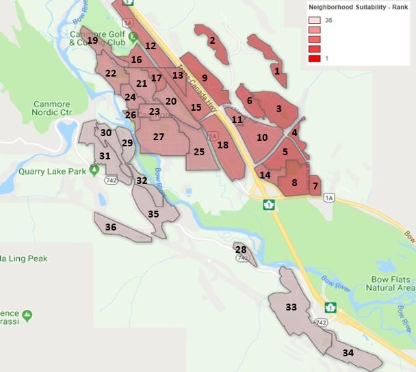
Executive Summary
As climate commitments continue to drive policy decisions around the world, Canmore must explore
alternative energy sources to remain both economically competitive and environmentally conscious.
The following report is a theoretical analysis of rooftop solar applicability in Canmore, on a
neighbourhood by neighbourhood basis. The two goals of the study were to determine the total electric
potential of rooftop solar in Canmore, and to generate Suitability Maps that highlight how the solar
potential changes throughout neighbourhoods in the town. The unique terrain surrounding Canmore
was considered, as well as each neighbourhood’s building types. The data are shown as a relative
ranking in the Suitability Maps, and the numerical values are all presented in Appendix A.

Suitability Maps:
Neighbourhood Suitability - Measures the capacity factor (solar resource potential) of each
neighbourhood’s location within the town.
Building Suitability - Measures the percentage of total rooftop area that could be utilized for solar
arrays.
Net Energy Production - The absolute maximum amount of energy a neighbourhood can generate. Since
this is not levelized based on rooftop areas larger neighbourhoods typically have a larger net energy
production potential.
Overall Suitability - A ranking of how well each neighbourhood is designed for solar taking into account
the neighbourhood and building suitability.
Residential Energy Offset - Measures what percentage of their own electricity residential buildings can
offset per neighbourhood.

Results: If solar was adopted across every possible rooftop in Canmore, the electricity generation would
be 42,181 MWh/yr, which is equivalent to taking 8,600 cars[2] off the road (40,072 tonnesCO2). The
residential sector would, on average, be able to offset 64% of their own electricity usage. Institutional
and commercial buildings do not follow a regular pattern of electricity use, and averages were not be
used to analyze those sectors. The commercial and institutional buildings offer the largest open roof
spaces, therefore offering the largest possible solar systems, which in turn will reduce project costs [7].
Because of these reduced costs on large buildings, an individual analysis of the largest buildings is
recommended.

The analysis presented some interesting, and unexpected results. Most striking was the effect of rooftop
geometry compared to the effect of location within the valley. It was expected to see the sunny eastern
side of the valley significantly out-perform the shady western side, when in fact, the rooftop geometry
ended up having 4.3 times more impact than the location. This reinforces the notion that new
development presents a one-time opportunity to harness solar energy efficiently. These opportunities
can be capitalized on via an update to the architectural guidelines that includes open roof space with
southern exposure. If done correctly, new architectural guidelines can make it easier and cheaper for
residents in Canmore to adopt solar, without sacrificing aesthetics.

                                                                                                          2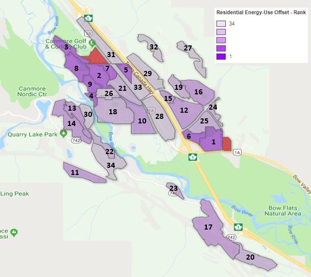
In this analysis, 26 neighbourhoods out of the 36 reviewed were primarily composed of residential
buildings, showing that rooftop solar adoption in Canmore relies heavily on the willingness of
homeowners to install solar arrays. As 75% of building area is zoned for residential-use, the citizens of
Canmore truly have the ability to make a difference in the sustainability of their neighbourhoods.

Ultimately, the conclusion is that the most efficient way to utilize rooftop solar energy in Canmore is to
design rooftops to accommodate solar arrays, prior to breaking ground on a new build. For existing
buildings, the roof design has significantly more impact than location within the valley.

Disclaimer:
The following study is not intended to be used to evaluate an individual residential, commercial, or
municipal project, as the results presented are intended for high-level policy decisions and based on
neighbourhood averages. Each potential site requires an individual assessment by a local professional.

Contact Information:
Collin Ehr - collin.ehr@gmail.com // www.linkedin.com/in/collin-ehr-a857b7120
Taylor Donegan - taylor.donegan@gmail.com // www.linkedin.com/in/taylor-donegan-853541110
Eric Patterson - ericdpatterson8@gmail.com // https://www.linkedin.com/in/eric-patterson-70707b176

                                                                                                             3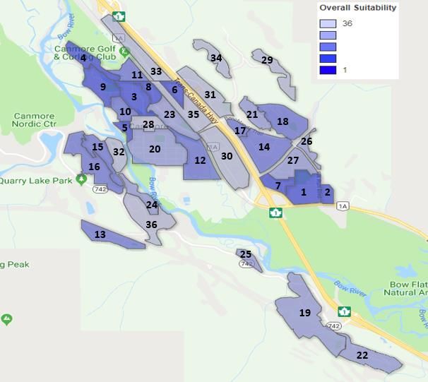
Table of Contents
EXECUTIVE SUMMARY .........................................................................................................................2
    CONTACT INFORMATION: ...................................................................................................................... 3
1.0 - INTRODUCTION ...........................................................................................................................1
2.0 - BACKGROUND .............................................................................................................................1
  2.1 - SOLAR INSTALLATION INCENTIVES ..................................................................................................... 2
3.0 - METHODS ...................................................................................................................................3
  3.1 - BUILDING SUITABILITY METHODOLOGY (APPLICATION FACTOR) ...................................................... 5
  3.2 - NEIGHBOURHOOD SUITABILITY METHODOLOGY (CAPACITY FACTOR).............................................. 7
  3.3 - THEORETICAL MODEL PROCESS AND DATA USED ............................................................................. 8
4.0 – RESULTS .....................................................................................................................................9
     FIGURE 4.1 – NEIGHBOURHOOD SUITABILITY MAP (CAPACITY FACTOR) .............................................11
     FIGURE 4.2 – BUILDING SUITABILITY MAP (APPLICATION FACTOR) .....................................................14
     FIGURE 4.3 – NET SOLAR ENERGY PRODUCTION POTENTIAL (TOTAL OUTPUT) ..................................16
     FIGURE 4.4 – OVERALL SUITABILITY (COMBINED CAPACITY/APPLICATION FACTORS) ......................... 18
     FIGURE 4.5 – RESIDENTIAL ENERGY OFFSET ........................................................................................ 20
     4.6 - POTENTIAL OUTPUT BY SECTOR...................................................................................................22
     4.7 - LEVELIZED ENERGY PRODUCTION ................................................................................................ 23
5.0 – DISCUSSION ON TRENDS FROM THE RESULTS .............................................................................. 24
  5.1 - DIRECTION OF THE PANELS (AZIMUTH) ........................................................................................... 24
  5.2 - EFFECT OF AZIMUTH IN CANMORE ON LEVELIZED COST OF ELECTRICITY.......................................24
  5.3 - LOCATION WITHIN THE BOW VALLEY (TERRAIN SHADING) ............................................................. 25
  5.4 - OFFSETTING RESIDENTIAL ENERGY CONSUMPTION ........................................................................25
  5.5 - A CLOSER LOOK AT SILVERTIP STONECREEK ....................................................................................25
  5.6 - DESIGNING WITH SOLAR IN MIND ...................................................................................................26
  5.7 - THEORETICAL MODEL VS. ACTUAL IMPLEMENTATION....................................................................26
6.0 - RECOMMENDATIONS ................................................................................................................. 27
  6.1 - RECOMMENDATION ON HOW THIS REPORT SHOULD BE USED ......................................................27
  6.2 - RECOMMENDED COURSES OF ACTION............................................................................................ 28
7.0 - CONCLUSION ............................................................................................................................. 30
8.0 - REFERENCES .............................................................................................................................. 31
APPENDIX A: OVERALL RESULTS AND NEIGHBOURHOOD SUMMARIES ......................................................1
      CANMORE’S OVERALL RESULTS: ............................................................................................................ 1
ASPEN ................................................................................................................................................1
AVENS ................................................................................................................................................2
BENCHLANDS TERRACE ........................................................................................................................3
BOW MEADOWS .................................................................................................................................4
BOW VALLEY TRAIL CENTRE ..................................................................................................................5

                                                                                                                                                     4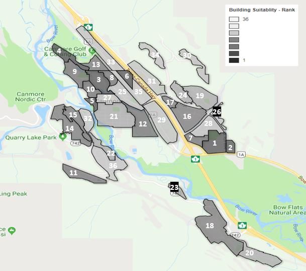
CAIRNS ...............................................................................................................................................6
CANYON RIDGE ...................................................................................................................................7
COUGAR CREEK ...................................................................................................................................8
COUGAR POINT ...................................................................................................................................9
EAGLE TERRACE ................................................................................................................................ 10
ELK RUN ........................................................................................................................................... 11
FAIRHOLM ........................................................................................................................................ 12
GATEWAY ......................................................................................................................................... 13
GROTTO MOUNTAIN VILLAGE ............................................................................................................. 14
HOMESTEADS ................................................................................................................................... 15
INDUSTRIAL PLACE ............................................................................................................................ 16
LARCH .............................................................................................................................................. 17
LION'S PARK...................................................................................................................................... 18
MINESIDE ......................................................................................................................................... 19
NORTH BOW VALLEY TRAIL................................................................................................................. 20
PALLISER .......................................................................................................................................... 21
PEAKS OF GRASSI............................................................................................................................... 22
PROSPECTS ....................................................................................................................................... 23
RIVERSIDE......................................................................................................................................... 24
RUNDLE............................................................................................................................................ 25
RUNDLEVIEW .................................................................................................................................... 26
SILVERTIP LITTLE RAVINE .................................................................................................................... 27
SILVERTIP STONECREEK...................................................................................................................... 28
SOUTH BOW VALLEY TRAIL ................................................................................................................. 29
SOUTH CANMORE ............................................................................................................................. 30
SPRING CREEK................................................................................................................................... 31
SPRING CREEK MOUNTAIN VILLAGE .................................................................................................... 32
STEWART CREEK................................................................................................................................ 33
TEEPEE TOWN................................................................................................................................... 34
THREE SISTERS .................................................................................................................................. 35
TOWN CENTRE .................................................................................................................................. 36
AZIMUTH BREAKDOWN PER NEIGHBOURHOOD (% OF NEIGHBOURHOOD MAXIMUM) ............................ 38
AZIMUTH BREAKDOWN PER NEIGHBOURHOOD (% OF TOWN MAXIMUM).............................................. 39
APPENDIX B: SOLAR SURVEY RESULTS....................................................................................................1
     GOAL 1: NEIGHBOURHOOD UNDERSTANDING ...................................................................................... 1
     GOAL 2: NEIGHBOURHOOD CONCERN ABOUT GHG EMISSIONS ........................................................... 3
     GOAL 3: ACCEPTABLE NEIGHBOURHOOD PAYBACK PERIODS ................................................................ 4

                                                                                                                                                     5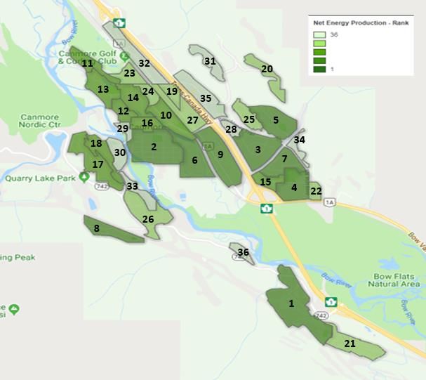
6
1.0 - Introduction
Due to the high level of interest in solar energy from the residents of Canmore (see Appendix B) there is
value in the town exploring the potential of rooftop solar energy and determining the neighbourhoods
best suited for solar arrays. Rooftop solar is an attractive option for renewable electricity in Canmore
due to the lack of available space within the municipality. Knowing the potential of rooftop solar in
Canmore will provide the municipality with a tool that will help to achieve the goals of The
Environmental Sustainability Action Plan (ESAP).

The current GHG emissions associated with Alberta’s electricity grid are approximately
950gCO2eq/kWh[13], the highest in Canada. Given that the average residential building in Alberta
consumes approximately 5.2kWh/ft2[1], Canmore’s total residential electricity consumption is estimated
to be 50,856MWh/year. The associated electricity generation emissions are 48,312tonnes CO2eq/year.
Solar electricity has no generation emissions and as a result could significantly reduce the municipality’s
total emissions. Larger building types (institutional and commercial) do not follow regular energy use
profiles, and so average values do not apply to Canmore’s industrial and commercial district. Accurate
energy data on Canmore’s commercial and institutional buildings was not available, though there are
many options for tracking this type of data, such as third-party energy-tracking services.

One of the largest deterrents in solar energy adoption is the installation costs and associated high
payback periods. To minimize the payback period and maximize the return on investment it is important
to install solar arrays in the areas with the highest solar potential. In pursuit of this, this study provides a
relative ranking of neighbourhoods in Canmore based on their solar suitability. This will provide the
municipality with information on how they can target their investment, subsidies, and education
programs to maximize the emissions offset by solar arrays. An overall rooftop production potential has
also been provided to allow the town to assess the potential impact of investing in solar generation.
Interestingly the percentage difference between the neighbourhood with the highest average capacity
factor, Silvertip Stonecreek, and the lowest average capacity factor, Peaks of Grassi, is only 11.4%. This
demonstrates that the impact of mountain shading may not be as significant as one would think. When
comparing the maximum capacity factors at an ideal azimuth (typically 180 degrees) in each
neighbourhood the percentage difference increases to 17.3%.

2.0 - Background
Alberta’s electrical grid relies on carbon intensive generation sources such as coal and natural gas,
resulting in a grid with greenhouse gas emission intensity 5 times the national average [3]. To reduce the
greenhouse gas intensity, cleaner generation sources must be added to the generation mix. Southern
Alberta has some of the highest solar irradiance (watts/m2 from the sun) levels in North America,
making it an attractive location for solar generation. Solar generation has lifecycle emissions over 30
times less than coal, and 10 times less than natural gas[4]. The combination of high solar potential and
low emissions makes solar generation an attractive option for low-carbon electricity generation.

                                                                                                               1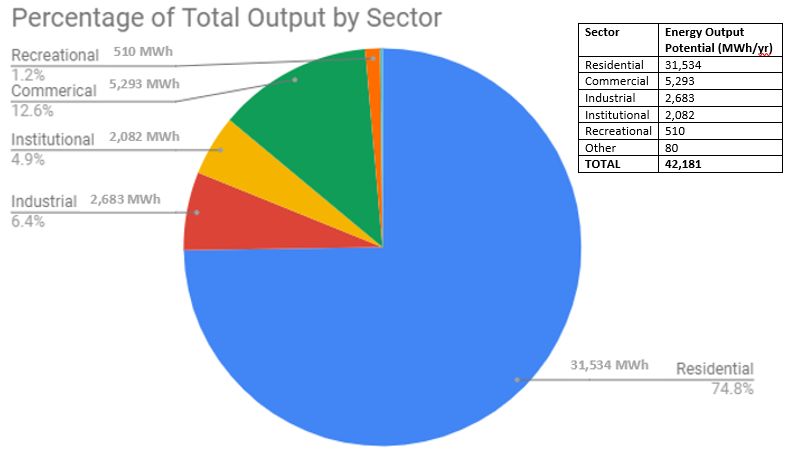
Solar electricity generation can be classified as either utility scale (large) or microgeneration (small).
Municipalities are generally concerned with microgeneration, particularly rooftop generation, to
increase the utility of already occupied space. This generation is usually tied into the electrical grid so
that in times of excess supply, the electricity is exported to the grid and made available to all consumers.
The producer is then given a credit on their electricity bill for electricity added to the grid. Conversely, in
times of low supply, the grid can supplement the production of the solar array, removing the need for
battery storage. Adding large, variable amounts of electricity to the grid could create complications for
the grid operators. However, since Alberta has a large interconnected grid, the impact of a single
municipality on the overall generation and consumption within the province is negligible. As a result, the
variable nature of grid connected solar systems is mitigated and the overall impact to the Alberta grid is
minimal. The downside to an individual producing electricity and exporting to the grid instead of
consuming it locally is that the transmission and distribution charges associated with electricity use are
not avoided. It is within provincial law that Albertans can install only enough microgeneration to cover
their own consumption. Annual production cannot exceed annual consumption[5].

2.1 - Solar Installation Incentives
With available subsidies (seen in Table 2.1) and rapidly decreasing costs, solar energy is becoming
increasingly affordable. Although Alberta’s electricity prices are currently among the lowest in the
world, uncertainty surrounding the future of the electricity market following the retirement of the coal
facilities could increase the economic viability of solar energy and provide a buffer against rising
electricity rates. Additionally, the town of Canmore offered eight solar subsidies with a value of $1250
each in 2018 to further incentivize rooftop solar in the municipality. As can be seen in Appendix B,
knowledge of both the provincial and municipal incentives in Canmore is low. A potential use of this
study is to target education/information campaigns toward citizens living in areas with high solar
suitability.

Table 2.1: Existing Solar Subsidies as of September 2018:
                                                  Residential                            Commercial

Provincial Maximum Incentives        The lesser of $10 000, or 30% of eligible   The lesser of $500 000,
                                                   system costs                     or 25% of eligible
                                                                                      system costs
      Municipal Incentives            Eight subsidies of $1250, given based on lottery after application

                                                                                                             2
3.0 - Methods
Our theoretical model of Canmore’s rooftop solar energy includes two main sets of factors: Application
(building suitability) and Capacity (neighbourhood suitability). The Capacity Factor methodology has
been verified with existing solar arrays in Canmore. It was found to be quite accurate with a cumulative
error of 1.04%, as shown in Table 3.1. The Application Factor is mainly a function of roof design and
varies greatly based on the style of construction. Neighbourhoods with high Application Factors
represent construction styles that favour solar arrays.

Important Assumptions:
    1) Roofs were assumed to have an equal likelihood of facing any direction and trend areas were
       used for any significant group of roofs that clearly did not follow this assumption.
    2) Any roof area that could not contain at least 6 panels was assumed to not have any panels due
       to economic constraints[6].
    3) Assumed standard 5.25 x 3.3ft, 280W panel[6]: REC 280W, this is the panel most commonly used
       by Skyfire Energy.
    4) Average roof tilt is assumed to be 27 degrees based on the recommendation of the Bow Valley
       Builders and Development Association. This assumption was validated by the solar array
       installation data provided by KCP Energy. Setting these variables allows the measurement of
       variation based on location (see section 3.2).

Relevant Definitions:
    •   Insolation: The amount of solar radiation that reaches the earth's surface. The available
        insolation determines how much output a solar panel will produce throughout the day.
    •   Azimuth: The horizontal direction, in degrees, the panel faces. 0/360 degrees represents a panel
        facing due north and 180 degrees represents a panel facing due south.
    •   Tilt: The vertical orientation of the panel. 0 degrees would represent a flat panel and 90 degrees
        would represent a vertical panel.
    •   Application Factor: Application Factors are applied to reduce the amount of total rooftop area to
        an area suitable for PV panel installation. This is a measure of usable rooftop area (also referred
        to as ‘Building Suitability’ in this report).
    •   Capacity Factor: The Capacity Factor converts the installed power of a solar array into electricity
        generation. It represents the actual electricity production as a percentage of the theoretical
        maximum production over a given time period. For the purposes of this report the Capacity
        Factor is an annualized value providing the average electricity generation potential throughout
        the course of the year. The Capacity Factor takes into account the amount of electricity
        generation for the amount of solar insolation at a given location, tilt, and azimuth. Capacity
        Factor is also referred to as ‘Neighbourhood Suitability’ in this report.
    •   Trends: A trend in a neighbourhood is defined as any set of buildings that do not follow the
        assumption that all roof planes are equally likely to face all directions. Identifying trends in
        neighbourhoods allows this report’s analysis to account for regular, repeating construction types

                                                                                                           3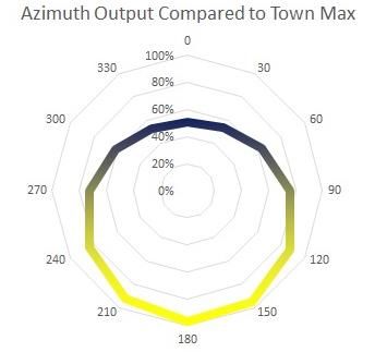
(condos, low income housing, storage units, etc.) without abandoning our assumptions for
        average neighbourhoods.

Table 3.1: Theoretical Production vs. Actual Production
 Site Name      Latitude       Longitude     Array Size   Average      Prediction using   % Difference
                                             (kW)         Actual       Theoretical
                                                          Production   Model (kWh)
                                                          (kWh)

 9 Street       51.090226      -115.36414    6.24         4456.9       4556.4             -0.55%

 9 Street       51.0901393     -115.36478    5.46         5182.5       5044.5             0.67%

 11 Street      51.0914229     -115.36543    8.58         9756.6       9019.3             1.96%

 Larch Place    51.1034273     -115.37806    3.66         3269.8       3745.3             -3.39%

 Cougar Point   51.088754      -115.33867    4.77         4764.4       4874.5             -0.57%
 Road

 Coyote Way     51.0863092     -115.32892    4.42         4808.5       4577.8             1.23%

 Lady           51.084064      -115.32795    3.66         4190.6       3556.25            4.09%
 Macdonald
 Crescent

 Larch Avenue   51.1001695     -115.37237    4.24         3507.2       4202.7             -4.51%

 Miskow         51.057621      -115.32824    6.71         6866.0       5718.3             4.56%
 Close

 2nd Street     51.0837466     -115.35954    4.88         5285.9       5023               1.28%

 Moraine        51.0808404     -115.32722    3.71         4509.1       3983.4             3.10%
 Road

 Overall:                                                 56597.5      54301.45           1.04%

                                                                                                         4
3.1 - Building Suitability Methodology (Application Factor)
To calculate the amount of area in Canmore that is available for rooftop solar, the percentage of usable
roof area was determined in each neighbourhood. This was done by applying the Application Factors
listed below to an appropriate number of homes, determined based on the size of the neighbourhood,
and averaging the result. The overall confidence interval is 6.5% for the Application Factor results. For
neighbourhoods with trend areas, additional sample buildings that mirrored the trend were averaged
separately. The trend areas were then calculated as a percentage of the total neighbourhood area and a
weighted average was used to determine the overall neighbourhood Application Factor. The overall
Application Factor ranking by neighbourhood can be seen in Figure 4.2, in the Results section. The
Application Factor values can be found in Appendix A, separated by neighbourhood. The following
factors were applied to their neighbourhood’s total area, resulting in a realistic area available for
rooftop solar.
Application Factors Considered:
Obstacles - This factor represents the amount of usable roof area accounting for areas that are already
in use for chimneys, HVAC systems, and geometry. CONNECTExplore software (provided by the town of
Canmore) was used for sample building roof measurements, and steps are outlined below. Obstacle
factor methodology was verified when possible by visually inspecting existing arrays and comparing the
actual number of panels to the expected number of panels for the building. There were no significant
discrepancies.
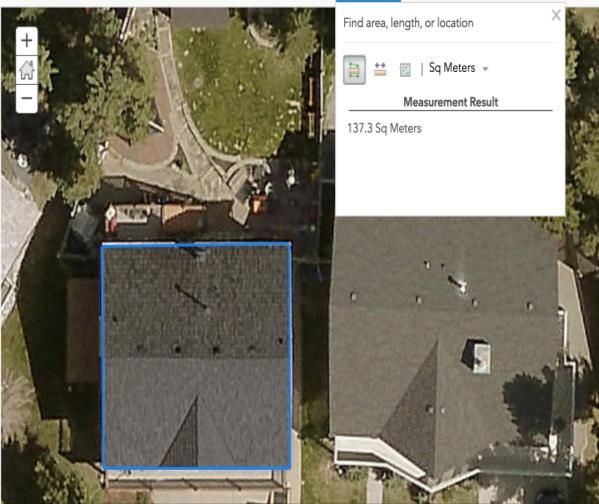
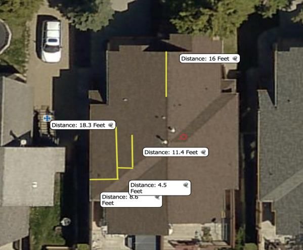
Step 1 - Determine the total roof area of a sample building by using the CONNECTExplore ‘area’ tool.
Step 2 - Determine the length and width of any roof plane on the sample building roof using the
CONNECTExplore ‘distance’ tool, a sample is shown below in Figure 3.1
Figure 3.1: Steps 1 and 2 in Obstacle Factor determination
5Step 3 - Calculate the maximum number of standard 5.25 x 3.3ft panels that could be placed in each
open space, either by placing them on a vertical or horizontal orientation. If the maximum number of
panels was less than 6, assume no panels would be placed in this area as systems less than 1.5kW
(6x280W panels) are not economic.
Step 4 - Add up the number of panels for all the areas on the sample building and convert to area by
multiplying by the area of a standard 5.25 x 3.3ft, 280W panel.
Step 5 - Divide the maximum panel area by the total roof area to calculate the overall obstacle factor for
the sample building.
Step 6 - Repeat steps 1-5 for an appropriate number of sample buildings and calculate the average
value. Do the same for each trend.
Shading - The shading value was kept consistent at 63%[6], meaning that 37% of roof area is not fit for
solar due to excess shading from objects such as trees or other buildings. This value is from a 2016 NREL
report[6] that found the solar potential in the US by using LIDAR data for buildings in 128 US cities
(approximately 23% of all US buildings). Any area that had an isolation level less than 80% of the
maximum insolation in that area was considered unfit for solar due to shading. The Canmore specific
shading value may differ slightly, but this was beyond the scope of the project.
Structural Applicability - This factor takes into account the ability of the building to support the
additional load of the solar panels. A value of 95% (5% unsuitable) was chosen for residential buildings
and 85% (15% unsuitable) was chosen for larger commercial and institutional buildings. These numbers
are based on consultation with Skyfire Energy and KCP, two of the leading solar installers in the province
of Alberta. The material used in the construction of each building type plays a role in the difference
between factors.
Array Type – This factor accounts for the unusable roof area from panel spacing and self-shading. There
are two types of arrays that were considered, open rack and fixed mount. Open rack panels are used on
flat rooftops, to increase the tilt. Fixed mount panels are installed directly onto the roof plane. Open
rack panels cast a larger shadow than fixed mounted panels, resulting in less usable roof space. The
values of 98% (2% unusable) for fixed mounted and 70% (30% unusable) for open rack were taken from
the same NREL report referenced in the ‘Shading’ section.
63.2 - Neighbourhood Suitability Methodology (Capacity Factor)
Once the total usable rooftop area for solar installations was found through section 3.1, the next step
was to calculate the output of the solar arrays in Canmore based on their locations in the town. A
combination of data from existing solar arrays in Canmore, the software SolarGIS, and available
literature was used. The overall Capacity Factor ranking by neighbourhood can be seen in Figure 4.1, in
the Results section. The Capacity Factor values can be found in Appendix A, separated by
neighbourhood. Steps in the analysis are outlined below.
Step 1 - SolarGIS data points were taken at an average interval of 250 meters around the perimeter of
each neighbourhood. The 250m interval was chosen to match the resolution of the SolarGIS software.
The average number of data points considered per neighbourhood was 13.
Step 2 - SolarGIS software was used to view the annual solar insolation for each of the 473 data points
within the town of Canmore.
- To ensure consistency across all measurements, an azimuth angle of 180 degrees and a
tilt angle of 27 degrees were assumed. The 27 degree tilt was recommended by the Bow
Valley Builders and Development Association as an average tilt for houses in Canmore.
This was validated as the average tilt of the reference arrays provided by KCP energy
was 27 degrees.
- For each point, the total available solar insolation was considered as well as the
percentage reduced by terrain shading (mountains) and percentage reduced by angular
reflectivity.
Step 3 - To account for the assumption that all roof planes are equally likely to face all directions, data
points at 12 different azimuth angles (0, 30, 60, 90, 120, 150, 180, 210, 240, 270, 300, 330) were taken in
the center of each neighbourhood and the output was calculated using SolarGIS data. This shows the
variation in output as the panels face different directions. For the purposes of our results the average of
the output at each of the 12 different azimuth angles was used as the average output for each
neighbourhood.
Step 4 - Data was exported from SolarGIS and system losses of 12%[7] were applied, taking into account:
soiling, shading, mismatch, wiring, connections, degradation, slight inaccuracies in the accuracy of
manufacturer panel rating and system availability.
- Inverter losses of 4%[7] were applied for the conversion of DC to AC electricity.
- Snow losses were calculated using the NAIT reference array data for Edmonton[8] and
the difference in precipitation between Canmore and Edmonton. This was completed by
multiplying the annual losses due to snow of 4.04% at a 27 degree tilt in Edmonton by
the difference between Edmonton and Canmore precipitation between November and
March (assumed as months with snow). The resulting annual snow losses in Canmore
were 7.57%.
73.3 - Theoretical Model Process and Data Used
To compare the results of Building and Neighbourhood suitability the data was combined and analyzed
on a neighbourhood by neighbourhood basis. The following procedure outlines how the overall model
of the town was designed and includes information on the data inputs for this process.
Modelling Process:
1) Total Roof Area: To calculate the total roof area the total building area was used as well as the
assumption that the average building roof was tilted at an angle of 27 degrees. The roof area was
broken down by neighbourhood and by building classification (residential, commercial, industrial,
institutional, recreational, and other).
2) Usable Roof Area: To calculate the total available space on each rooftop that could be used for solar
energy, the total roof area was multiplied by the Building Suitability (Application Factor) to give a
usable roof area for solar energy in each neighbourhood.
3) Installed Power: The usable roof area was divided by the area requirements for a single solar panel
and then multiplied by the rated capacity of the assumed solar panel to give an installed power
value in Watts.
4) Electricity Output: The installed power was converted to annual electricity production using the
Capacity Factor and the assumption that each panel is equally likely to be facing any direction
(north, south, east, west). The installed power was multiplied by the capacity factor and the number
of hours in the year to provide the annual electricity production in kWh. The individual Capacity and
Application Factors for each neighbourhood were used and the results were summed to calculate
the solar potential for the entire town.
5) Overall Solar Suitability: The output per meter squared of building area combines the Capacity and
Application Factors to show which neighbourhoods have the highest output potential per meter
squared of building area. This should not be confused with efficiency of a panel installed in a given
location which is represented by Capacity factor.
6) Average Array Size: The average residential array size was calculated using the total residential
building area in each neighbourhood divided by the number of residential structures in the
neighbourhood. Using the roof angle assumption and applicable Application Factors the average
array size was calculated.
7) Percentage of Residential Electricity Offset: The percentage of residential electricity usage that could
be offset by maximizing the solar installations on residential buildings in each neighbourhood. This
was calculated by multiplying the average residential array size in each neighbourhood by the
number of residential structures and then using the Capacity Factor to calculate the electricity
production. The percentage offset was based on the Energy Efficiency Alberta guidepost that each
single detached home uses, on average, 5.2kWh/ft2 of building area[1].
8Data sources include:
CONNECTExplore software: Used for the calculation of the Application Factor (building suitability) and
analysis of individual buildings suitability for solar.
SolarGIS: Used to provide solar insolation data for locations across Canmore and show the variation of
available solar energy across the town and how it varies with azimuth angle.
Edmonton Snow Loading study & Canmore Weather Data: Used to estimate the impact of losses due to
snow in the town of Canmore. This data is open-sourced.
PVWatts: NREL database used for system and inverter losses.
Building footprint area data (Canmore): Used to estimate total rooftop area available in the town of
Canmore.
Building usage/class/neighbourhood data (Canmore): Used to categorize the results into building usage,
neighbourhood, building class data.
KCP Energy output from existing arrays: Used to validate our model by comparing the output of our
model to existing solar arrays in Canmore.
4.0 – Results
The results of this study are presented in five Suitability Maps and two other figures. Together, these
visuals show the variation in solar-applicability across the town. It is important to note that all the
Suitability Maps are ranked relative to the town’s maximum. To see just how much each neighbourhood
varies, a breakdown is shown in Appendix A.
To generate the Suitability Maps, Google’s Fusion Tables were used. These tables allow the reader of
this study to interact with the Suitability Maps (if an electronic copy is available), simply follow the
appropriate link, select the maps tab, and select a neighbourhood to see the exact ranking. The shapes
and lengths represent neighbourhood boundaries as described by KML data provided via the town of
Canmore.
Figure 4.1 – Neighbourhood Suitability Map
Figure 4.2 – Building Suitability Map
Figure 4.3 – Net Energy Production (Production Potential/ Overall Output)
Figure 4.4 – Overall Suitability
Figure 4.5 – Residential Energy Offset
9Figure 4.0: Neighbourhood Reference Map
Town of Canmore - Neighbourhoods
East
North Bow
Valley
Trail Silvertip
Larch Ravine
Industrial Silvertip
Place Stonecreek
Lion's Teepee
As p
Park Spring Town Palliser
en
Creek
Fairholm G Bow Valley
at
Benchlands
ew Trail
Town Terrace ayEagle
Centre
Town Boundary
River- CentreCougar Terrace
side Point
Mineside South South Canyon
Bow Valley Cougar
Rundle
Canmore Creek Ridge
Trail
Rundle- Spring Creek
view Avens
Mountain
Village Grotto
Mountain Elk Run
ro
P
sp Village
Bow
ec
s Meadows
t
Homesteads
Peaks of
Grassi
Cairns
Three
Sisters
Proposed Land Use Redesignation Stewart
Creek
500 Neighbourhoods
250 0 500 Meters
Date: 12/3/2018 Name: FCL2017_01_Neighbourhoods_DB Map produced by Town of Canmore GIS Services
10Figure 4.1 – Neighbourhood Suitability Map (Capacity Factor)
The Neighbourhood Suitability map shows the capacity factor of each neighbourhood. The capacity
factor is representative of the percentage of time a solar panel on a roof in the neighbourhood would be
producing at its maximum rated output. The higher the capacity factor, the more solar irradiation
(sunlight) is available in the neighbourhood over the course of the year, which increases the efficiency of
rooftop solar installations. This map can show where the highest natural potential for solar is within the
town, however this does not necessarily correlate to the areas with the highest available usable rooftop
area for solar. The neighbourhood of Silvertip Stonecreek is the most suitable location for solar, with a
Capacity factor of 13.18% at a 180 degree azimuth. Peaks of Grassi is the least suitable with a Capacity
factor of 11.08% at a 180 degree azimuth. A complete neighbourhood breakdown can be found in
Appendix A. It can be seen from Figure 4.1 that neighbourhoods in the northeast tend to have better
solar production potential, gradually becoming less suitable the farther southwest they are. This is due
to the unique shading provided to Canmore from the surrounding mountains. The northeast section of
the town receives more hours of sunlight than the southwest portion. This does not mean that the
southwestern neighbourhoods are necessarily bad for solar. Southern Alberta has a higher solar
insolation (W/m2) than the capital cities in Germany and China[9], the countries with the most installed
solar capacity worldwide. Even the worst neighbourhoods in Canmore have a relatively high potential.
1112
Community Value/Rank Maximum Community Capacity Factor (180 Degrees) Average Community Capacity Factor (Cumulative)
Aspen Value 12.65% 9.67%
Aspen Rank 17 18
Avens Value 12.88% 9.77%
Avens Rank 5 6
Benchlands Terrace Value 12.87% 9.76%
Benchlands Terrace Rank 6 7
Bow Meadows Value 12.87% 9.75%
Bow Meadows Rank 7 8
Bow Valley Trail Centre Value 12.71% 9.73%
Bow Valley Trail Centre Rank 15 13
Cairns Value 12.15% 9.48%
Cairns Rank 28 28
Canyon Ridge Value 12.96% 9.77%
Canyon Ridge Rank 4 5
Cougar Creek Value 12.83% 9.73%
Cougar Creek Rank 9 12
Cougar Point Value 12.80% 9.74%
Cougar Point Rank 12 10
Eagle Terrace Value 13.02% 9.80%
Eagle Terrace Rank 3 3
Elk Run Value 12.84% 9.78%
Elk Run Rank 8 4
Fairholm Value 12.48% 9.62%
Fairholm Rank 25 23
Gateway Value 12.61% 9.67%
Gateway Rank 20 17
Grotto Mountain Village Value 12.75% 9.72%
Grotto Mountain Village Rank 13 15
Homesteads Value 11.78% 9.24%
Homesteads Rank 34 35
Industrial Place Value 12.69% 9.66%
Industrial Place Rank 16 21
Larch Value 12.63% 9.66%
Larch Rank 19 20
Lion's Park Value 12.54% 9.61%
Lion's Park Rank 22 24
Mineside Value 12.04% 9.39%
Mineside Rank 30 30
North Bow Valley Trail Value 12.81% 9.72%
North Bow Valley Trail Rank 11 14
Paliser Value 12.82% 9.75%
Paliser Rank 10 9
Peaks of Grassi Value 11.08% 8.85%
Peaks of Grassi Rank 36 36
Prospects Value 11.93% 9.34%
Prospects Rank 32 32
Riverside Value 12.36% 9.56%
Riverside Rank 27 26
Rundle Value 12.13% 9.44%
Rundle Rank 29 29
Rundleview Value 11.96% 9.34%
Rundleview Rank 31 33
Silver Tip Ravine Value 13.02% 9.84%
Silver Tip Ravine Rank 2 2
Silvertip Stonecreek Value 13.18% 9.91%
Silvertip Stonecreek Rank 1 1
South Bow Valley Trail Value 12.63% 9.69%
South Bow Valley Trail Rank 18 16
South Canmore Value 12.38% 9.55%
South Canmore Rank 26 27
Spring Creek Value 12.59% 9.67%
Spring Creek Rank 21 19
Spring Creek Mountain Village Value 12.49% 9.60%
Spring Creek Mountain Village Rank 24 25
Stewart Creek Value 11.69% 9.34%
Stewart Creek Rank 35 34
Teepee Town Value 12.75% 9.73%
Teepee Town Rank 14 11
Three Sisters Value 11.78% 9.36%
Three Sisters Rank 33 31
Town Centre Value 12.49% 9.63%
Town Centre Rank 23 22
Canmore Overall Value 12.51% 9.61%
13Figure 4.2 – Building Suitability Map (Application Factor)
The Building Suitability map shows the application factor of each of the neighbourhoods. The application
factor represents the percentage of the overall rooftop area that is suitable for solar installations.
Neighbourhoods with higher application factors have larger unobstructed rooftop area that could be
used for solar installations increasing the output potential of the neighbourhood. The neighbourhood of
Elk Run has the highest ratio of roof area available for solar compared to total roof area, with an
Application Factor of 45.74%. Homesteads has the lowest Application Factor with only 8.97% of roof
area being usable for solar production. A complete neighbourhood breakdown can be found in Appendix
A. Neighbourhoods with a high percentage of institutional/industrial buildings tend to have a better
ranking due to a higher ‘Obstacles’ factor (less obstacles in the way). The large, open roof spaces allow
for larger groups of panels while many residential homes have open areas too small to fit at least 6
panels on. There are however, many unique factors involved in calculating the Application Factor which
results in the lack of trend, as seen in Figure 4.2.
14Community Value/Rank Application Factor
Aspen Value 30.87%
Aspen Rank 8
Avens Value 18.01%
Avens Rank 28
Benchlands Terrace Value 19.33%
Benchlands Terrace Rank 24
Bow Meadows Value 41.04%
Bow Meadows Rank 2
Bow Valley Trail Centre Value 10.71%
Bow Valley Trail Centre Rank 35
Cairns Value 19.36%
Cairns Rank 23
Canyon Ridge Value 18.36%
Canyon Ridge Rank 26
Cougar Creek Value 24.68%
Cougar Creek Rank 16
Cougar Point Value 21.14%
Cougar Point Rank 17
Eagle Terrace Value 20.39%
Eagle Terrace Rank 19
Elk Run Value 45.74%
Elk Run Rank 1
Fairholm Value 28.31%
Fairholm Rank 10
Gateway Value 19.20%
Gateway Rank 25
Grotto Mountain Village Value 31.88%
Grotto Mountain Village Rank 7
Homesteads Value 8.97%
Homesteads Rank 36
Industrial Place Value 26.25%
Industrial Place Rank 13
Larch Value 34.24%
Larch Rank 4
Lion's Park Value 29.00%
Lion's Park Rank 9
Mineside Value 24.92%
Mineside Rank 15
North Bow Valley Trail Value 13.14%
North Bow Valley Trail Rank 33
Paliser Value 14.44%
Paliser Rank 31
Peaks of Grassi Value 27.79%
Peaks of Grassi Rank 11
Prospects Value 19.72%
Prospects Rank 22
Riverside Value 33.43%
Riverside Rank 5
Rundle Value 13.84%
Rundle Rank 32
Rundleview Value 25.01%
Rundleview Rank 14
Silver Tip Ravine Value 12.96%
Silver Tip Ravine Rank 34
Silvertip Stonecreek Value 15.88%
Silvertip Stonecreek Rank 30
South Bow Valley Trail Value 15.94%
South Bow Valley Trail Rank 29
South Canmore Value 19.90%
South Canmore Rank 21
Spring Creek Value 34.51%
Spring Creek Rank 3
Spring Creek Mountain Village Value 26.36%
Spring Creek Mountain Village Rank 12
Stewart Creek Value 20.01%
Stewart Creek Rank 20
Teepee Town Value 32.03%
Teepee Town Rank 6
Three Sisters Value 20.94%
Three Sisters Rank 18
Town Centre Value 18.05%
Town Centre Rank 27
Canmore Overall Value 23.23%
15Figure 4.3 – Net Solar Energy Production Potential (Total Output)
With 100% adoption of solar on all rooftops that meet criteria (outlined in section 3.1), the total solar
energy production potential for the town of Canmore is 42,181 MWh/yr, offsetting 40,072
tonnesCO2eq/yr. It should be noted that the net solar energy production is significantly impacted by the
size of each neighbourhood. This should not be confused with a metric showing the quality of each
neighbourhood for solar energy production. It is meant to show a snapshot of the total electricity each
neighbourhood could produce if solar arrays were maximized on all existing structures. This is a
combination of the Building and Neighbourhood Suitability maps above. Assuming that residential
homes in Canmore consume the same amount of electricity per square foot as an average Alberta
home, each neighbourhood could offset an average of 64% of its own residential electricity use with
rooftop solar generation. The neighbourhood potential output rank can be seen in Figure 4.3. The
neighbourhoods with the highest and lowest production potential respectively are Three Sisters (3,339
MWh/yr) and Cairns (171 MWh/yr). A complete neighbourhood breakdown can be found in Appendix A.
16Community Value/Rank Total Output (MWh/year)
Aspen Value 872.07
Aspen Rank 24
Avens Value 1650.80
Avens Rank 7
Benchlands Terrace Value 747.51
Benchlands Terrace Rank 25
Bow Meadows Value 889.54
Bow Meadows Rank 22
Bow Valley Trail Centre Value 611.24
Bow Valley Trail Centre Rank 27
Cairns Value 171.40
Cairns Rank 36
Canyon Ridge Value 446.05
Canyon Ridge Rank 34
Cougar Creek Value 2746.53
Cougar Creek Rank 3
Cougar Point Value 562.13
Cougar Point Rank 28
Eagle Terrace Value 1990.72
Eagle Terrace Rank 5
Elk Run Value 2062.87
Elk Run Rank 4
Fairholm Value 1258.57
Fairholm Rank 12
Gateway Value 1428.47
Gateway Rank 10
Grotto Mountain Village Value 1085.53
Grotto Mountain Village Rank 15
Homesteads Value 707.02
Homesteads Rank 26
Industrial Place Value 873.10
Industrial Place Rank 23
Larch Value 1415.46
Larch Rank 11
Lion's Park Value 1245.05
Lion's Park Rank 13
Mineside Value 1028.08
Mineside Rank 18
North Bow Valley Trail Value 470.08
North Bow Valley Trail Rank 32
Paliser Value 242.96
Paliser Rank 35
Peaks of Grassi Value 1646.52
Peaks of Grassi Rank 8
Prospects Value 449.09
Prospects Rank 33
Riverside Value 560.40
Riverside Rank 29
Rundle Value 484.47
Rundle Rank 30
Rundleview Value 1038.77
Rundleview Rank 17
Silver Tip Ravine Value 478.63
Silver Tip Ravine Rank 31
Silvertip Stonecreek Value 937.31
Silvertip Stonecreek Rank 20
South Bow Valley Trail Value 1567.27
South Bow Valley Trail Rank 9
South Canmore Value 3235.02
South Canmore Rank 2
Spring Creek Value 1219.75
Spring Creek Rank 14
Spring Creek Mountain Village Value 1735.46
Spring Creek Mountain Village Rank 6
Stewart Creek Value 922.81
Stewart Creek Rank 21
Teepee Town Value 993.94
Teepee Town Rank 19
Three Sisters Value 3338.53
Three Sisters Rank 1
Town Centre Value 1067.93
Town Centre Rank 16
Canmore Overall Value 42181.07
17Figure 4.4 – Overall Suitability (Combined Capacity/Application Factors)
The overall suitability combines the capacity and application factors. It calculates the total electricity
output (kWh) per m2 of rooftop area. It takes into account both the number of panels that could be
placed on a rooftop given the application factor guidelines and multiples that by the average capacity
factor of the installed panels. It does not take into account the size of a neighbourhood, just the average
overall quality of a rooftop for solar energy. Figure 4.4 shows the neighbourhood ranking for solar
generation per unit of roof area. This differs from overall potential in that it allows neighbourhoods to
be compared in a levelized way, factoring both Building and Neighbourhood suitability. Elk Run has
73.75 kWh/m2/yr, the highest neighbourhood levelized potential output. Homesteads has the lowest
levelized potential output with 13.66 kWh/m2/yr. A complete neighbourhood breakdown can be found
in Appendix A. Canmore’s overall solar potential per unit of roof area is 36.80 kWh/m2/yr. The Overall
Suitability Map closely mirrors the Building Suitability Map, suggesting that building type has a greater
impact on existing neighbourhoods than location within the valley.
18Community Value/Rank Overall Suitability (kWh/m2/year)
Aspen Value 49.21
Aspen Rank 8
Avens Value 29.00
Avens Rank 27
Benchlands Terrace Value 31.08
Benchlands Terrace Rank 21
Bow Meadows Value 65.94
Bow Meadows Rank 2
Bow Valley Trail Centre Value 17.17
Bow Valley Trail Centre Rank 35
Cairns Value 30.25
Cairns Rank 25
Canyon Ridge Value 29.57
Canyon Ridge Rank 26
Cougar Creek Value 39.57
Cougar Creek Rank 14
Cougar Point Value 33.95
Cougar Point Rank 17
Eagle Terrace Value 32.95
Eagle Terrace Rank 18
Elk Run Value 73.75
Elk Run Rank 1
Fairholm Value 44.89
Fairholm Rank 10
Gateway Value 30.61
Gateway Rank 23
Grotto Mountain Village Value 51.09
Grotto Mountain Village Rank 7
Homesteads Value 13.66
Homesteads Rank 36
Industrial Place Value 41.79
Industrial Place Rank 11
Larch Value 54.54
Larch Rank 4
Lion's Park Value 45.92
Lion's Park Rank 9
Mineside Value 38.56
Mineside Rank 15
North Bow Valley Trail Value 21.06
North Bow Valley Trail Rank 33
Paliser Value 23.20
Paliser Rank 31
Peaks of Grassi Value 40.52
Peaks of Grassi Rank 13
Prospects Value 30.38
Prospects Rank 24
Riverside Value 52.68
Riverside Rank 5
Rundle Value 21.53
Rundle Rank 32
Rundleview Value 38.49
Rundleview Rank 16
Silver Tip Ravine Value 21.02
Silver Tip Ravine Rank 34
Silvertip Stonecreek Value 25.95
Silvertip Stonecreek Rank 29
South Bow Valley Trail Value 25.46
South Bow Valley Trail Rank 30
South Canmore Value 31.31
South Canmore Rank 20
Spring Creek Value 55.01
Spring Creek Rank 3
Spring Creek Mountain Village Value 41.71
Spring Creek Mountain Village Rank 12
Stewart Creek Value 30.79
Stewart Creek Rank 22
Teepee Town Value 51.37
Teepee Town Rank 6
Three Sisters Value 32.29
Three Sisters Rank 19
Town Centre Value 28.65
Town Centre Rank 28
Canmore Overall Value 36.80
19Figure 4.5 – Residential Energy Offset
Figure 4.5 represents a ranking of each neighbourhoods ability to offset their own residential electricity
usage (areas in red have no residential). This potential would only be realized if solar panels were
installed on all available residential rooftop area that met the criteria of the application factors. The
neighbourhood of Elk Run has the greatest residential electricity offset and Homesteads has the least
offset. A complete neighbourhood breakdown can be found in Appendix A.
20Community Value/Rank Residential % Energy Offset
Aspen Value 87.93%
Aspen Rank 7
Avens Value 51.80%
Avens Rank 25
Benchlands Terrace Value 55.53%
Benchlands Terrace Rank 19
Bow Meadows Value
Bow Meadows Rank
Bow Valley Trail Centre Value 30.68%
Bow Valley Trail Centre Rank 33
Cairns Value 54.04%
Cairns Rank 23
Canyon Ridge Value 52.83%
Canyon Ridge Rank 24
Cougar Creek Value 70.70%
Cougar Creek Rank 12
Cougar Point Value 60.65%
Cougar Point Rank 15
Eagle Terrace Value 58.88%
Eagle Terrace Rank 16
Elk Run Value 131.76%
Elk Run Rank 1
Fairholm Value 80.20%
Fairholm Rank 9
Gateway Value 54.69%
Gateway Rank 21
Grotto Mountain Village Value 91.29%
Grotto Mountain Village Rank 6
Homesteads Value 24.41%
Homesteads Rank 34
Industrial Place Value
Industrial Place Rank
Larch Value 97.44%
Larch Rank 3
Lion's Park Value 82.04%
Lion's Park Rank 8
Mineside Value 68.90%
Mineside Rank 13
North Bow Valley Trail Value 37.63%
North Bow Valley Trail Rank 31
Paliser Value 41.44%
Paliser Rank 29
Peaks of Grassi Value 72.40%
Peaks of Grassi Rank 11
Prospects Value 54.27%
Prospects Rank 22
Riverside Value 94.12%
Riverside Rank 4
Rundle Value 38.46%
Rundle Rank 30
Rundleview Value 68.78%
Rundleview Rank 14
Silver Tip Ravine Value 37.56%
Silver Tip Ravine Rank 32
Silvertip Stonecreek Value 46.37%
Silvertip Stonecreek Rank 27
South Bow Valley Trail Value 45.49%
South Bow Valley Trail Rank 28
South Canmore Value 55.94%
South Canmore Rank 18
Spring Creek Value 98.29%
Spring Creek Rank 2
Spring Creek Mountain Village Value 74.52%
Spring Creek Mountain Village Rank 10
Stewart Creek Value 55.02%
Stewart Creek Rank 20
Teepee Town Value 91.79%
Teepee Town Rank 5
Three Sisters Value 57.70%
Three Sisters Rank 17
Town Centre Value 51.19%
Town Centre Rank 26
Canmore Overall Value 63.96%
21Notes on Figure 4.5 – Residential Energy Offset
• The Residential Offset and Building Suitability Maps are similar, however they do vary slightly.
The differences arise from the variation in Neighbourhood Suitability across the town.
• There is a wide range in the number of residential buildings in each neighbourhood. Bow Valley
Trail Centre, Cairns, Elk Run, Gateway, north Bow Valley Trail, Palliser, and South Bow Valley
Trail all have less than 20 residential buildings which could skew the results for these
neighbourhoods due to the smaller sample size. Details on the building classification per
neighbourhood can be found in Appendix A.
4.6 - Potential Output by Sector
The total potential output by sector can be seen in Figure 4.6. Residential buildings represent the largest
production potential (74.8%), mainly due to the large amount of residential roof area compared to other
sectors.
Figure 4.6 – Percentage of Total Output by Sector
224.7 - Levelized Energy Production
It can be seen from Figure 4.7 that industrial buildings (typically large, with flat rooftops) tend to be the
best suited for rooftop solar. As noted in the Building Suitability results (figure 4.2), this is largely due to
the significantly higher percentage of usable roof area per industrial building when compared to other
building types.
Figure 4.7 – Levelized Energy Production Potential by Building Type
235.0 – Discussion on Trends from the Results
5.1 - Direction of the Panels (Azimuth)
Due to Canmore’s location in the Rocky Mountains, there is a significant impact on the amount of solar
energy available across different azimuth angles and in different neighbourhoods. In a location with no
mountains, it could be expected that the east and west sides of a house would be equally suitable for
solar, but in Canmore the east side of a house (azimuths 60-150 degrees) provides an average of 5%
more production than the west side of a house (azimuth 210-300 degrees). This effect is more
pronounced in the southwest portion of the valley. Silvertip Stonecreek, on the north side of the valley,
sees virtually no difference between east and west azimuths, whereas Peaks of Grassi sees a difference
greater than 10%. This result is expected due to the proximity to the mountains in the southwest side of
the valley.
5.2 - Effect of Azimuth in Canmore on Levelized Cost of Electricity
Calculation Assumptions:
Array Size: 3kW
Solar Installation Cost: 2$/watt
Solar lifespan: 25 years
Interest Rates: 3% annually
Fixed operational maintenance costs: 50$/year
Capacity Factor (Canmore wide average at 180 degrees) = 12.50%
Tilt: 27 degrees
If this array were installed at an azimuth of 180 degrees, facing due south on the average Canmore
home, the Levelized Cost of Electricity (LCOE) would be 0.12$/kWh. If the homeowner decided to
expand the array and, for the same installation cost, installed another identical array at an azimuth of
270 degrees, the LCOE for the new array would be 0.16$/kWh and the cumulative LCOE would be
0.14$/kWh. If the same owner installed a third array at an azimuth of 0 degrees, facing due north, the
LCOE for the third array would be 0.23$/kWh and the cumulative LCOE would jump to 0.17$/kWh.
This scenario demonstrates the change in production associated with changing azimuth angles and its
impact on the cost of the electricity produced. What it does not consider is the fact that the average
installation cost of the array would likely decrease as the size of the array increased. This is due to the
fixed costs associated with the installation. In order to make an informed decision on how to maximize
the return on solar investments, the fixed costs (electrical disconnects, permitting, engineering) and
variable costs (materials, installation labour) associated with a solar installation would need to be
confirmed with local solar installers. This would help determine the cutoff azimuth angle at which point
it was no longer economically efficient to install more panels on the remaining faces of the roof.
24You can also read


