Simplified Analytical Approach for an Airborne Bent Wire Ground Penetrating RADAR Antenna System
←
→
Page content transcription
If your browser does not render page correctly, please read the page content below
RADIOENGINEERING, VOL. 30, NO. 1, APRIL 2021                                                                                    215

     Simplified Analytical Approach for an Airborne Bent
      Wire Ground Penetrating RADAR Antenna System
    SUGANYA Jayaraman 1, James A. BASKARADAS 1, Umberto SCIACCA 2, Achille ZIRIZZOTTI 2
                1
                    School of EEE, SASTRA Deemed to be University, Thanjavur, 613 401, Tamilnadu, India
                                 2
                                   Istituto Nazionale di Geofisica e Vulcanologia, Rome, Italy

      suganraj15@gmail.com, jamesbaskaradas@ece.sastra.edu, umberto.sciacca@ingv.it, achille.zirizzotti@ingv.it

                                           Submitted July 7, 2020 / Accepted January 14, 2021

Abstract. In this paper, modified analytical equations for            importance and application of reduced size, wire antenna
the total electric field intensity in the far field region of         with good radiation efficiency are increasing more and
a 10 MHz bent wire antenna have been proposed. The                    more in all the fields. The better and the simplest way to
antenna system is meant for the airborne ground pene-                 reduce the size of lengthy wire antenna without losing the
trating RADAR application for bedrock survey. This bent               aerodynamical stability is to have inclined bends in the
antenna is having vertical, slant and horizontal segments             wire antenna. In the airborne ground penetrating RADAR
joined together along with the parasitic element. The cur-            (GPR) for temperate glacier surveys, reducing the size of
rent in the antenna wire is assumed to be a sinusoidal                the antenna to its maximum plays a vital role. The maxi-
distribution which drops to zero at the ends. Current in              mum reduced length 10 MHz antenna system is the re-
both the energized and parasitic elements contribute to the           quirement for the considered airborne glaciological bed-
fields in the far field region of the antenna system. Sepa-           rock survey.
rate field equations for the various segments of the antenna
system have been derived and finally summed to obtain the                   Beneath the glacier ice surface, there will be air ice
required equation for the electric field intensity at the far         interfaces, snow ice interfaces, crevasses, lakes, water
field region of the antenna. The MATLAB R2017b© simu-                 flowing streams, water, ice layer transitions, rock debris
lation results of the far field antenna analytical equations          and bedrock. Deeper penetration into the different ice lay-
show good agreement with the HFSS© simulation results                 ers and a clear signature of the glacier bedrock detection
of the 10 MHz antenna system. Direct measurements of                  are possible with the low frequency HF range of electro-
these radiation characteristics in a typical GPR environ-             magnetic signals. Airborne Ground Penetrating RADAR
ment present a lot of practical difficulties. In this work, the       antenna system will have both transmitting wire section
influence of the helicopter on the 10 MHz GPR antenna                 and receiving wire section very close to each other, for
during the airborne survey, is simulated using EMPro©                 transmitting the EM signals towards the glacier ice and
and analyzed. This placement analysis resuls from the                 receiving the echo signals from the subsurface, bedrock
simulation gives us the appropriate range of distance val-            glacier regions. So, while deriving the radiated electric
ues that can be maintained between the helicopter and                 field equations in the far field regions of the whole antenna
antenna during the glaciological survey before performing             system, both transmitting and receiving antenna units com-
the real time survey. A tradeoff between scattering param-            bined electric field analysis should be done.
eter (S11) and directivity is considered to propose the
                                                                            The far field analysis of any antenna system involves
optimum distance. The overall antenna structure seems to
                                                                      the investigation of the electric and magnetic field intensi-
be a promising candidate for low frequency airborne GPR
                                                                      ties in the far field zone. For the theoretical analysis, the
glacier explorations.
                                                                      derivation of field intensities are fundamental [1]. Analyti-
                                                                      cal analysis of the bent wire using the derived general
                                                                      expression for the vector potentials, electric and magnetic
Keywords                                                              field intensities have been reported in [2]. Current distribu-
                                                                      tion of the various types of polygonal loop antennas has
     Analytical equations, bent wire antenna, electric field
                                                                      been analyzed in [3]. Theoretical formulation and the
     intensity, far field equations, placement analysis of
                                                                      measurement of current distribution on the bent wires us-
     GPR antenna, parasitic element
                                                                      ing the shielded loop have been investigated in [4]. In [5],
                                                                      the radiation characteristics of a thin wire V antenna has
                                                                      been discussed in detail using the travelling wave ap-
1. Introduction                                                       proach. The V antenna and the zig zag antenna are with
     For reducing the size and space occupied by the wire             inclined bent wires in its structure. The analytical analysis
antenna, bending is introduced in the antenna wires. The              of these structures have also been reported in the literature.

DOI: 10.13164/re.2021.0215                                                                                                SYSTEMS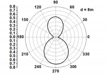
216      J. SUGANYA, J. A. BASKARADAS, U. SCIACCA, ET AL., SIMPLIFIED ANALYTICAL APPROACH FOR AN AIRBORNE BENT …

The log periodic V dipole antenna is analyzed as V dipole        ing environment and can be a very challenging issue to
in parallel connection [6] and its mutual coupling effects in    solve. The complication will become worse when the HF
[7].                                                             antenna hanging below the helicopter is used for the survey
      For an infinite zig zag antenna [8], derivation for the    of temperate glaciers. The structural stability of the HF
approximate expression of the phase velocity along with          wire antenna should be maintained throughout the airborne
the theoretical calculation for the radiation pattern and        flying time. Predicting the performance and validating the
characteristic impedance are discussed. For a single zig zag     procedure for an HF antenna below the helicopter is very
antenna, radiation properties and approximate expressions        difficult, acute with many difficulties.
for the radiation fields have been reported in [9]. Based on           The paper is organized as follows. The structure of
the radiated electric field by the elements of the yagi uda      the 10 MHz bent wire antenna [20] has been explained in
array, the far field analysis is done in [10]. The analytical    Sec. 2. Analytical equations for the radiated fields from the
field analysis of the yagi uda array uses the concept of         various segments of the wire antenna have been discussed
parasitic elements. In the order to maximize the forward         in Sec. 3. In that electric field equations for the vertical
gain in the yagi uda array, the optimum spacing between          segments, slant segments and horizontal segments of the
the elements is essential and a method of repeated applica-      wire have been derived separately. And also combined
tion of a perturbation procedure has been discussed in [11].     equation for the electric field due to active wire elements,
For short yagi aerials, the theoretical design data analysis     fields due to the parasitic wire elements of the GPR an-
has been discussed with different cases of driven and para-      tenna in the far field are provided in subsections with the
sitic elements placement in [12].                                final analytical equation for the total electric field of the
                                                                 considered 10 MHz GPR antenna system have been dis-
      For analyzing the bent wire antenna, we can consider
                                                                 cussed. In Sec. 4, with the help of simulation results, vali-
the thin linear antenna as a reference for deriving the far
                                                                 dation of the derived analytical equation using MATLAB
field components. Eighty years of progress in thin linear
                                                                 R2017b has been done with the numerical results of the
antenna have been given in detail in [13]. Without analyti-
                                                                 10 MHz antenna system using HFSS software. Section 5
cal equations, some papers have been reported in the past
                                                                 deals with the simulation results for the placement analysis
discussing the bent wire concepts in various aspects. The
                                                                 of the 10 MHz GPR antenna system hanging below the
effects on the rectangular spiral antenna have been ana-
                                                                 helicopter. This is used to find out the optimum range of
lyzed for its varying wire radius [14] and arm bent with the
                                                                 distances between the helicopter and the antenna system.
help of input impedance calculation. The effects of feed
                                                                 Finally, Section 6 is provided with the conclusion of this
wire on radiation characteristics are also discussed in [15].
                                                                 research paper.
The scattering and the radiation effects of the bent wire
having junctions are analyzed in [16]. Prediction about the
cross section of the bent wire is discussed in [17]. The field
equations in the time domain and the characterization of
                                                                 2. Structure of the Antenna
the antenna is done in [18]. Pattern synthesis of wire an-             The basic structure considered for modification in this
tenna in a simplified method of analysis for linear array        work is a thin wire dipole antenna. By altering the linear
elements has been described in [19].                             wire geometry, one can reduce or lower the resonant fre-
                                                                 quency of the whole antenna system, with acceptable
      Analytical equations in the above mentioned papers
                                                                 tradeoffs on the fundamental antenna parameters which
are only for the active bent antenna which is not having the
                                                                 decides the performance of the antenna. Here, the conven-
parasitic elements in their antenna system. For the yagi uda
                                                                 tional straight wire antenna is modified and bent to some
like structures, the driven, reflector, parasitic wires are
                                                                 angle for reducing the dimension of the antenna in its
straight without having the bents in them. In all the litera-
                                                                 length significantly. The main disadvantage that should be
ture papers reported so far, HF 10 MHz GPR bent wire
                                                                 compromised in the small size wire antennas are reduced
antenna having active, parasitic bent wires, with eight bent
                                                                 gain, low radiation efficiency and bandwidth. The better
angles in its structure have not been analyzed analytically
                                                                 way to reduce the dimension of the wire antenna is to in-
in terms of far field equations. In this work, a simplified
                                                                 troduce bends at appropriate lengths and angles for ob-
analysis of the 10 MHz antenna system theoretically, in
                                                                 taining better radiation efficiency and other antenna pa-
terms of far field equation has been discussed, which is the
                                                                 rameters. From the literature discussed so far, meander,
combination of linear wire elements, slant wire elements
                                                                 bowtie and zigzag type of wire antenna are found to be the
and parasitic wire elements. The 10 MHz bent wire an-
                                                                 better selection for the GPR application. But they cannot be
tenna’s [20] far field analytical equations for the electric
                                                                 used as it is, with their meander and zigzag shapes. The
field intensity are framed, simulated using MATLAB
                                                                 three main problems: radiation efficiency, bandwidth and
R2017b© and compared with the simulation results of the
                                                                 impedance matching should be considered while reducing
same antenna using HFSS© software. Plots of the calcu-
                                                                 the size of the antenna. The bending concept used in those
lated analytical result show good agreement with the sim-
                                                                 antenna can be utilized for forming new shapes and dimen-
ulation results obtained using the simulation software.
                                                                 sions for the 10 MHz frequency of operation with both
     The antenna hanging below the helicopter [21], [22]         transmitting and receiving antennas. The newly framed
will be influenced due to its interaction with the surround-     antenna should resonate at the required frequency with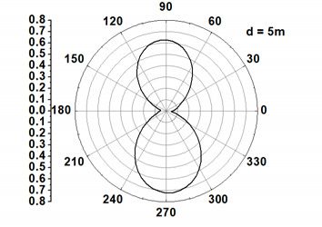
RADIOENGINEERING, VOL. 30, NO. 1, APRIL 2021                                                                              217

reduced dimension and acceptable performance character-
istics, when compared to the conventional straight dipole
wire antenna.
      The accurate characterization of the GPR antenna
system can be made with the help of the far field analytical
equations of the 10 MHz antenna. Analytical equations are
developed for the 10 MHz bent wire antenna in this paper.
Sinusoidal current distribution of the antenna structure with
zero currents at the ends is assumed. The considered
10 MHz wire antenna consists of transmitting and receiv-
ing wire elements. The transmitting wire structure alone of
the 10 MHz antenna system, can be decomposed into five
segments which are joined together as shown in the figure.
One vertical wire dipole, two (half) 45 degree slant wire
dipole and two (half) horizontal dipole joined together with
the structure shape specified as shown in Fig. 1 [20].
Symmetric segments are created in the receiving element as
well. The receiving wire unit will act as the parasitic ele-          Fig. 1. 10 MHz bent wire GPR antenna [20].
ment to the transmitting wire unit and the whole structure       is 1.6 for 10 MHz structure with the second bent at the
will resonate at 10 MHz. Without the parasitic wire ele-         ends of the first bent.
ment, the transmitting wire elements will not act as
an antenna for 10 MHz operating frequency. The total                   The antenna is designed using the copper wire. Dur-
length of the transmitting wire is 16.4 m. In which, ap-         ing the transmission, due to the fields around the driven
proximately 40% is the vertical wire segment, 20% is the         transmitting wire unit, the current is induced in the receiv-
slant wire dipole at each end of the vertical wire and 10%       ing parasitic element also. The 10 MHz bent wire dipole
of the total length of the transmitting wire is the horizontal   system is energized using a balanced transmission line.
wire dipole, at each end of the slant wires. T1, T2              Radiation from the transmission line is assumed to be zero
(T1 = T2 = 3.25 m), T3, T4 (T3 = T4 = 3.25 m), T5 & T6           here. The surrounding medium of the antenna system is air
(T5 = T6 = 1.7 m) are the six active segments in the trans-      here, as the antenna system is going to hang below the
mitting wire unit. The antenna wire thickness in terms of        helicopter. Method of analysis of the 10 MHz antenna is
radius is 0.0025 m and H = 2.3 m. The distance of separa-        same as that of the thin linear antenna. Current distribution
tion between the Tx and Rx units is D = 0.6 m. The bent          in both the transmitting and receiving (parasitic element
angle α is 45°. Same length and shape, as similar to that of     during transmission) wire units will have its influence in
transmitting segments, are there in the receiving wire unit      the far field region at point “P”. The current in the hori-
which will act as the parasitic elements during the trans-       zontal and in the slant segments are not getting vanished.
mission time of the GPR antenna system. The radius of the        The radiation pattern of the 10 MHz antenna is similar to
considered wire is very thin when compared to the overall        that of the normal dipole wire antenna.
length and the wavelength of the antenna unit. The 10 MHz             This 10 MHz antenna system is having the linear and
bent wire antenna structure [20] is as shown in Fig. 1. The      bent elements in both the driven and the parasitic elements
change in the shape of the linear wire antenna will have its     and also the whole system performance is not getting de-
influence in the impedance of the antenna and the radiation      graded due to the presence of the parasitic element. The
characteristics of the antenna system.                           change in the self-impedance and mutual impedance of the
      The inclusion of the two side bents in the linear active   antenna system depends on the total length of the wire
element and the presence of the identical parasitic element,     elements, type of the antenna material used, inclined angle
make the whole antenna system to resonate at 10 MHz              of the bent wire elements, distance of separation of the
frequency with the acceptable values of the antenna param-       wire segments and excitation feed type. Shift in the reso-
eters in the far field region. 6.5 m linear wire with the Tx     nant frequency and severe problems will be there for any
and Rx will not act as an antenna for 10 MHz, since the          antenna system placed in the real working environment.
reflection coefficient and the VSWR is very high. This bad       This is due to the interaction of the antenna system with its
S11 and VSWR values can be corrected by introducing one          surroundings with several unknown electrical, mechanical
bend at the ends of the linear existing wire at a slant angle    properties.
of 45 degrees. The expected 10 MHz resonant frequency                 GPR is the contactless method used to identify the
will be obtained after introducing the second bend at the        target using the antenna system in the glacier study. An-
ends of the first bend. The peak gain value with the 6.5 m       tenna plays the very important role which determines the
Tx linear element alone is 1.63. This decreases to 1.51          frequency of operation of the system and is the one which
peak gain value after the inclusion of Rx and first bent on      is having the direct interaction with the real environment.
either side of the linear element. Then the peak gain value      GPR antennas are more unique and different from the nor-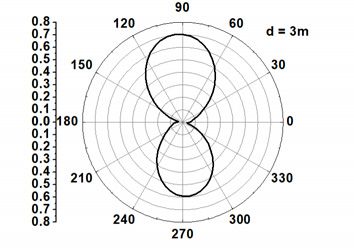
218 J. SUGANYA, J. A. BASKARADAS, U. SCIACCA, ET AL., SIMPLIFIED ANALYTICAL APPROACH FOR AN AIRBORNE BENT …
mal antennas, due to the application specific operating low frequency system setup. Melt water in voids, cavities
conditions. The needed features, performance specifica- and pockets in very less to large dimension levels may
tions, properties for the GPR system are required before cause the high frequency radar signal to scatter internally
designing the optimized antenna geometry for a specific within the ice layers and leads to the loss of signal some-
application. GPR configurations for different applications times. The internal scattering effects during the investiga-
enforce different constraints on antenna type and design to tion of the temperate glacier regions are greatly reduced
achieve high performance antennas as a result to obtain the with the usage of low frequency GPR systems at frequen-
clear subsurface image. The physical size of the antenna cies below about 10 MHz.
and the gain values are dependent quantity of the working
frequency. There should be some proper compromise in the
quantities such as gain, size and frequency of the antenna 3. Radiated Fields from the Segments
to achieve the GPR system compactness. The ultimate
consideration while designing the GPR antenna system is of the Wire Antenna
to have both transmitting and receiving elements within it In the analysis of the radiation from the considered
and with lower side lobes. This is helpful to avoid the bent wire antenna system, first we have to specify the cur-
power loss in the unwanted cross track direction during the rent in the active and parasitic source wire segments, then
survey time of the temperate glacier ice. the fields radiated by each segments. Electric and magnetic
Depending upon the measurement area conditions and vector potentials are the auxiliary functions which are used
the needed penetration depth in that specified survey area, as a mathematical tool for the analysis purpose to obtain
the GPR operating frequency band may range from few the electric field intensity E and magnetic field intensity H
MHz to a few GHz. The primary application of the low in the far field region of the considered antenna. The (x,y,z)
frequency - HF range (3 to 30 MHz) ground penetrating represents the observation point coordinates and (x’,y’,z’)
RADAR is to image the buried bedrock topography of the represents the source point coordinates. The whole evalua-
temperate glaciers. Narrow pulses will be used by the high tion of the existing fields in the far field region of the an-
frequency GPR for obtaining better resolution without tenna system depends on the most important actual current
deeper penetration. For deeper penetration, low frequency distribution quantity along each wire segments. The current
GPR systems are in need. The attenuation of the high fre- in the Tx and Rx segments are sinusoidal in nature with the
quency EM signal increases with the increase in the pene- maximum current value at the feeding position and zero
tration depth. So the high frequency signals are not able to value of current at the ends of the wire segments. The an-
penetrate much deeper into the surface layers for identify- tenna system is placed in the air medium. I0 is the maxi-
ing target such as bedrock. In this situation, we are in need mum amplitude of the assumed sinusoidal current distribu-
of a low frequency GPR system. tion.
Airborne survey, especially, helicopter borne GPR
survey will be more helpful to collect complex data safely 3.1 Tx Vertical Segments
and rapidly from large potentially high risk areas. An air-
borne survey can cover wider area, but deeper penetration T1, T2 are the vertical segments, oriented parallel to
is limited when compared to the ground based system. the Z axis of the coordinate system. In that, each vertical
Integrating the antenna system with the aircraft or helicop- and horizontal wires can be assumed as the vertically and
ter in an airborne system is a very important aspect to be horizontally placed linear antenna elements respectively.
considered seriously for doing the survey effectively. The ‘r’ is the distance from the origin of the coordinate system
suitable antenna frequency, relative positioning, placement, to the observation point ‘P’ in the far field region of the
orientation of the transmitting, receiving GPR antennas and antenna system. ‘R’ is the distance between the considered
appropriate transmitter power are vital, critical parameters antenna wire segments to the observation point under con-
for mapping the complex glacier bedrock. The weight of sideration. k 0 0 is the free space wave number. In
the antenna used for the airborne system should be reduced that, μ0 = 4π × 10–7 H/m is the permeability of free space
as much as possible. The weight of the antenna is the de- and ε0 = 8.85 × 10⁻¹² F/m is the permittivity of free space.
pendent quantity of its size. The size of the antenna is de- The overall length of the antenna for the transmitting sec-
termined by the operating frequency of the GPR system. tion is designated as ‘T’. Ivertical is the needed current distri-
bution in the vertical segment of the considered antenna
Existing temperate glacial survey area have difficul-
and is given by
ties and issues such as the varying electrical properties of
the dispersive, lossy, inhomogeneous, no-linear, aniso- I vertical ( x ' 0; y ' 0; z ')
tropic dielectric materials within the complex geometry
T T
glacial layers, irregular surface and subsurface, impose aˆz I 0 sin k 2 z ' ; 0 z' (1)
a difficult job in the modelling of the GPR antenna system. 5
Because of the presence of the combination of layers of aˆ I sin k T z ' ; T
ice, water, debris, rock, large sized stones, englacial chan- z 0 2 z' 0
5
nels in the temperate glacier regions, the GPR survey needs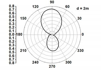
RADIOENGINEERING, VOL. 30, NO. 1, APRIL 2021 219
The finite length vertical wire antenna is subdivided into The finite length slant wire antenna is subdivided into
number of small infinitesimal dipoles of length ∆z׳. âz is the number small infinitesimal dipoles of length ∆z׳. For such
unit vector in Z axis direction. For such an infinitesimal a slant infinitesimal dipole inclined at an angle of 45° to the
dipole, the far field electric field component is given by Z axis, the far field electric field component is given by
j kI vertical ( x ', y ', z ') e jkR j kI slant ( x ', y ', z ') e jkR
dEθ(vertical) sin dz ' . (2) dEθ(slant) sin dz '. (6)
4 R 4 R cos
η is the intrinsic impedance of the air medium and is equal Integrating the Islant on the slant segment with respect to z '
to 120π. and applying limits which is confined only to the total slant
For obtaining the far electric field intensity due to the segment length will gives the Eθ(slant)
whole vertical segment of length 2T/5, we have to integrate 5T
dEθ with respect to the length along with the application of sin k T z ' e jkz 'cos dz '
far field approximations 2
2T
j I 0k e sin 5
jkr
0 T jkz 'cos Eθ(slant) 2T .
sin k z ' e dz ' 4 r cos 5
j I 0k e jkr sin 5
2 sin k T z ' e jkz 'cos dz '
T
Eθ(vertical) T . T 2
4 r 5 5
sin k T z ' e jkz 'cos dz '
0 2
(7)
After integrating and applying the limit which corresponds
(3) to the slant wire length will gives the Eθ(slant) and is given by
Integrating the current on the vertical segment with Eθ(slant)
respect to z ' and applying limits which is confined only to
3kT T
the vertical segment length will yields the Eθ(vertical) and is cos sin 10 sin k cos 5
given by
3kT T (8)
kT cos cos k cos
cos j I 0 e 10 5
jkr
.
2
jkr
2 r sin cos kT 2T
j I 0e 3T T (4) cos sin sin k cos
Eθ(vertical) cos sin sin k cos . 10 5
2 r sin 10 5
T cos kT cos k cos 2T
cos cos k cos
3T
10 5
10 5
The current continuity from the antenna wire feed po-
sition to the end of the wire is considered in the derivation
3.2 Tx Slant Segments which leads to the increase in the number of cosine and
The slant wire segments can also be considered as the sine terms in the derived equations. Bending the simple
antenna elements away from the origin which is inclined structure, linear half wavelength wire dipole antenna to
with an angle with respect to the reference axis. T3, T4 are some angle is one of the approaches used for reducing the
the slant wire segments which are inclined to 45° angle space occupied by the straight line wire antenna. The
with respect to the Z axis. Islant is the current in the slant length of the antenna and the size of the antenna is reduced
segment of the transmitting antenna system. Here the term by introducing various bents in the linear wire. Here in the
cosα has been included in the considered sinusoidal current 10 MHz wire antenna, such inclined bents are achieved
equation. Since the segment is forming an angle of α =45° with the slant segments placements at the ends of the linear
with the Z axis. The current is confined to the wire seg- wire elements on either side.
ments. So the direction of the current is same as that of the
orientation of the segments in the coordinate axis. The slant 3.3 Tx Horizontal Segments
segment current distribution is given by the following
equation T5, T6 are the horizontal wire segments, placed par-
allel to the Y axis. The current value becomes zero at the
I slant ( x ' 0; y ' 0; z ') ends of the horizontal segment. The below given current
I0 T T 2T equation (9) is for the one horizontal segment T5 for its
aˆ z cos sin k 2 z ' ; 5 z ' 5 (5) total length T/10,
I horizontal1 ( x ' 0; y '; z ' 0)
aˆ I0 T 2T T (9)
sin k z ' ; z' T 2T T
z cos 2 5 5 aˆ y I 0 sin k y ' ; y ' .
2 5 2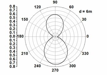
220 J. SUGANYA, J. A. BASKARADAS, U. SCIACCA, ET AL., SIMPLIFIED ANALYTICAL APPROACH FOR AN AIRBORNE BENT …
The finite length horizontal wire antenna is subdivided into the conventional wire dipole system, this 10 MHz antenna
number of small infinitesimal dipoles of length ∆y׳. ây is size is lesser. In order to reduce, limit the space occupied
the unit vector in Y axis direction. For such an infinitesi- by the 10 MHz antenna and to maintain the constant height
mal dipole which is parallel to the Y axis and placed in the of the whole system from the ground glacier surface,
YZ plane, the far field electric field component is given by bending the wire antenna laterally is done. The largest
dimension of this bent wire 10 MHz antenna is lesser than
j kI horizontal1 ( x ', y ', z ') e jkR the length of the conventional λ/2 dipole antenna. Bent
dEθ(horizontal1) cos sin dy '.
4 R wire 10 MHz dipole antenna is shorter than the straight
(10) wire dipole antenna used for the glaciological survey.
Integrating the Ihorizontal1 on the horizontal segment with If the length of the wire antenna increases, the induct-
respect to y ' and applying limits which is confined only to ance increases. Bending the linear wire will lead to the
the segment length will gives the Eθ(horizontal1) increase in the mutual capacitance between the adjacent
segments of the whole antenna system also. Here, the
Eθ(horizontal1)
bending is done laterally which increases the area occupied
T by the antenna system. Due to bending, there will be con-
j I 0k e jkr cos sin 2 T jky 'cos sistence in the decrement of the resonant frequency of the
sin k y ' e dy ' .
4 r 2T 2 wire with some variation in the inductance and capacitive
5 effects.
(11)
After integrating the current with respect to its length 3.5 Fields due to the Parasitic Wire Elements
and applying the limit which corresponds to the horizontal
wire length will yield the Eθ(horizontal1) and is given by While dealing with reduced size antenna system, the
mutual coupling effects will appear as an issue, which
j I 0 e jkr cos sin affects and degrades the actual working performance char-
Eθ(horizontal1)
4 r acteristics of the antenna. In this 10 MHz antenna system,
jk T2 cos both transmitter and receiver wire units will be there. The
e (12) distance of separation between them may not be half
sin 2 wavelength here. Why because, the wavelength for the
10 MHz frequency is 30 m. Half of the wavelength value
.
e jk 5 cos will be 15 m. We are unable to place the transmitter 15 m
2T
jcos sin kT cos kT apart from the receiver antenna. So, we have to go for the
10
2
sin 10 very minimal distance between them. In this situation, the
contribution of the receiving segments as a parasitic ele-
The above given equation is only for one Tx hori- ments, to the transmitting units will be there, due to strong
zontal segment. So, for the another horizontal segment, mutual coupling between them. As a whole, the antenna
same equation can be used as Eθ(horizontal2), since the place- system has to resonate at 10 MHz frequency.
ment of the T5, T6 segments is in the side of positive Y The distribution of current along the parasitic element
axis and integrating length limits for both the horizontal is similar to that of the current distribution in the active
segments are same. element. Since both the shape of the active Tx and parasitic
Rx are same. Due to this, the individual segments will have
its equal field composition in the far field region. During
3.4 Fields due to the Active Wire Elements the transmission of EM signal, even though we are
All the vertical, slant and horizontal wire segments of providing feed only to Tx section of the antenna system,
the transmitting and receiving units of the 10 MHz bent due to the mutual coupling of fields in between the driven
wire antenna are at equal distance from the ground. Be- bent elements and the parasitic structure, there will be
cause the bents are done laterally to the wire segments, all current flow in the parasitic element also. The electric field
the segments are in the same YZ plane. And also same side radiated by each segments of the antenna system are com-
lateral bending at both the ends of the transmitting wire bined together to produce the total field in the far field
antenna and also for the receiving wire antenna. The total region of the 10 MHz antenna system.
Eθ(active) (13) is the summation of the all the field which we In the GPR antenna system, both the Tx and the Rx
have derived individually for the segments and is given section wire should be there for transmitting the EM waves
below, through the Tx wires into the ice and receiving the re-
Eθ(active) Eθ(vertical) Eθ(slant) Eθ(horizontal1) Eθ(horizontal2) . (13) flected echoes with the help of the Rx wires. During the
transmission mode, the Rx will act as the parasitic element
The 10 MHz antenna should be placed below the for the driven active Tx wire and during the receiving
helicopter for glacier bedrock survey. When compared to mode the Tx bent wires will act as the parasitic element for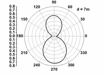
RADIOENGINEERING, VOL. 30, NO. 1, APRIL 2021 221
the receiving wire units. Both the wire sections are sepa- summation of field due to the active segments and the
rated by 0.6 m. Due to the mutual impedance in between parasitic segments and is given by
the driven and Rx bent wires, the current is induced in the
parasitic wire also. Since these two antenna wires are near Eθ(Total) Eθ(active) Eθ(parasitic) . (15)
to each other, some energy is getting coupled to the passive The total magnetic field intensity of the far field
wire from the active wire. The amount of energy getting component H∅(Total) can be calculated using the following
coupled to the parasitic element will depend on the current formula
distribution on the active wire element, radiation charac- E
teristics of the bent wires, separation of the Tx from the Rx H ( Total ) (Total ) . (16)
and the orientation of the various segment of wires in the
antenna system. There is a significant contribution of the The radiation efficiency decreases as the number of
parasitic wire segments to the driven wire segments, for bends increases in the active and parasitic element of the
resonating the whole antenna system at 10 MHz. Without antenna system. Modification in the dipole or monopole
the Rx wire segments, the Tx wire segments alone will not wire antenna will changes its physical and electrical char-
resonate at 10 MHz. The available power energy in the far acteristics to a greater extent. If the physical antenna size,
field region of the GPR antenna system depends not only shape are varied other than the linear structure the corre-
on the excited section but also the coupled excitation in the sponding changes in the impedance happen in the antenna
parasitic element. So, in the performance of the GPR an- system which will drastically change the antenna charac-
tenna system, the parasitic element plays an important role. teristics. Reduction in the physical size of the antenna will
The simplest way to find out the optimum distance reduce the antenna bandwidth to the greater extent.
between the elements is to increase the separation distance
from the minimum to the maximum acceptable range of
values. Through numerical simulation results, it has been 4. Simulation Results
confirmed that for the optimum separation of 0.6 m, the
antenna system parameters like return loss, VSWR, peak Plotting of the derived E(Total) analytical equation for
gain, Z parameter and the radiation efficiency are in the the 10 MHz bent wire GPR antenna system using
acceptable values. The degradation of the antenna system MATLAB R2017b is as shown in Fig. 2. If we consider the
performance in terms of resonating frequency and the an- 10 MHz antenna as a single straight wire, the total length
tenna parameters in the far field region should be kept in of the single wire will be 15 m. But in the case of ground
mind while finding out the optimum distance between the penetrating RADAR system, we are in need of two sepa-
active and passive element spacing. The optimum spacing rate antenna (one antenna for transmitting the electromag-
in between the Tx and Rx wires in this GPR antenna sys- netic signal and another one antenna for receiving the re-
tem is considered to be as 0.6 m, in order to operate the flected echo from the glaciers). Both the antenna should be
whole resonant system at 10 MHz. placed close to each other with more or less same radiation
characteristics and should be operated at the same fre-
Due to the 0.6 m separation between the active and quency but at different timings. If two straight wires of
the parasitic element of the antenna system, which is con- 15 m are used in which both the wires are separated by
sidered to be as minimum, when compared to the total some distance they will act as a bad radiator rather than the
length of the antenna, we can assume the maximum current good radiating antenna system.
in the parasitic wire also as I0. Substituting in the active
element E field equation will give us the field due to the
parasitic element in the far field region of the antenna sys-
tem. So, at the far field point ‘P’, the electric field intensity
Eθ(parasitic) due to the parasitic element is given by
Eθ(parasitic) E
θ(active) . (14)
3.6 Total Electric Field (Tx & Rx)
The total field of the GPR antenna system is the
summation of the fields from the individual linear hori-
zontal, vertical and slant antenna segments of the active
and parasitic wires. The radiation properties of the hori-
zontal, vertical and slanting wire are examined separately
and summed together at the last. The Er and E∅ are ap-
proximately equal to zero in the far field of the antenna Fig. 2. Plot of derived E(Total) analytical equation using
system. The approximate E(Total) - total electric field is the MATLAB.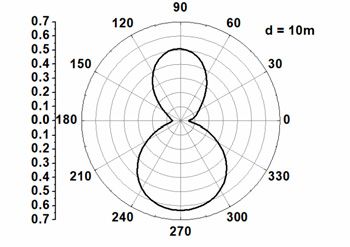
222       J. SUGANYA, J. A. BASKARADAS, U. SCIACCA, ET AL., SIMPLIFIED ANALYTICAL APPROACH FOR AN AIRBORNE BENT …

      The antennas will be at the same location and hence it         structures. Second, for the same bent wire antenna struc-
will create mutual coupling among themselves. This will              ture resonating at 10 MHz, the far electric field is plotted
consequently change, disturb the operating frequency and             using the HFSS (Finite Element Method) software (nu-
antenna parameters values. So considering all these issues           merical method for finding the field values). % Error =
in mind, this bent antenna is designed in the better way, to         [(Analytical value – Numerical value)/Analytical value]× 100.
operate at 10 MHz, as a whole system with eight bent an-             The estimated error between the analytical result (Equation
gles, including the transmitting & the receiving antenna             - MATLAB R2017b) and the numerical result (HFSS) is
units with vertical, slant and horizontal segments in it. So         26.4%. The analytical mathematical simulation result val-
now, it is easy for us to analyze the radiated fields sepa-          ues are considered as reference for calculating the esti-
rately for various segments of the antenna system and fi-            mated error. While deriving the analytical equation, we
nally add together to obtain needed analytical electric field        have considered the maximum current in the vertical, slant
equation at the far field.                                           and horizontal segments are the same as I0. This is not the
                                                                     actual situation prevailing in the bent antenna. The current
      The HFSS numerically simulated total electric field
                                                                     is maximum at the feed position and later on it starts de-
intensity result of the 10 MHz bent wire antenna is given in
                                                                     creasing towards its ends. That is, the maximum amplitude
Fig. 3. The current flow is getting continued at the bents of
                                                                     of the current will be maximum in the vertical segment and
the antenna structure, but it is not having zero value at the
                                                                     goes on decreasing in the slant and vertical segment. Be-
end of the vertical and also at the end of the slant segments.
                                                                     cause of that assumption there may be increase in the mag-
The current is getting vanished and become zero, only at
                                                                     nitude value of the electric field plotted using the equation
the end tip of the horizontal segments. This is the reason
                                                                     when compared to the numerical results and the estimated
that the analytical equation for the far field electric field
                                                                     error value will be 26.4%.
intensity is having many terms when compared to the nor-
mal linear antenna.                                                        Our interest in this paper is to obtain the far field -
                                                                     electric field intensity for the specified bent antenna struc-
      We have considered here that the radiation from the
                                                                     ture using both analytical and numerical analysis methods.
feed wire is having the minimum effect in the total radiated
                                                                     Due to the antenna structure complexity, only a few num-
field from the antenna system. The antenna is fed with the
                                                                     ber of practical antennas have been examined analytically.
uniform transmission line which is having the constant real
                                                                     It will be more effective to solve the electromagnetic field
characteristic impedance. The current distribution in the
                                                                     oriented problem of a wire antenna using analytical &
feed wire is not having much contribution to the field radi-
                                                                     numerical methods and proving the solutions in both the
ation by the antenna system is assumed here. With this we
                                                                     approaches are almost same. We tried in obtaining the far
have examined thoroughly only about the antenna system.
                                                                     field solutions using both the methods. The total electric
Because of the presence of the gap at the feed point of the
                                                                     field of the 10 MHz bent wire antenna has been obtained
antenna, there will be capacitance effect. The gap is fixed,
                                                                     using the HFSS (frequency domain solver) software which
small and hence the capacitance effect is almost constant
                                                                     are the numerical results. In HFSS, the electromagnetic
and negligible.
                                                                     fields around the antenna structure are solved using the
     In the paper, first, the electric field equation for the        finite element method. The 10 MHz whole antenna struc-
10 MHz bent wire antenna is derived (analytical way of               ture is divided into small volumes approximate meshes and
finding the far electric field values) and the derived final         the electric field is solved for the entire structure volume.
far electric field equation are simulated using MATLAB               In the meshes the Maxwell’s equations are solved. Auto-
R2017b software. The structure is having the vertical, slant         matic adaptive meshing is the most important part in the
and the horizontal segments in the active and parasitic wire         HFSS. With the help of the adaptive refinement process,
                                                                     the initial mesh created by the HFSS is refined. This pro-
                                                                     cess is continued till the result is converged and accurate.
                                                                     Normally numerical solutions are mostly valid for the
                                                                     specified mentioned frequency sweep and it follows the
                                                                     trial and error procedures to obtain the approximate solu-
                                                                     tions. But it handles the complex structure geometry shape
                                                                     very efficiently by forming the volume based mesh to find
                                                                     out the field solutions. Numerical method of analysis will
                                                                     provide an approximate solution whereas the analytical
                                                                     method of analysis will yield the exact solution results for
                                                                     the problem under consideration. The results we have
                                                                     obtained using the MATLAB software is the simulation of
                                                                     the analytical results (derived equation). Analytical theo-
                                                                     ries are more general, common approach and clear to un-
                                                                     derstand. Analytical solutions deal with the problem in the
      Fig. 3. Plot of total electric field of the 10 MHz bent wire
                                                                     well understood way of approach and are used to yield the
              antenna using HFSS.                                    exact solutions using the standard framed procedures. The
RADIOENGINEERING, VOL. 30, NO. 1, APRIL 2021 223
mathematical assumptions, rules of a wire antenna problem one. Considering the practical difficulties (both logistics
can be clearly understood in the analytical way of explain- and technical) in testing a low frequency airborne ground
ing the field solutions. In terms of accuracy, analytical penetrating radar antenna in the field, for optimizing the
solutions are better than the numerical solutions. Finding distance between the helicopter and antenna, the placement
a solution for the wire antenna related electromagnetic field issue has been simulated using a numerical analysis tool
problems in both analytical and simulation ways of ana- that gives very good approximation which will be close to
lysing methods will be stronger and acceptable. field experiment results. Here, the influence of the heli-
copter on the 10 MHz bent wire antenna is studied using
In the analytical way of analysing the far electric field
the EMPro© software. An optimized distance between the
of the 10 MHz bent wire antenna, the current distribution
helicopter and the antenna system is determined which will
of the antenna is specified first and then standard analysing
be then used for field measurements.
procedure is used to analyse the 10 MHz bent wire an-
tenna. If the diameter of the wire is less than 0.05λ, we can Figure 4 represents the scattering parameter (S11) and
assume the current distribution of the wire antenna as si- 2D radiation pattern of the 10 MHz bent wire antenna
nusoidal. As the frequency of operation of this antenna (without helicopter) simulated using EMPro©.
structure is 10 MHz, the corresponding wavelength value is
Figure 5 shows the arrangement of the helicopter and
30 meters. The 0.05λ is 1.5 meters for the 10 MHz fre-
the antenna during an airborne survey, which will be very
quency. But in our bent antenna design, the diameter of the
close to real time GPR survey. The helicopter considered
10 MHz bent antenna wire is 5 mm which is less than the
here is Eurocopter AS350 (CAD model from
0.05λ value. So in the analytical way of analysing the an-
https://grabcad.com/library/tag/helicopter) with the exact
tenna structure, the current distribution is considered to be
dimension. This is the model of the helicopter that is used
as sinusoidal. Using the intermediate auxiliary vector po-
by most of the GPR survey teams in Antarctica. The mate-
tentials, the field intensities are derived in the analytical
rial of the helicopter is considered to be a generic conduc-
approach for finding the field equations of the wire an-
tor/fiber as our interest is only to study the effect of the
tenna. The magnetic vector potential (A) and the electric
helicopter on the electromagnetic waves radiated from the
vector potential (E) are the auxiliary functions which are
antenna system.
found to be the important mathematical tools used to derive
the field intensity of an antenna in the far field region. The The S11 value versus frequency for the various dis-
electric and magnetic field intensities are the physically tance between the helicopter and the 10 MHz antenna sys-
measurable quantities for an antenna. The two step proce- tem have been plotted in Fig. 6. The distance (d) in be-
dure is followed (traditional way of solving wire antenna). tween the helicopter and the antenna is varied from 2 m to
First, the vector potentials are found out using the integra- 10 m and results have been plotted.
tion relations with the sources current densities J (electric
current source) and M (magnetic current source). Secondly,
the field intensities E, H are derived using the differentia-
tion of A and F. Proving the 10 MHz antenna structure
using the analytical equations can be contributed as
an added valid proof for the numerical results. Since the
10 MHz wire antenna structure is in bent shape and having
active and parasitic elements within it, the analytical solu-
tion for the far fields of this structure are not having simple
and less number of terms. Complex integration and the Fig. 4. S11 & 2D pattern of the 10 MHz antenna system
increased number of terms in the derived far field mathe- (without helicopter) in free space.
matical expression limits us to do the further derivation
expression for the power values, gain, and directivity.
5. Placement Analysis
The 10 MHz bent wire antenna considered in this
work has to be tested for its performance to find out the
optimum distance between the helicopter and the antenna
in the actual field to be surveyed before going for the final
deployment survey. In principle, the whole antenna should
be fabricated and tested in the field. Then appropriate
modifications are made in the distance between the heli-
copter and the antenna for improving and optimizing the
performance of the antenna system for the measurement
site. The whole process is time consuming and expensive Fig. 5. Placement of the antenna below the helicopter.224 J. SUGANYA, J. A. BASKARADAS, U. SCIACCA, ET AL., SIMPLIFIED ANALYTICAL APPROACH FOR AN AIRBORNE BENT …
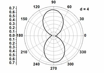
Fig. 6. S11 vs. frequency for various distance between the
helicopter and the antenna. Fig. 7. 2 D radiation pattern with varying helicopter-antenna
distances from 2 m to 10 m.
Distance d [m] Frequency [MHz] S11 [dB]
1 10.2 –3.9 and would act like a yagi reflector at a proper distance. So,
2 10.2 –5.1 flat conductor modeling of the helicopter is not appropri-
3 10.1 –6.7
ate. Above d = 4 m, the effect of the helicopter starts re-
4 10.1 –9.2
ducing and is evident from the 2D radiation patterns.
5 10.1 –12.2
6 10.1 –15.6 Comparing and analyzing the S11 and radiation plots,
7 10.1 –20.2 the distance from 7 m to 10 m are in the acceptable range
8 10.1 –27.6
for the real time survey. So we can choose the helicopter-
9 10.1 –40.7
10 10.1 –26.1
antenna distance in these range. The rope length of the
11 10.1 –21.3 antenna hanging below the helicopter is one of the critical
12 10.2 –22.6 component. An optimum rope length is done finally de-
13 10.2 –27.5 pending upon the selected glacier survey environment for
14 10.2 –40.2 avoiding unwanted ringing effects and blanking of glacier
Tab. 1. S11 vs frequency with varying helicopter-antenna
subsurface reflections. Suitable choice of the type of the
distance. helicopter, its speed and flight flying altitude above glacier
ground surface are also the essential things to be consid-
Table 1 lists the value of S11 at the resonant fre- ered for the survey. Here, with the help of the numerical
quency of the antenna system along with the helicopter for analysis software tool, the placement analysis simulations
various helicopter antenna distances from 1 m to 14 m. have been done and by examining the results obtained, the
From 1 m to 4 m distance of separation, the S11 values are optimum range of helicopter-antenna distances are deter-
greater than –10 dB which are not suggested for a good mined reducing test flight time which is expensive.
radiating system. The influence of the helicopter on the
radiation of the hanging antenna is more at these distances.
So these distances are not recommended for the real time
survey. Starting from the distance 5 m and greater than 6. Conclusion
that, the S11 is less than –10 dB which are the suitable A simplified procedure to analyze the far fields of
range of values. The antenna resonant frequency does not a 10 MHz bent wire antenna system is presented. The de-
vary that much from the required 10 MHz value. Lesser rived analytical equations of the electric field when plotted
value of S11 (–40.7 dB) is obtained at d = 9 m. is approximately having the same shape as that of the elec-
The 2D radiation pattern of the E field with varying tric field numerically simulated results of the whole an-
helicopter-antenna distance is given in Fig. 7. From these tenna structure. From this, it is evident that the modified
radiation patterns, it is evident that up to the distance of analytical equation holds well with the HFSS© simulation
d = 4 m, the influence of the helicopter is more. The results of the 10 MHz antenna system. The 10 MHz wire
proximity of the helicopter short-circuits the antenna, so antenna is having bents and parasitic influence for reso-
the radiation pattern cannot be so reliable which is well nating in its respective frequency. So, the presence of bents
observed with very poor S11 values. But the antenna pat- and parasitic element must be considered in deriving the
tern seems to be prominent above the helicopter. This can far field analytical equation for the antenna which is very
be due to the focusing effect of the diffracted radiowaves sensitive and influences the resonant frequency of the an-
from the irregular edges of the helicopter shape. If the tenna system. The optimum placement of the antenna be-
helicopter is considerd or modelled to be a flat conductor, low the helicopter during the GPR field survey must be
then it should reflect all the radiowaves from the antenna carefully chosen considering all the three antenna parame-RADIOENGINEERING, VOL. 30, NO. 1, APRIL 2021 225
ters: directivity, radiation pattern and S11 combined to- Radiolocation, 1946, vol. 93, no. 3, p. 598–614. DOI: 10.1049/ji-
3a-1.1946.0148
gether. The proposed analysis using a numerical simulation
tool is an efficient method to optimize the range of dis- [13] KING, R. W. P. The linear antenna-eighty years of progress.
tances between the low frequency antenna system and the Proceedings of the IEEE, 1967, vol. 55, no. 1, p. 2–16. DOI:
10.1109/PROC.1967.5373
helicopter used for the GPR field survey.
[14] NAKANO, H., YAMAUCHI, J., NOGAMI, K. Effects of wire
radius and arm bend on a rectangular spiral antenna. Electronics
Letters, 1983, vol. 19, no. 23, p. 957–958. DOI:
10.1049/el:19830651
Acknowledgments
[15] NAKANO, H., MINEGISHI, Y., HIROSE, K. Effects of feed wire
on radiation characteristics of a dual spiral antenna. Electronics
This work is carried out as part of Italian Antarctic Letters, 1988, vol. 24, no. 6, p. 363–364. DOI:
Research Activity (PNRA Program). The authors are 10.1049/el:19880246
thankful to the SASTRA – Keysight Center of Excellence [16] CHAO, H., STRAIT, B., TAYLOR, C. Radiation and scattering by
in RF System Engineering. configurations of bent wires with junctions. IEEE Transactions on
Antennas and Propagation, 1971, vol. 19, no. 5, p. 701–702. DOI:
10.1109/TAP.1971.1140021
[17] FANTE, R., HAZARD, K., DOLAN, J. RCS of bent wires. IEEE
References Transactions on Antennas and Propagation, 1968, vol. 16, no. 1,
p. 130–132. DOI: 10.1109/TAP.1968.1139098
[1] SCOTT BENNETT, W. A basic theorem that simplifies the [18] SHLIVINSKI, A., HEYMAN, E., KASTNER, R. Antenna
analysis of wire antennas. IEEE Antennas and Propagation characterization in the time domain. IEEE Transactions on
Magazine, 1998, vol. 40, no. 1, p. 22–30. DOI: 10.1109/74.667322 Antennas and Propagation, 1997, vol. 45, no. 7, p. 1140–1149.
[2] HAMID, M. A. K., BOERNER, W. M., SHAFAI, L., et al. DOI: 10.1109/8.596907
Radiation characteristics of bent-wire antennas. IEEE Transactions [19] SIAKAVARA, K., SAHALOS, J. N. A simplification of the
on Electromagnetic Compatibility, 1970, vol. 12, no. 3, synthesis of parallel wire antenna arrays. IEEE Transactions on
p. 106–111. DOI: 10.1109/TEMC.1970.303078 Antennas and Propagation, 1989, vol. 37, no. 7, p. 936–940. DOI:
[3] TSUKIJI, T., TOU, S. On polygonal loop antennas. IEEE 10.1109/8.29388
Transactions on Antennas and Propagation, 1980, vol. 28, no. 4, [20] SUGANYA, J., SCIACCA, U., BASKARADAS, J. A., et al.
p. 571–575. DOI: 10.1109/TAP.1980.1142380 Analysis of bent wire antenna resonant frequency for different bent
[4] EGASHIRA, S., TAGUCHI, M., SAKITANI, A. Consideration on angles. Radio Science, 2019, vol. 54, no. 12, p. 1240–1251. DOI:
the measurement of current distribution on bent wire antennas. 10.1029/2019RS006906
IEEE Transaction on Antennas and Propagation, 1988, vol. 36, [21] URBINI, S., CAFARELLA, L., TABACCO, I. E., et al. RES
no. 7, p. 918–926. DOI: 10.1109/8.7196 signatures of ice bottom near to Dome C (Antarctica). IEEE
[5] GOMEZ MARTIN, R., RUBIO BRETONES, A., FERNANDEZ Transactions on Geoscience and Remote Sensing, 2015, vol. 53,
PANTOJA, M. Radiation characteristics of thin-wire V-antennas no. 3, p. 1558–1564. DOI: 10.1109/TGRS.2014.2345457
excited by arbitrary time-dependent currents. IEEE Transactions [22] URBINI, S., ZIRIZZOTTI, A., BASKARADAS, J. A., et al.
on Antennas and Propagation, 2001, vol. 49, no. 12, Airborne Radio Echo Sounding (RES) measures on Alpine glaciers
p. 1877–1880. DOI: 10.1109/8.982473 to evaluate ice thickness and bedrock geometry: Preliminary
[6] CHAN, K. K., SILVESTER, P. Analysis of the log-periodic V- results from pilot tests performed in the Ortles Cevedale Group
dipole antenna. IEEE Transactions on Antennas and Propagation, (Italian Alps). Annals of Geophysics, 2017, vol. 60, no. 2, p. 1–12.
1975, vol. 23, no. 3, p. 397–401. DOI: DOI: 10.4401/ag-7122
10.1109/TAP.1975.1141070
[7] KYLE, R. Mutual coupling between log-periodic antennas. IEEE
Transactions on Antennas and Propagation, 1970, vol. 18, no. 1,
About the Authors...
p. 15–22. DOI: 10.1109/TAP.1970.1139613 SUGANYA Jayaraman was born in 1985. She received
[8] BHATNAGAR, P. S., SACHAN, S. B. L. Analysis of infinite zig- her BE degree in ECE from Arasu Engineering College
zag antenna. IEE-IERE Proceedings - India, 1976, vol. 14, no. 2, and ME degree in Communication Systems from Bannari
p. 44–46. DOI: 10.1049/iipi.1976.0015 Amman Institute of Technology, affiliated to Anna
[9] SENGUPTA, D. The radiation characteristics of a zig-zag antenna. University, Tamilnadu, India in 2006 and 2008
IRE Transactions on Antennas and Propagation, 1958, vol. 6, respectively. She worked in SRC, SASTRA Deemed
no. 2, p. 191–194. DOI: 10.1109/TAP.1958.1144571
University as Assistant Professor - II from 2008 to 2011.
[10] THIELE, G. A. Analysis of yagi-uda-type antennas. IEEE Currently, she is doing her full time PhD in SASTRA
Transactions on Antennas and Propagation, 1969, vol. 17, no. 1, Deemed to be University in the area of Radio Systems and
p. 24–31. DOI: 10.1109/TAP.1969.1139356
Antennas. Her research interests include electromagnetics,
[11] CHENG, D. K., CHEN, C. A. Optimum element spacings for antennas, microwave engineering.
Yagi-Uda arrays. IEEE Transactions on Antennas and
Propagation, 1973, vol. 21, no. 5, p. 615–623. DOI: James A. BASKARADAS (corresponding author)
10.1109/TAP.1973.1140551 received his PhD (2001) from Nagpur University, India.
[12] WALKINSHAW, W. Theoretical treatment of short Yagi aerials. He did his Post Doc. at the Istituto Nazionale Di Geofisica
Journal of the Institution of Electrical Engineers - Part IIIA: e Vulcanologia (INGV), Rome, Italy and continued as226 J. SUGANYA, J. A. BASKARADAS, U. SCIACCA, ET AL., SIMPLIFIED ANALYTICAL APPROACH FOR AN AIRBORNE BENT … Research Technologist at the same institute (2001 – 2014). Achille ZIRIZZOTTI received his Masters degree in His research interests are in radar instrumentation and Physics at "Sapienza" University of Rome in 1991 and remote sensing of ionosphere and glaciers. He has over 20 joined Istituto Nazionale di Geofisica e Vulcanologia publications and two patents. He participated in two Italian (INGV) in 1997. Now he is a Senior Research Technolo- Antarctic expeditions for radar remote sensing. At present gist at the INGV. Since 1997 he has been working on he is working as the Senior Assistant Professor at SASTRA glaciological radar as a Technologist at the INGV. The Deemed University, India. basic research interests are environmental geophysics, Umberto SCIACCA received his Masters. in Electronic glaciology, radar science in geophysics and glaciology. He Engineering at "Sapienza" University of Rome in 1989, was principal investigator and co-investigator of five Ital- following a remote sensing curriculum. He spent some ian Antarctic projects, developing Radio Echo Sounding years as a designer of electronic equipments in the space (RES) Systems widely used in Antarctica by the Italian industry. Now he is a Senior Technologist at Istituto Na- group and principal Coordinator of the Italian Radio Echo zionale di Geofisica e Vulcanologia, Rome (the Italian Sounding Database (IRES database). He participated in institution for Geophysics). His main activities include: eleven Antarctic expeditions from 1997 to 2015, collecting feasibility studies on the remote sensing electronic systems; over thirty thousand kilometers of radar data in various design, engineering and test of radar-based instrumentation projects (evaluation of the ice mass balance, determination to be used in geophysical applications (above all iono- of the drilling point of Epica project, Dome C ice condi- spheric sounders and radars for glacier prospecting). tions of the bedrock and subglacial lakes exploration).
You can also read