Towards Light-weight and Real-time Line Segment Detection
←
→
Page content transcription
If your browser does not render page correctly, please read the page content below
Towards Light-weight and Real-time Line Segment Detection

                                               Geonmo Gu*, Byungsoo Ko*, SeoungHyun Go, Sung-Hyun Lee, Jingeun Lee, Minchul Shin
                                                                             NAVER/LINE Vision
                                                                                    github.com/navervision/mlsd

                                                                       Abstract
arXiv:2106.00186v1 [cs.CV] 1 Jun 2021

                                           Previous deep learning-based line segment detection
                                        (LSD) suffer from the immense model size and high com-
                                        putational cost for line prediction. This constrains them
                                        from real-time inference on computationally restricted en-
                                        vironments. In this paper, we propose a real-time and light-
                                        weight line segment detector for resource-constrained en-
                                        vironments named Mobile LSD (M-LSD). We design an ex-
                                        tremely efficient LSD architecture by minimizing the back-
                                        bone network and removing the typical multi-module pro-
                                        cess for line prediction in previous methods. To maintain
                                        competitive performance with such a light-weight network,      Figure 1: Comparison of M-LSD and existing LSD methods
                                        we present novel training schemes: Segments of Line seg-       on Wireframe dataset. Inference speed (FPS) is computed
                                        ment (SoL) augmentation and geometric learning scheme.         on Tesla V100 GPU. Size and value of circles indicate the
                                        SoL augmentation splits a line segment into multiple sub-      number of model parameters (Millions). M-LSD achieves
                                        parts, which are used to provide auxiliary line data dur-      competitive performance with the lightest model size and
                                        ing the training process. Moreover, the geometric learning     the fastest inference speed. Details are in Table 3.
                                        scheme allows a model to capture additional geometric cues
                                        from matching loss, junction and line segmentation, length     vices, have made real-time line segment detection (LSD)
                                        and degree regression. Compared with TP-LSD-Lite, pre-         an essential but challenging task. The difficulty arises from
                                        viously the best real-time LSD method, our model (M-LSD-       the limited computational power and model size while find-
                                        tiny) achieves competitive performance with 2.5% of model      ing the best accuracy and resource-efficiency trade-offs to
                                        size and an increase of 130.5% in inference speed on GPU       achieve real-time inference.
                                        when evaluated with Wireframe and YorkUrban datasets.              With the advent of deep neural networks, deep learning-
                                        Furthermore, our model runs at 56.8 FPS and 48.6 FPS           based LSD architectures [30, 36, 31, 35, 12] have adopted
                                        on Android and iPhone mobile devices, respectively. To the     models to learn various geometric cues of line segments and
                                        best of our knowledge, this is the first real-time deep LSD    have proved to show improvements in performance. As de-
                                        method available on mobile devices.                            scribed in Figure 2, we have summarized multiple strategies
                                                                                                       that use deep learning models for LSD. The top-down strat-
                                                                                                       egy [30] first detects regions of line segment with attrac-
                                        1. Introduction                                                tion field maps and then predicts line segments by squeez-
                                           Line segments and junctions are crucial visual features     ing regions into line segments. In contrast, the bottom-
                                        in low-level vision, which provide fundamental informa-        up strategy first detects junctions, then arranges them into
                                        tion to the higher level vision tasks, such as pose estima-    line segments, and lastly verifies the line segments by us-
                                        tion [20, 29, 19], structure from motion [3, 18], 3D recon-    ing an extra classifier [36, 31, 35] or a merging algo-
                                        struction [5, 6], image matching [32], wireframe to image      rithm [10, 11]. Recently, [12] proposes Tri-Points (TP) rep-
                                        translation [33] and image rectification [34]. Moreover, the   resentation for a simpler process of line prediction without
                                        growing demand for performing such vision tasks on re-         the time-consuming steps of line proposal and verification.
                                        source constraint platforms, like mobile or embedded de-           Although previous efforts of using deep learning mod-
                                                                                                       els have made remarkable achievements, real-time infer-
                                          * Authors   contributed equally.                             ence for LSD on resource-constraint platforms still remains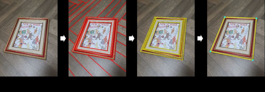
Stra-                              Inference speed (FPS)
                                                                                           Method         Input
                                                                                   tegy                           Backbone Prediction Total
                                                                                   TD      AFM            320       77.1       17.3   14.1
                                                                                           L-CNN          512       55.2      23.8     16.6
                                                                                   BU      L-CNN-P        512       55.2       0.4      0.4
                                                                                           HAWP           512       55.0      82.2     32.9
                                                                                           TP-LSD-Lite    320      138.4      234.6    87.1
                                                                                           TP-LSD-Res34   320      129.0       71.0    45.8
                                                                                    TP
                                                                                           TP-LSD-Res34   512      128.8       23.7    20.0
                                                                                           TP-LSD-HG      512       64.7      200.5    48.9
                                                                                           M-LSD-tiny     320      241.1     1202.8   200.8
                                                                                           M-LSD-tiny     512      201.6      881.9   164.1
                                                                                   Ours
                                                                                           M-LSD          320      156.3     1194.7   138.2
                                                                                           M-LSD          512      132.8      883.4   115.4

                                                                                  Table 1: Inference speed of backbone,
                                                                                  prediction modules, and total on GPU.
                                                                                  Strategies are from Figure 2. Our method
                                                                                  shows superior speed on backbone and
Figure 2: Different strategies for LSD. Previous LSD methods exploit the          line prediction by employing a light-
multi-module processing for line segment prediction. In contrast, our method      weight network with a single module of
directly predicts line segments from feature maps with a single module.           line prediction.

limited. There have been attempts to present real-time          smaller model size. M-LSD outperforms the previous best
LSD [12, 17, 31], but they have been limited to server-class    real-time method, TP-LSD-Lite [12], with only 6.3% of the
GPUs. This is mainly because the models that are used ex-       model size but gaining an increase of 32.5% in inference
ploit heavy backbone networks, such as dilated ResNet50-        speed. Moreover, M-LSD-tiny runs in real-time at 56.8 FPS
based FPN [35], stacked hourglass network [11, 17, 12],         and 48.6 FPS on Android and iPhone mobile devices, re-
and atrous residual U-net [30], which require large mem-        spectively. To the best of our knowledge, this is the first
ory and high computational power. In addition, as shown         real-time LSD method available on mobile devices.
in Figure 2, the line prediction process consists of multi-
ple modules, which include line proposal [30, 35, 36, 31],      2. Related Works
line verification networks [35, 36, 31] and mixture of con-
volution module [12, 11]. As the size of the model and the          Deep Line Segment Detection. There have been ac-
number of modules for line prediction increase, the over-       tive studies on deep learning-based LSD. In junction-based
all inference speed of LSD can become slower, as shown          methods, DWP [11] includes two parallel branches to pre-
in Table 1, while demanding higher computation. Thus,           dict line and junction heatmaps, followed by a merging
increases in computational cost make it difficult to deploy     process. PPGNet [35] and L-CNN [36] utilize junction-
LSD on resource-constraint platforms.                           based line segment representations with an extra classi-
    In this paper, we propose a real-time and light-weight      fier to verify whether a pair of points belongs to the same
line segment detector for resource-constrained environ-         line segment. Another approach exploits dense prediction.
ments, named Mobile LSD (M-LSD). For the network, we            AFM [30] predicts attraction field maps that contain 2-D
design a significantly efficient architecture with a single     projection vectors representing associated line segments,
module to predict line segments. By minimizing the net-         followed by a squeeze module to recover line segments.
work size and removing the multi-module process from            HAWP [31] is presented as a hybrid model of AFM and
previous methods, M-LSD is extremely light and fast. To         L-CNN. Recently, [12] devises the TP line representation
maintain competitive performance even with a light-weight       to remove the use of extra classifiers or heuristic post-
network, we present novel training schemes: SoL augmen-         processing from previous methods and proposes TP-LSD
tation and geometric learning scheme. SoL augmentation          network with two branches: TP extraction and line segmen-
divides a line segment into subparts, which are further used    tation branches. However, previous multi-module process-
to provide augmented line data during the training phase.       ing for line prediction, such as line verification network,
Geometric learning schemes train a model with additional        squeeze module, and multi-branch network can limit for
geometric information, including matching loss, junction        real-time inference on resource-constrained environments.
and line segmentation, length and degree regression. As a           Real-time Object Detectors. Real-time object detec-
result, our model is able to capture extra geometric informa-   tion has been an important task for deep learning-based ob-
tion during training to make more accurate line predictions.    ject detection. Object detectors proposed in the early days,
    As shown in Figure 1, our methods achieve competitive       such as RCNN-series [8, 7, 24] consist of two-stage archi-
performance and faster inference speed with an extremely        tecture: generating proposals in the first stage, then classi-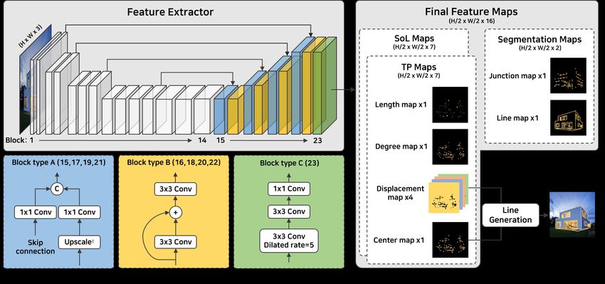
Figure 3: The overall architecture of M-LSD-tiny. In the feature extractor, block 1 ∼ 11 are parts of MobileNetV2, and
 block 12 ∼ 16 are designed as a top-down architecture. The final feature maps are simply generated by upscale. The
 predicted line segments are generated by merging center points and displacement vectors from the TP maps.

fying the proposals in the second stage. These two-stage de-    to build a light-weight LSD model, our encoder networks
tectors typically suffer from slow inference speed and hard     are based on MobileNetV2 [25] which is well-known to run
optimization difficulty. To handle this problem, one-stage      in real-time on mobile environments. The encoder network
detectors, such as YOLO-series [21, 22, 23] and SSD [15]        uses parts of MobileNetV2 (block 1 ∼ 11 of the feature ex-
are proposed to achieve GPU real-time inference by reduc-       tractor in Figure 3) to make it even lighter, which includes
ing backbone size and simplifying the two-stage process         an input to 64-channel of bottleneck blocks. The number of
into a one-stage process. This one-stage architecture has       parameters in the encoder network is 0.25M (7.4% of Mo-
been further studied and improved to run in real-time on        bileNetV2) while the total parameters of MobileNetV2 are
mobile devices [9, 25, 28, 14]. Motivated by the transi-        3.4M. For M-LSD, a slightly bigger yet more performant
tion from two-stage to one-stage architecture in object de-     model, the encoder network also uses parts of MobileNetV2
tection, we argue that the complicated multi-module pro-        including an input to 96-channel of bottleneck blocks which
cessing in previous LSD can be disregarded. We simplify         results to a number of 0.56M parameters (16.5% of Mo-
the line prediction process with a single module for faster     bileNetV2). The decoder network is designed using a com-
inference speed and enhance the performance by the effi-        bination of block types A, B, and C. Block type A con-
cient training strategies; SoL augmentation and geometric       catenates feature maps from skip connection and upscale.
learning scheme.                                                Block type B performs two 3 × 3 convolutions with a resid-
                                                                ual connection in-between. Similarly, block type C per-
3. M-LSD for Line Segment Detection                             forms two 3 × 3 convolutions followed by a 1 × 1 con-
                                                                volution, where the first is a dilated convolution. The fi-
    In this section, we present the details of M-LSD. Our de-   nal feature maps in M-LSD-tiny are generated by upscal-
sign mainly focuses on efficiency while retaining compet-       ing with H/2 × W/2 × 16 tensors when the input image is
itive performance. Firstly, we design a light-weight back-      H × W × 3. On the other hand, M-LSD uses the feature
bone and reduce the modules involved in processing line         map from block type C as a final feature map with the same
predictions for better efficiency. Next, we apply additional    size of H/2 × W/2 × 16.
training schemes, including SoL augmentation and geomet-
                                                                   Each feature map channel serves its own purpose: 1) TP
ric learning schemes, to capture extra geometric cues. As a
                                                                maps have seven feature maps, including one length map,
result, M-LSD is able to balance the trade-off between ac-
                                                                one degree map, one center map, and four displacement
curacy and efficiency to be well suited for mobile devices.
                                                                maps. 2) SoL maps have seven feature maps with the same
                                                                configuration as TP maps. 3) Segmentation maps have two
3.1. Light-weight Backbone
                                                                feature maps, including junction and line maps. Please re-
  We design light (M-LSD) and lighter (M-LSD-tiny)              fer to the supplementary material for further details on the
models as popular encoder-decoder architectures. In efforts     architectures of M-LSD-tiny and M-LSD.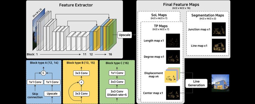
ever, we observe that the number of positive (foreground)
                                                                      pixels is much less than that of negative (background) pix-
                                                                      els, and such foreground-background class imbalance de-
                                                                      grades the performance of the WBCE loss. This is because
                                                                      the majority of pixels are easy negatives that contribute no
                                                                      useful learning signals. Thus, we separate positive and neg-
                                                                      ative terms of the binary cross-entropy loss to have the same
                                                                      scale, and reformulate a separated binary classification loss
     (a) TP representation               (b) SoL augmentation         as follows:
                                                                                                       P
Figure 4: Tri-Points (TP) representation and Segments of                          `pos (F ) = P −1I(p)  p W (p) · logσ(F (p)), (2)
Line segment (SoL) augmentation. ls , lc , and le denote
                                                                                                    p
                                                                                                P
start, center, and end points, respectively. ds and de are dis-       `neg (F ) =   P −1
                                                                                                  p (1   − I(p)) · log(1 − σ(F (p))),      (3)
                                                                                     p 1−I(p)

placement vectors to start and end points. l0 ∼ l2 indicates                        `cls (F ) = λpos · `pos (F ) + λneg · `neg (F ), (4)
internally dividing points of the line segment ls le .
                                                                      where I(p) outputs 1 if the pixel p of the GT map is non-
                                                                      zero, otherwise 0, σ denotes a sigmoid function, and W (p)
3.2. Line Segment Representation                                      and F (p) are pixel values in the GT and feature map, re-
                                                                      spectively. We use the center loss as Lcenter = `cls (C),
    Line segment representation determines how line seg-
                                                                      where C denotes center map and set the weights (λpos ,
ment predictions are generated and ultimately affects the
                                                                      λneg ) as (1,30). For the displacement loss Ldisp , we use
efficiency of LSD. Hence, we employ the TP representa-
                                                                      smooth L1 loss for regression learning as [12].
tion [12] which has been introduced to have a simple line
generation process and shown to perform real-time LSD us-             3.3. SoL Augmentation
ing GPUs. TP representation uses three key-points to depict
a line segment: start, center, and end points. As illustrated             We propose Segments of Line segment (SoL) augmenta-
in Figure 4a, the start ls and end le points are represented          tion that increases the number of line segments with wider
by using two displacement vectors (ds , de ) with respect to          varieties of length for training. Learning line segments with
the center lc point. The line generation process, which is to         center points and displacement vectors can be insufficient in
convert center point and displacement vectors to a vector-            certain circumstances where a line segment may be too long
ized line segment, is performed as:                                   to manage within the receptive field size or the center points
                                                                      of two distinct line segments are too close to each other. To
         (xls , yls ) = (xlc , ylc ) + ds (xlc , ylc ),               address these issues and provide auxiliary information to
         (xle , yle ) = (xlc , ylc ) + de (xlc , ylc ),         (1)   the TP representation, SoL explicitly splits line segments
                                                                      into multiple subparts with overlapping portions with each
where (xα , yα ) denotes the α point. ds (xlc , ylc ) and             other. An overlap between each split is enforced to preserve
de (xlc , ylc ) indicate 2D displacements from the center point       connectivity among the subparts. As described in Figure 4b,
lc to the corresponding start ls and end le points. The center        we compute k internally dividing points (l0 , l1 , l2 ) and sepa-
point and displacement vectors are trained with one cen-              rate the line segment ls le into three subparts (ls l1 , l0 l2 , l1 le ).
ter map and four displacement maps (one for each x and                Expressed in TP representation, each subpart is trained as if
y value of the displacement vectors ds and de ). For the              it is a typical line segment. The number of internally divid-
ground truth (GT) of the center map, positions of the center          ing points k is determined by the length of the line segment
point are marked on a zero map, which is then scaled using            as k = br(l)/(µ/2)e − 1, where r(l) denotes the length of
a Gaussian kernel truncated by a 3 × 3 window. In the line            line segment l, and µ is the base length of subparts. Note
generation process, we extract the exact center point posi-           that when k ≤ 1, we do not split the line segment. The re-
tion by non-maximum suppression on the center map. Next,              sulting length of each subpart can be shorter or longer than
we generate line segments with the extracted center points            µ, and we use µ = input size × 0.125. Loss functions
and the corresponding displacement vectors using a sim-               Lcenter and Ldisp for SoL maps are the same as Equation 4
ple arithmetic operation as expressed in Equation 1; thus,            and smooth L1 loss, respectively, when the ground truth is
making inference efficient and fast. For a direct comparison          from subparts. Note that the line generation process is only
with [12], we perform the line generation immediately from            done in TP maps, not in SoL maps.
the final feature maps in a single module process, while [12]
                                                                      3.4. Learning with Geometric Information
performs multi-module processing as illustrated in Figure 2.
    For a loss function to train the center map, the weighted            To boost the quality of predictions, we incorporate vari-
binary cross-entropy (WBCE) loss is used in [12]. How-                ous geometric information about line segments which helps
3.4.2   Junction and Line Segmentation
                                                                      Center point and displacement vectors are highly related to
                                                                      pixel-wise junctions and line segments in the segmentation
                                                                      maps of Figure 3. For example, end points, derived from
                                                                      the center point and displacement vectors, should be the
                                                                      junction points. Also, center points must be localized on
                                                                      the pixel-wise line segment. Thus, learning the segmenta-
        (a) Matching loss                (b) Geometric losses         tion maps of junctions and line segments works as a spatial
                                                                      attention cue for LSD. As illustrated in Figure 3, M-LSD
Figure 5: Matching and geometric losses. (a) Given a
                                                                      contains segmentation maps, including a junction map and
matched pair of a predicted line ˆl and a GT line l, matching
                                                                      a line map. We construct the junction GT map by scaling
loss (Lmatch ) optimizes the predicted start, end, and cen-
                                                                      with Gaussian kernel as the center map, while using a bi-
ter points. (b) Given a line segment, M-LSD learns various
                                                                      nary map for line GT map. The separated binary classifica-
geometric cues: junction (Ljunc ) and line (Lline ) segmen-
                                                                      tion loss is used for the junction loss Ljunc = `cls (J) and
tation, length (Llength ) and degree (Ldegree ) regression.
                                                                      line loss Lline = `cls (E), where J and E denote junction
the overall learning process. In this section, we present             and line maps, respectively. The total segmentation loss is
learning LSD with matching loss, junction and line segmen-            defined as Lseg = Ljunc + Lline , where we set the weights
tation, and length and degree regression for additional geo-          (λpos , λneg ) as (1, 30) for Ljunc and (1, 1) for Lline .
metric information.
                                                                      3.4.3   Length and Degree Regression
3.4.1   Matching Loss
                                                                      As displacement vectors can be derived from the length and
Line segments under the TP representation are decoupled               degree of line segments, they can be additional geometric
into center points and displacement vectors, which are op-            cues to support the displacement maps. We compute the
timized with center and displacement loss separately. They            length and degree from the ground truth and mark the values
become line segments by the line generation process as for-           on the center of line segments in each GT map. Then, these
mulated in Equation 1. However, this coupled informa-                 values are extrapolated to a 3 × 3 window so that all neigh-
tion of the generated line segment is under-utilized in loss          boring pixels of a given pixel contain the same value. As
functions. Thus, we present a matching loss, which also               shown in Figure 3, we maintain predicted length and degree
leverages information of the coupled information w.r.t the            maps for both TP and SoL maps, where TP uses the origi-
ground truth. Note that matching loss is used for both TP             nal line segment and SoL uses augmented subparts. As the
and SoL maps.                                                         ranges of length and degree are wide, we divide each length
    As illustrated in Figure 5a, matching loss guides the gen-        by the diagonal length of the input image for normalization.
erated line segments to be similar to the matched GT. We              For degree, we divide each degree by 2π and add 0.5. Fi-
first take the endpoints of each prediction, which can be             nally, the length and degree maps are used for smooth L1
calculated via the line generation process, and measure the           loss (Llength and Ldegree ) based regression learning.
Euclidean distance d(·) to the endpoints of the GT. Next,
these distances are used to match predicted line segments ˆl          3.5. Final Loss Functions
with GT line segments l that are under a threshold γ:                    The loss function for TP maps LT P is defined as the sum
             d(ls , ˆls ) < γ and d(le , ˆle ) < γ,             (5)   of center and displacement loss, length and degree regres-
                                                                      sion loss, and a matching loss:
where ls and le are the start and end points of the line l, and
γ is set to 5 pixels. Then, we obtain a set M of matched line         LT P = Lcenter + Ldisp + Llength + Ldegree + Lmatch . (7)
segments (l, ˆl) that satisfies this condition. Finally, the L1
loss is used for the matching loss, which aims to minimize            The loss function for SoL maps LSoL follows the same for-
the geometric distance of the matched line segments w.r.t             mulation as Equation 7 but with SoL augmented GT. Fi-
the start, end, and center points as follows:                         nally, we obtain the final loss function Ltotal as follows:
                     1     X
  Lmatch =                       k ls − ˆls k1 + k le − ˆle k1                    Ltotal   = LT P + LSoL + Lseg .              (8)
                   |M|
                            (l,l̂)∈M

                   + k C̃(ˆl) − (ls + le )/2 k1 ,               (6)   As illustrated in Figure 3, LT P and LSoL each optimizes
                                                                      the line representation maps and Lseg optimizes the seg-
where C̃(ˆl) is center point of a line ˆl from the center map.        mentation maps.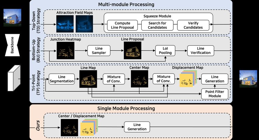
(a) w/o matching loss (M2)     (b) w/ matching loss (M3)         (a) Junction segmentation map       (b) Line segmentation map

(c) w/o SoL augmentation (M7) (d) w/ SoL augmentation (M8)          (c) TP length regression map    (d) TP degree regression map
Figure 6: Saliency maps generated from TP center map.              Figure 7: Saliency maps generated from each feature map.
Model numbers (M2∼8) are from Table 2.                             M-LSD-tiny (M8 in Table 2) model is used for generation.

4. Experiments                                                            M   Schemes                    FH     sAP 10   LAP
                                                                          1   Baseline                   73.2    47.6    46.8
4.1. Experimental Setting                                                 2   + Input augmentation       74.3    48.9    48.1
                                                                          3   + Matching loss            75.4    52.2    52.5
    Dataset and Evaluation Metrics.          We evaluate our              4   + Line segmentation        75.4    52.9    53.7
model with two famous LSD datasets: Wireframe [11] and                    5   + Junction segmentation    76.2    53.7    54.6
YorkUrban [5]. The Wireframe dataset consists of 5,000                    6   + Length regression        76.1    54.5    54.8
                                                                          7   + Degree regression        76.2    55.1    55.3
training and 462 test images of indoor and outdoor scenes,
                                                                          8   + SoL augmentation         77.2    58.0    57.9
while the YorkUrban dataset has 102 test images. Follow-
ing the typical training and test protocol [12, 35, 17, 30, 36],   Table 2: Ablation study of M-LSD-tiny on Wireframe. The
we train our model with the training set from the Wire-            baseline is trained with M-LSD-tiny backbone including
frame dataset and test with both Wireframe and YorkUr-             only TP representation. M denotes model number.
ban datasets. We evaluate our models using prevalent met-
rics for LSD [12, 35, 17, 30, 36] that include: heatmap-           which is generated from each feature map to analyze the
based metric F H , structural average precision (sAP), and         network learned from each training scheme. The saliency
line matching average precision (LAP).                             map interprets important regions and importance levels on
    Optimization. We train our model on Tesla V100 GPU.            the input image by computing the gradients from each fea-
We use the TensorFlow [2] framework for model training             ture map. We include a comparison of models in Figure 6
and TFLite [1] for porting models to mobile devices. In-           and feature maps in Figure 7.
put images are resized to 320 × 320 or 512 × 512 in both               Baseline and Augmentation. The baseline model is
training and testing, which are specified in each experiment.      trained with M-LSD-tiny backbone, including only the TP
The input augmentation consists of horizontal and vertical         representation and no other proposed schemes. We observe
flips, shearing, rotation, and scaling. We use ImageNet [4]        that adding horizontal and vertical flips, shearing, rota-
pre-trained weights on the parts of MobileNetV2 [25] in M-         tion, and scaling input augmentation on the baseline model
LSD and M-LSD-tiny. Our model is trained using the Adam            shows further performance improvement.
optimizer [13] with a learning rate of 0.01. We use linear             Matching Loss. Integrating matching loss shows slight
learning rate warm-up for 5 epochs and cosine learning rate        improvements on pixel localization accuracy by 1.1 in F H
decay [16] from 70 epoch to 150 epoch. We train the model          while significant enhancements on line prediction quality
for a total of 150 epochs with a batch size of 64.                 by 3.3 in sAP 10 and 4.4 in LAP . We observe from saliency
                                                                   maps that learning w/o matching loss shows weak attention
4.2. Ablation Study and Interpretability
                                                                   on center points, as shown in Figure 6a, while w/ matching
   We conduct a series of ablation experiments to analyze          loss amplifies the attention on center points in Figure 6b.
our proposed method. M-LSD-tiny is trained and tested on           This demonstrates that training with coupled information of
the Wireframe dataset with an input size of 512 × 512. As          center points and displacement vectors allows the model to
shown in Table 2, all the proposed schemes contribute to a         learn with more line-awareness features.
significant performance improvement. In addition, we in-               Line and Junction Segmentation. Adding line and
clude saliency map visualizations by using GradCam [26],           junction segmentation gives performance boosts in the fol-
Wireframe                      YorkUrban
              Methods             Input                                                              Params(M)    FPS
                                          FH     sAP5 sAP10      LAP      FH    sAP5 sAP10    LAP
              LSD [27]             320    64.1    6.7    8.8     18.7    60.6    7.5   9.2    16.1       -       100.0†
              DWP [11]             512    72.7     -     5.1      6.6    65.2     -     2.6    3.1      33.0       2.2
              AFM [30]             320    77.3   18.3   23.9     36.7    66.3    7.0   9.1    17.5      43.0      14.1
              L-CNN [36]           512    77.5   58.9   62.8     59.8    64.6   25.9   28.2   32.0      9.8       16.6
              L-CNN-P [36]         512    81.7   52.4   57.3     57.9    67.5   20.9   23.1   26.8      9.8        0.4
              LGNN [17]            512     -       -    62.3       -      -       -      -      -        -        15.8‡
              LGNN-lite [17]       512     -       -    57.6       -      -       -      -      -        -        34.0‡
              HAWP [31]            512    80.3   62.5   66.5     62.9    64.8   26.1   28.5   30.4      10.4      32.9
              TP-LSD-Lite [12]     320    80.4   56.4   59.7     59.7    68.1   24.8   26.8   31.2      23.9      87.1
              TP-LSD-Res34 [12]    320    81.6   57.5   60.6     60.6    67.4   25.3   27.4   31.1      23.9      45.8
              TP-LSD-Res34 [12]    512    80.6   57.6   57.2     61.3    67.2   27.6   27.7   34.3      23.9      20.0
              TP-LSD-HG [12]       512    82.0   50.9   57.0     55.1    67.3   18.9   22.0   24.6      7.4       48.9
              M-LSD-tiny           320    76.8   43.0   51.3     50.1    61.9   17.4   21.3   23.7      0.6      200.8
              M-LSD-tiny           512    77.2   52.3   58.0     57.9    62.4   22.1   25.0   28.3      0.6      164.1
              M-LSD                320    78.7   48.2   55.5     55.7    63.4   20.2   23.9   27.7      1.5      138.2
              M-LSD                512    80.0   56.4   62.1     61.5    64.2   24.6   27.3   30.7      1.5      115.4

Table 3: Quantitative comparisons with existing LSD methods. FPS is evaluated in Tesla V100 GPU, where † denotes CPU
FPS and ‡ denotes the value from the corresponding paper because of no published implementation. The best score from
previous methods and our models are colored in blue and red, respectively.

lowing metrics: 0.8 in F H , 1.5 in sAP 10 and 2.1 in LAP .             TP-LSD [12]. Table 3 shows that our method achieves com-
Moreover, the junction and line attention on saliency maps              petitive performance and the fastest inference speed even
of Figure 7a and 7b are precise, which shows that junction              with a limited model size. In comparison with the previous
and line segmentations work as spatial attention cues for               fastest model, TP-LSD-Lite, M-LSD with input size of 512
LSD.                                                                    shows higher performance and an increase of 32.5% in in-
    Length and Degree Regression. The line prediction                   ference speed with only 6.3% of the model size. Our fastest
quality improves 1.4 in sAP 10 and 0.7 in LAP by adding                 model, M-LSD-tiny with 320 input size, has a slightly lower
length and degree regression, while the pixel localization              performance than that of TP-LSD-Lite, but achieves an in-
accuracy F H remains the same. The length saliency map in               crease of 130.5% in inference speed with only 2.5% of
Figure 7c contains highlights on the entire line, and the de-           the model size. Compared to the previous lightest model
gree saliency map in Figure 7d has highlights on the center             TP-LSD-HG, M-LSD with 512 input size outperforms on
points. We speculate that computing length needs the entire             sAP 5 , sAP 10 and LAP with an increase of 136.0% in in-
line information whereas computing the degree only needs                ference speed with 20.3% of the model size. Our lightest
part of the line. Overall, learning with additional geomet-             model, M-LSD-tiny with 320 input size, shows an increase
ric information of line segments, such as length and degree,            of 310.6% in the inference speed with 8.1% of the model
further increases the performance.                                      size compared to TP-LSD-HG. Previous methods can be
    SoL Augmentation.         Integrating SoL augmentation              deployed as real-time line segment detectors on server-class
shows significant performance boost by 1.0 in F H , 2.9 in              GPUs, but not on resource-constrained environments either
sAP 10 and 2.6 in LAP . In the saliency maps of Figure 6c               because the model size is too large or the inference speed
and 6d, w/o SoL augmentation shows strong but vague at-                 is too slow. Although M-LSD does not achieve state-of-
tention on center points with disconnected line attention for           the-art performance, it shows competitive performance and
the long line segments, when the entire line information is             the fastest inference speed with the smallest model size, of-
essential to compute the center point. However, w/ SoL                  fering the potential to be used in real-time applications on
augmentation shows more precise center point attention as               resource-constrained environments, such as mobile devices.
well as clearly connected line attention. It demonstrates that
augmenting line segments based on the number and length                 4.4. Visualization
guides the model to be more robust in pixel-based and line                 We visualize outputs of M-LSD and M-LSD-tiny in Fig-
matching-based qualities.                                               ure 8. Junctions and line segments are colored with cyan
                                                                        blue and orange, respectively. Compared to the GT, both
4.3. Comparison with Other Methods
                                                                        models are capable of identifying junctions and line seg-
   We compare our method with previous LSD methods, in-                 ments with high precision even in complicated low con-
cluding LSD [27], DWP [11], AFM [30], L-CNN [36] with                   trast environments such as (a) and (c). Although M-LSD-
post-processing (L-CNN-P), LGNN [17], HAWP [31], and                    tiny contains a few missing small line segments and incor-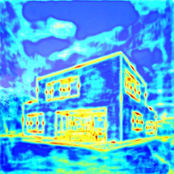
Model Input Device FP Latency (ms) FPS Memory (MB)
32 30.6 32.7 169
iPhone
16 20.6 48.6 111
320
32 31.0 32.3 103
Android
16 17.6 56.8 78
M-LSD-tiny
32 51.6 19.4 203
iPhone
16 36.8 27.1 176
512
32 55.8 17.9 195
Android
16 25.4 39.4 129
32 74.5 13.4 241
iPhone
16 46.4 21.6 188
320
32 82.4 12.1 236
Android
16 38.4 26.0 152
M-LSD
32 121.6 8.2 327
iPhone
16 90.7 11.0 261
512
32 177.3 5.6 508
Android
16 79.0 12.7 289
Table 4: Inference speed and memory usage on iPhone
(A14 Bionic chipset) and Android phone (Snapdragon 865
Figure 8: Qualitative evaluation of M-LSD-tiny and M-LSD chipset). FP denotes floating point.
on WireFrame dataset.
rectly connected junctions, the fundamental line segments
to aware of the environmental structure are accurate. In ad-
dition, there are straight patterns on the floor in (b) and the
wall in (d), that are missing in GT taken from the Wire-
Frame [11] dataset which was annotated by humans. How-
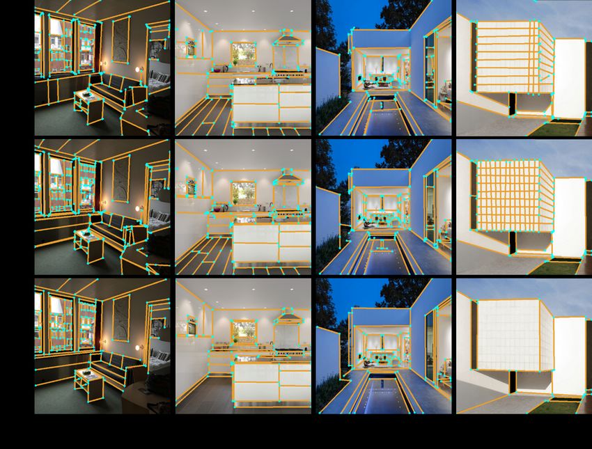
ever, our proposed methods are capable of detecting even Figure 9: Real-time box detection using M-LSD-tiny on a
the minute details in patterns and confirms the robustness mobile device. Given an image as input to the mobile device
of our models against complicated scenes. as (a), line segments are detected using M-LSD-tiny as (b).
Then, box candidates are computed from post-processing as
4.5. Deployment on Mobile Devices (c), and finally we obtain box detection by a ranking process
We deploy M-LSD on mobile devices and evaluate the as (d).
memory usage and inference speed. We use iPhone 12 Pro
with A14 bionic chipset and Galaxy S20 Ultra with Snap- tiny model. Since the application consists of line detection
dragon 865 ARM chipset. As shown in Table 4, M-LSD- and post-processing, a model for the line detection has to
tiny and M-LSD are small enough to be deployed on mobile be light and fast enough for real-time usage, when M-LSD-
devices where memory requirements range between 78MB tiny is playing a sufficient role. The potential of real-time
and 508MB. The inference speed of M-LSD-tiny is fast LSD on a mobile device can further be extended to other
enough to be real-time on mobile devices where it ranges real-world applications like a book scanner, wireframe to
from a minimum of 17.9 FPS to a maximum of 56.8 FPS. image translation, and SLAM.
M-LSD still can be real-time with 320 input size, however,
with 512 input size, FP16 may be required for a faster FPS
over 10. Overall, as all our models have small memory re-
5. Conclusion
quirements and fast inference speed on mobile devices, the We introduce M-LSD, a light-weight and real-time line
exceptional efficiency allows M-LSD variants to be used in segment detector for resource-constrained environments.
real-world applications. To the best of our knowledge, this Our model is designed with a significantly efficient network
is the first and the fastest real-time line segment detector on architecture and a single module process to predict line seg-
mobile devices ever reported. ments. To maintain competitive performance even with a
light-weight network, we present novel training schemes:
4.6. Applications
SoL augmentation and geometric learning. As a result, our
As line segments are fundamental low-level visual fea- proposed method achieves competitive performance and the
tures, there are various real-world applications that use fastest inference speed with the lightest model size. More-
LSD. We show an example with real-time box detection on over, we show that M-LSD is deployable on mobile devices
a mobile device as described in Figure 9. We implement in real-time, which demonstrates the potential to be used in
a box detector on a mobile device by using the M-LSD- real-time mobile applications.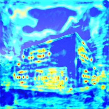
References                                                                  Berg. Ssd: Single shot multibox detector. In European con-
                                                                            ference on computer vision, pages 21–37. Springer, 2016. 3
 [1] Tensorflow lite. https://www.tensorflow.org/lite. 6
                                                                     [16]   Ilya Loshchilov and Frank Hutter.           Sgdr: Stochas-
 [2] Martı́n Abadi, Ashish Agarwal, Paul Barham, Eugene                     tic gradient descent with warm restarts. arXiv preprint
     Brevdo, Zhifeng Chen, Craig Citro, Greg S Corrado, Andy                arXiv:1608.03983, 2016. 6
     Davis, Jeffrey Dean, Matthieu Devin, et al. Tensorflow:
                                                                     [17]   Quan Meng, Jiakai Zhang, Qiang Hu, Xuming He, and
     Large-scale machine learning on heterogeneous distributed
                                                                            Jingyi Yu. Lgnn: A context-aware line segment detector. In
     systems. arXiv preprint arXiv:1603.04467, 2016. 6
                                                                            Proceedings of the 28th ACM International Conference on
 [3] Adrien Bartoli and Peter Sturm. Structure-from-motion
                                                                            Multimedia, pages 4364–4372, 2020. 2, 6, 7
     using lines: Representation, triangulation, and bundle ad-
     justment.     Computer vision and image understanding,          [18]   Branislav Micusik and Horst Wildenauer.             Structure
     100(3):416–441, 2005. 1                                                from motion with line segments under relaxed endpoint
                                                                            constraints. International Journal of Computer Vision,
 [4] Jia Deng, Wei Dong, Richard Socher, Li-Jia Li, Kai Li,
                                                                            124(1):65–79, 2017. 1
     and Li Fei-Fei. Imagenet: A large-scale hierarchical image
     database. In 2009 IEEE conference on computer vision and        [19]   Bronislav Přibyl, Pavel Zemčı́k, and Martin Čadı́k. Cam-
     pattern recognition, pages 248–255. Ieee, 2009. 6                      era pose estimation from lines using pl\” ucker coordinates.
                                                                            arXiv preprint arXiv:1608.02824, 2016. 1
 [5] Patrick Denis, James H Elder, and Francisco J Estrada. Ef-
     ficient edge-based methods for estimating manhattan frames      [20]   Bronislav Přibyl, Pavel Zemčı́k, and Martin Čadı́k. Abso-
     in urban imagery. In European conference on computer vi-               lute pose estimation from line correspondences using direct
     sion, pages 197–210. Springer, 2008. 1, 6                              linear transformation. Computer Vision and Image Under-
                                                                            standing, 161:130–144, 2017. 1
 [6] Olivier D Faugeras, Rachid Deriche, Hervé Mathieu,
     Nicholas Ayache, and Gregory Randall. The depth and mo-         [21]   Joseph Redmon, Santosh Divvala, Ross Girshick, and Ali
     tion analysis machine. In Parallel Image Processing, pages             Farhadi. You only look once: Unified, real-time object de-
     143–175. World Scientific, 1992. 1                                     tection. In Proceedings of the IEEE conference on computer
 [7] Ross Girshick. Fast r-cnn. In Proceedings of the IEEE inter-           vision and pattern recognition, pages 779–788, 2016. 3
     national conference on computer vision, pages 1440–1448,        [22]   Joseph Redmon and Ali Farhadi. Yolo9000: better, faster,
     2015. 2                                                                stronger. In Proceedings of the IEEE conference on computer
 [8] Ross Girshick, Jeff Donahue, Trevor Darrell, and Jitendra              vision and pattern recognition, pages 7263–7271, 2017. 3
     Malik. Rich feature hierarchies for accurate object detection   [23]   Joseph Redmon and Ali Farhadi. Yolov3: An incremental
     and semantic segmentation. In Proceedings of the IEEE con-             improvement. arXiv preprint arXiv:1804.02767, 2018. 3
     ference on computer vision and pattern recognition, pages       [24]   Shaoqing Ren, Kaiming He, Ross Girshick, and Jian Sun.
     580–587, 2014. 2                                                       Faster r-cnn: Towards real-time object detection with region
 [9] Andrew G Howard, Menglong Zhu, Bo Chen, Dmitry                         proposal networks. arXiv preprint arXiv:1506.01497, 2015.
     Kalenichenko, Weijun Wang, Tobias Weyand, Marco An-                    2
     dreetto, and Hartwig Adam. Mobilenets: Efficient convolu-       [25]   Mark Sandler, Andrew Howard, Menglong Zhu, Andrey Zh-
     tional neural networks for mobile vision applications. arXiv           moginov, and Liang-Chieh Chen. Mobilenetv2: Inverted
     preprint arXiv:1704.04861, 2017. 3                                     residuals and linear bottlenecks. In Proceedings of the
[10] Kun Huang and Shenghua Gao. Wireframe parsing with                     IEEE conference on computer vision and pattern recogni-
     guidance of distance map. IEEE Access, 7:141036–141044,                tion, pages 4510–4520, 2018. 3, 6
     2019. 1                                                         [26]   Ramprasaath R Selvaraju, Michael Cogswell, Abhishek Das,
[11] Kun Huang, Yifan Wang, Zihan Zhou, Tianjiao Ding,                      Ramakrishna Vedantam, Devi Parikh, and Dhruv Batra.
     Shenghua Gao, and Yi Ma. Learning to parse wireframes                  Grad-cam: Visual explanations from deep networks via
     in images of man-made environments. In Proceedings of the              gradient-based localization. In Proceedings of the IEEE in-
     IEEE Conference on Computer Vision and Pattern Recogni-                ternational conference on computer vision, pages 618–626,
     tion, pages 626–635, 2018. 1, 2, 6, 7, 8                               2017. 6
[12] Siyu Huang, Fangbo Qin, Pengfei Xiong, Ning Ding, Yijia         [27]   Rafael Grompone Von Gioi, Jeremie Jakubowicz, Jean-
     He, and Xiao Liu. Tp-lsd: Tri-points based line segment                Michel Morel, and Gregory Randall. Lsd: A fast line
     detector. arXiv preprint arXiv:2009.05505, 2020. 1, 2, 4, 6,           segment detector with a false detection control. IEEE
     7                                                                      transactions on pattern analysis and machine intelligence,
[13] Diederik P Kingma and Jimmy Ba. Adam: A method for                     32(4):722–732, 2008. 7
     stochastic optimization. arXiv preprint arXiv:1412.6980,        [28]   Robert J Wang, Xiang Li, and Charles X Ling. Pelee: A
     2014. 6                                                                real-time object detection system on mobile devices. arXiv
[14] Yuxi Li, Jiuwei Li, Weiyao Lin, and Jianguo Li. Tiny-dsod:             preprint arXiv:1804.06882, 2018. 3
     Lightweight object detection for resource-restricted usages.    [29]   Chi Xu, Lilian Zhang, Li Cheng, and Reinhard Koch. Pose
     arXiv preprint arXiv:1807.11013, 2018. 3                               estimation from line correspondences: A complete analysis
[15] Wei Liu, Dragomir Anguelov, Dumitru Erhan, Christian                   and a series of solutions. IEEE transactions on pattern anal-
     Szegedy, Scott Reed, Cheng-Yang Fu, and Alexander C                    ysis and machine intelligence, 39(6):1209–1222, 2016. 1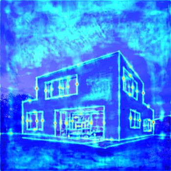
[30] Nan Xue, Song Bai, Fudong Wang, Gui-Song Xia, Tianfu
     Wu, and Liangpei Zhang. Learning attraction field represen-
     tation for robust line segment detection. In Proceedings of
     the IEEE/CVF Conference on Computer Vision and Pattern
     Recognition, pages 1595–1603, 2019. 1, 2, 6, 7
[31] Nan Xue, Tianfu Wu, Song Bai, Fudong Wang, Gui-Song
     Xia, Liangpei Zhang, and Philip HS Torr. Holistically-
     attracted wireframe parsing.       In Proceedings of the
     IEEE/CVF Conference on Computer Vision and Pattern
     Recognition, pages 2788–2797, 2020. 1, 2, 7
[32] Nan Xue, Gui-Song Xia, Xiang Bai, Liangpei Zhang, and
     Weiming Shen. Anisotropic-scale junction detection and
     matching for indoor images. IEEE Transactions on Image
     Processing, 27(1):78–91, 2017. 1
[33] Yuan Xue, Zihan Zhou, and Xiaolei Huang. Neural wire-
     frame renderer: Learning wireframe to image translations.
     arXiv preprint arXiv:1912.03840, 2019. 1
[34] Zhucun Xue, Nan Xue, Gui-Song Xia, and Weiming Shen.
     Learning to calibrate straight lines for fisheye image rec-
     tification. In Proceedings of the IEEE/CVF Conference
     on Computer Vision and Pattern Recognition, pages 1643–
     1651, 2019. 1
[35] Ziheng Zhang, Zhengxin Li, Ning Bi, Jia Zheng, Jinlei
     Wang, Kun Huang, Weixin Luo, Yanyu Xu, and Shenghua
     Gao. Ppgnet: Learning point-pair graph for line segment
     detection. In Proceedings of the IEEE/CVF Conference
     on Computer Vision and Pattern Recognition, pages 7105–
     7114, 2019. 1, 2, 6
[36] Yichao Zhou, Haozhi Qi, and Yi Ma. End-to-end wireframe
     parsing. In Proceedings of the IEEE/CVF International Con-
     ference on Computer Vision, pages 962–971, 2019. 1, 2, 6,
     7
Towards Light-weight and Real-time Line Segment Detection
Supplementary Material
A. Details of M-LSD Block Input SC input Operator c n
1 H×W×3 - conv2d 32 1
Architecture. The detailed architecture of M-LSD-tiny 2 H/2×W/2×32 - bottleneck 16 1
and M-LSD is described in Table A. M-LSD-tiny includes 3∼4 H/2×W/2×16 - bottleneck 24 2
an encoder structure from MobileNetV2 [4] in block 1∼11 5∼7 H/4×W/4×24 - bottleneck 32 3
and a custom decoder structure in block 12∼final. M- 8∼11 H/8×W/8×32 - bottleneck 64 4
LSD also includes an encoder structure from MobileNetV2 12 H/16×W/16×64 H/8×W/8×32 block type A 128 1
in block 1∼14 and a designed decoder structure in block 13 H/8×W/8×128 - block type B 64 1
14 H/8×W/8×64 H/4×W/4×24 block type A 64 1
15∼final, which is illustrated in Figure A. For the upscale 15 H/4×W/4×64 - block type B 64 1
operation, we use bilinear interpolation. 16 H/4×W/4×64 - block type C 16 1
- H/4×W/4×16 - upscale 16 1
Final H/2×W/2×16 - - - -
Feature Maps and Losses. For the displacement maps,
we compute displacement vectors from the ground truth (a) M-LSD-tiny
(GT) and mark those values on the center of line segment Block Input SC input Operator c n
in the GT map. Next, these values are extrapolated to a 1 H×W×3 - conv2d 32 1
3×3 window (center blob) so that all neighboring pixels of 2 H/2×W/2×32 - bottleneck 16 1
a given pixel contain the same value. For the displacement, 3∼4 H/2×W/2×16 - bottleneck 24 2
5∼7 H/4×W/4×24 - bottleneck 32 3
length, and degree maps, we use the smooth L1 loss for re- 8∼11 H/8×W/8×32 - bottleneck 64 4
gression learning. The regression loss can be formulated as 12∼14 H/16×W/16×64 - bottleneck 96 3
follows: 15 H/16×W/16×96 H/16×W/16×64 block type A 128 1
1 X 16 H/16×W/16×128 - block type B 64 1
`reg (F ) = P H(p) · Lsmooth
1 (F (p), F̂ (p)), (i) 17 H/16×W/16×64 H/8×W/8×32 block type A 128 1
p H(p) p 18 H/8×W/8×128 - block type B 64 1
19 H/8×W/8×64 H/4×W/4×24 block type A 128 1
where F (p) and F̂ (p) denote values of pixel p in the feature 20 H/4×W/4×128 - block type B 64 1
21 H/4×W/4×64 H/2×W/2×16 block type A 128 1
map F and the GT map F̂ , and H(p) outputs 1 if the pixel 22 H/2×W/2×128 - block type B 64 1
p of the GT map is on the center blob (extrapolated 3×3 23 H/2×W/2×64 - block type C 16 1
window). We use the displacement loss Ldisp = `reg (D), Final H/2×W/2×16 - - - -
where D denotes the displacement map. The length and
(b) M-LSD
degree losses are Llength = `reg (σ(L)) and Ldegree =
`reg (σ(G)), where σ(L) and σ(G) are sigmoid function σ Table A. Architecture details of M-LSD-tiny and M-LSD.
applied to length and degree maps. In the line generation Each line describes a sequence of 1 or repeating n identical
process, the center map is applied with a sigmoid function layers where each layer in the same sequence has the same
to output a probability value, while the displacement map c output channels. Block numbers (‘Block’) and block type
uses the original values. Then, we extract the exact center A∼C in ‘Operator’ are from Figure 3 and Figure A. ‘SC
point position by non-maximum suppression [1, 6, 2] on the input’ denotes a skip connection input and the bottleneck
center map to remove duplicates around correct predictions. operation is from MobileNetV2 [4].
Final Feature Maps. In the training phase, M-LSD-tiny
and M-LSD output final feature maps of 16 channels, which
include 7 channels for TP maps, 7 channels for SoL maps, inference phase. Thus, we disregard these operations and
and 2 channels for segmentation maps as illustrated in Fig- output only 5 channels of TP maps in the inference phase,
ure Ba. However, as the line generation process only re- including 1 center map and 4 displacement maps, as shown
quires the center and displacement maps of TP maps, op- in Figure Bb. As a result, we can minimize computational
erations for the other auxiliary maps are unnecessary in the cost and maximize the inference speed.Figure A. The overall architecture of M-LSD. In the feature extractor, block 1 ∼ 14 are parts of MobileNetV2, and block 15
∼ 23 are designed as a top-down architecture. The final feature maps are simply generated with upscale. The predicted line
segments are generated by merging center points and displacement vectors from the TP maps.
Table Ba, we vary the parts used from the MobileNetV2
on the encoder architecture. As the encoder size increases,
we add block types A and B to the decoder structure by
following the structural format in Table Ab. Model 1 ∼ 3
exploit bigger and deeper encoder architectures, which re-
sult in larger model parameters and slower inference speed.
The performance turns out to be slightly higher than that of
M-LSD. However, we choose ‘Input ∼ 96-channel’ of Mo-
(a) Final feature maps in the training phase bileNetV2 as the encoder for M-LSD because increasing the
encoder size causes larger amounts of model parameters to
be used and decreases the inference speed with a negligi-
ble performance boost. Moreover, we observe that ‘Input ∼
96-channel’ is the largest model that can work on a mobile
device in real-time. In contrast, when performing real-time
LSD on GPUs, model 1 ∼ 3 are good candidates as they
(b) Final feature maps in the inference phase outperform TP-LSD-Lite [2], previously the best real-time
LSD, with faster inference speed and lighter model size.
Figure B. Final feature maps in the training and inference
phase. (a) In the training phase, the final feature maps in- In Table Bb, we vary the block types used in the de-
clude TP, SoL, and segmentation maps with a total of 16 coder architecture. Model 4 changes every 1 × 1 convo-
channels. (b) For better efficiency in the inference phase, lution to a 3 × 3 convolution in block type A, while model 5
we disregard unnecessary convolutions and maintain only changes the residual connection from being in between the
the center and displacement maps in the TP maps with a convolutions (‘pre-residual’) to the end of the convolutions
total of 5 channels. (‘post-residual’) for block type B. These changes result in
an increase in model size and a decrease in inference speed
because ‘post-residual’ requires twice the number of output
B. Extended Experiments channels than that of ‘pre-residual’. However, the perfor-
mance remains similar to that of M-LSD-tiny. For models
B.1. Ablation Study of Architecture
6 and 7, the dilated rate of the first convolution in block
We run a series of ablation experiments to investigate type C is changed to 1 and 3, respectively. Here we observe
various encoder and decoder architectures. As shown in that by decreasing the dilated rate can improve the inferenceParams (M) Inference speed (FPS) Performance
Model Parts of MNV2 in encoder
Encoder (% of MNV2) Decoder Total Backbone Prediction Total FH sAP 10 LAP
M-LSD-tiny Input ∼ 64-channel 0.3 (7.4) 0.3 0.6 201.6 881.9 164.1 77.2 58.0 57.9
M-LSD Input ∼ 96-channel 0.6 (16.5) 0.9 1.5 132.8 883.4 115.4 80.0 62.1 61.5
1 Input ∼ 160-channel 1.0 (30.6) 1.3 2.3 124.7 885.1 109.3 79.9 62.8 62.4
2 Input ∼ 320-channel 1.8 (54.1) 1.5 3.3 117.9 885.7 104.0 79.7 62.5 62.6
3 Input ∼ 1280-channel 2.3 (66.5) 1.7 4.0 107.6 883.4 95.9 80.2 62.8 62.1
(a) Ablation study by varying the parts used from the MobileNetV2 (MNV2) for the encoder architecture. Performance is reported on
Wireframe dataset. ‘% of MNV2’ indicates the percentage of parameters used in each type of encoder compared to the total parameters
used in MobileNetV2.
Inference speed (FPS) Performance
Model Setup Params (M)
Backbone Prediction Total FH sAP 10 LAP
M-LSD-tiny Block type A: 1 × 1 conv / B: pre-residual / C: dilated rate 5 0.6 201.6 881.9 164.1 77.2 58.0 57.9
4 Block type A: 1 × 1 conv → 3 × 3 conv 0.7 199.2 881.9 162.5 76.7 58.1 57.9
5 Block type B: pre-residual → post-residual 0.7 200.5 881.9 163.4 76.9 58.1 58.0
6 Block type C: dilated rate 5 → 1 0.6 215.2 881.9 173.0 75.9 56.1 56.0
7 Block type C: dilated rate 5 → 3 0.6 203.5 881.9 165.3 76.7 57.6 57.4
(b) Ablation study by varying block types for the decoder architecture. Performance is reported on Wireframe dataset with M-LSD-tiny as
the baseline. Block type A ∼ B are from Figure 3 and Figure A.
Table B. Ablation study on encoder and decoder architectures.
speed but conversely decrease the performance. This is be- Setup Params
Inference speed (FPS) Performance
Backbone Prediction Total FH sAP 10 LAP
cause the dilated convolution can effectively manage long
w/o offset 629253 201.6 881.9 164.1 77.2 58.0 57.9
line segments, which require large receptive fields. Thus, w/ offset 629383 201.6 811.4 161.5 77.2 57.9 57.9
we choose to use 1 × 1 convolution in block type A, ‘pre-
residual’ in block type B, and the dilated rate of 5 in block Table C. Experiments of w/o and w/ offset maps in M-LSD-
type C. tiny on Wireframe dataset.
B.2. Needs of Offset Maps
In some of the previous LSD methods [3, 6, 5], offset of subparts µ is determined by µ = input size × . We con-
maps are used to estimate offsets between the predicted map duct an experiment to investigate the impact of ratio in
and input image because the predicted map has a smaller Table D. Small ratio will split line segments with a shorter
resolution than the input image. We perform experiments length while producing a greater number of subparts, and
and evaluate the effectiveness of offset maps with M-LSD- vice versa when using a large ratio . As shown in Ta-
tiny. When we apply offset maps to M-LSD-tiny, we need ble D, although a small ratio produces a large number
two offset maps for the center point (one for each coordi- of augmented line segments, performance improvement is
nate). As shown in Table C, w/ offset maps increase in small. This is because the center and end points of small
model parameters and decrease in inference speed, while subparts are too close to each other to be distinguished, and
the performance does not change. This demonstrates that thus become distractions for the model. Using a large ratio
offset maps are unnecessary for M-LSD-tiny because the also shows small performance improvement because not
resolution of the input image is two times the size of the only does the amount of augmented line segments decrease,
resolution of predicted maps, which is minor. Thus, we dis- but also these line segments result to resemble the original
regard offset maps in M-LSD architectures. line segment. We observe the proper ratio is 0.125, which
produces enough number of augmented line segments with
B.3. Impact of SoL Augmentation different lengths and location from the originals.
In SoL augmentation, the number of internally dividing When applying SoL augmentation, we split line seg-
points k is based on the length of the line segment and com- ments into multiple subparts with overlapping portions with
puted as k = br(l)/(µ/2)e − 1, where r(l) denotes the each other. To see the impact of retaining such overlap in
length of line segment l, and µ is the base length of the SoL augmentation, we conduct an experiment as shown in
subparts. Note that when k ≤ 1, we do not split the line Table E. W/o overlap shows a smaller performance boost
segment. When dividing the line segment, the base length than that of w/ overlap. Hence we conclude that using a µ # origin # aug # total FH sAP 10 LAP where the predicted line would be easily matched with the
0.000 - 374884 0 374884 76.2 55.1 55.3 GT line even if it is not similar. We conduct an experiment
0.050 25.6 374884 851555 1226439 76.2 56.2 56.3 to see the impact of the threshold γ in matching loss. As
0.100 51.2 374884 251952 626836 76.4 57.2 57.3
shown in Table F, when the threshold is high (γ ≥ 10.0), the
0.125 64.0 374884 151804 526688 77.2 58.0 57.9
0.150 76.8 374884 102719 477603 77.0 57.5 57.9 matching condition is too broad, and poses a higher chance
0.200 102.4 374884 47500 422384 76.6 56.8 56.5 of predicted lines matching with non-similar GT lines. This
0.300 153.6 374884 12123 387007 76.6 56.1 56.7 becomes a distraction and shows performance degradation.
0.400 204.8 374884 3250 378134 76.4 55.5 56.1
0.500 256.0 374884 170 375054 76.2 55.0 55.7
On the other hand, when the threshold is too low (γ = 2.5),
the matching condition is strict and consequently restrains
Table D. Impact of ratio in SoL augmentation with M- the effect of the matching loss to be minor due to the small
LSD-tiny on Wireframe dataset. = 0.0 is the baseline with number of matched lines. We observe that a value around
no SoL augmentation applied. The base length of subpart 5.0 is the proper threshold γ, which provides optimal bal-
µ is computed by µ = input size × . ‘# origin’, ‘# aug’, ance.
and ‘# total’ denote the number of original, augmented, and B.5. Precision and Recall Curve
total line segments.
We include Precision-Recall (PR) curves of sAP 10 for
# origin # aug # total FH sAP 10 LAP
L-CNN [6], HAWP [5], TP-LSD [2], and M-LSD (ours).
Figure C shows comparisons of PR curves on Wireframe
baseline 374884 - 374884 76.2 55.1 55.3
w/ overlap 374884 151804 526688 77.2 58.0 57.9 and YorkUrban datasets.
w/o overlap 374884 41101 415985 76.4 56.7 56.7
References
Table E. Impact of overlapping in SoL augmentation with [1] Kun Huang, Yifan Wang, Zihan Zhou, Tianjiao Ding,
M-LSD-tiny on Wireframe dataset. The baseline is not Shenghua Gao, and Yi Ma. Learning to parse wireframes
trained with SoL augmentation. ‘# origin’, ‘# aug’, and ‘# in images of man-made environments. In Proceedings of the
total’ denote the number of original, augmented, and total IEEE Conference on Computer Vision and Pattern Recogni-
line segments. tion, pages 626–635, 2018. i
[2] Siyu Huang, Fangbo Qin, Pengfei Xiong, Ning Ding, Yijia
Input size 320 Input size 512 He, and Xiao Liu. Tp-lsd: Tri-points based line segment de-
γ tector. arXiv preprint arXiv:2009.05505, 2020. i, ii, iv
FH sAP 10 LAP FH sAP 10 LAP
[3] Quan Meng, Jiakai Zhang, Qiang Hu, Xuming He, and Jingyi
0.0 75.9 47.1 44.9 76.1 55.1 54.8 Yu. Lgnn: A context-aware line segment detector. In Pro-
2.5 76.2 50.4 48.9 76.5 57.2 57.2 ceedings of the 28th ACM International Conference on Multi-
5.0 76.8 51.3 50.1 77.2 58.0 57.9 media, pages 4364–4372, 2020. iii
7.5 76.0 49.0 48.5 76.8 58.5 57.2 [4] Mark Sandler, Andrew Howard, Menglong Zhu, Andrey Zh-
10.0 75.0 45.1 45.0 76.8 57.8 56.7 moginov, and Liang-Chieh Chen. Mobilenetv2: Inverted
12.5 74.1 43.1 43.2 76.2 56.7 55.8 residuals and linear bottlenecks. In Proceedings of the IEEE
15.0 74.2 42.7 42.8 75.7 54.0 53.2 conference on computer vision and pattern recognition, pages
20.0 73.6 41.4 42.1 75.1 51.0 50.6 4510–4520, 2018. i
[5] Nan Xue, Tianfu Wu, Song Bai, Fudong Wang, Gui-Song Xia,
Table F. Impact of matching loss threshold γ with M-LSD- Liangpei Zhang, and Philip HS Torr. Holistically-attracted
tiny on Wireframe dataset. γ = 0.0 is the baseline with no wireframe parsing. In Proceedings of the IEEE/CVF Con-
matching loss applied. ference on Computer Vision and Pattern Recognition, pages
2788–2797, 2020. iii, iv
[6] Yichao Zhou, Haozhi Qi, and Yi Ma. End-to-end wireframe
larger number of augmented lines and preserving connec- parsing. In Proceedings of the IEEE/CVF International Con-
tivity among subparts with overlaps can yield higher per- ference on Computer Vision, pages 962–971, 2019. i, iii, iv
formance than without overlaps.
B.4. Threshold of Matching Loss
In the matching loss, the threshold γ decides whether to
match the predicted and GT line segments. When γ is small,
the matching condition becomes strict, where the predicted
line would be matched only with a highly similar GT line.
When γ is large, the matching condition becomes lenient,You can also read