Combinatorial approach to spreading processes on networks
←
→
Page content transcription
If your browser does not render page correctly, please read the page content below
Combinatorial approach to spreading processes on networks
                                                                                                   Dario Mazzilli1 and Filippo Radicchi1, ∗
                                                                                              1
                                                                                                Center for Complex Networks and Systems Research,
                                                                                            Luddy School of Informatics, Computing, and Engineering,
                                                                                              Indiana University, Bloomington, Indiana 47408, USA
                                                                      Stochastic spreading models defined on complex network topologies are used to mimic the diffusion of dis-
                                                                   eases, information, and opinions in real-world systems. Existing theoretical approaches to the characterization
                                                                   of the models in terms of microscopic configurations rely on some approximation of independence among dy-
                                                                   namical variables, thus introducing a systematic bias in the prediction of the ground-truth dynamics. Here,
                                                                   we develop a combinatorial framework based on the approximation that spreading may occur only along the
                                                                   shortest paths connecting pairs of nodes. The approximation overestimates dynamical correlations among node
                                                                   states and leads to biased predictions. Systematic bias is, however, pointing in the opposite direction of exist-
                                                                   ing approximations. We show that the combination of the two biased approaches generates predictions of the
                                                                   ground-truth dynamics that are more accurate than the ones given by the two approximations if used in isolation.
                                                                   We further take advantage of the combinatorial approximation to characterize theoretical properties of some in-
                                                                   ference problems, and show that the reconstruction of microscopic configurations is very sensitive to both the
arXiv:2101.02176v1 [physics.soc-ph] 6 Jan 2021

                                                                   place where and the time when partial knowledge of the system is acquired.

                                                                            I.   INTRODUCTION                                 of neglecting, to some extent, dynamical correlations that are
                                                                                                                              essential for the exact description of unidirectional spreading
                                                    Stochastic spreading models running on top of network                     processes. As a consequence, their predictions are systemati-
                                                 topologies have been used to study a large variety of real-                  cally biased towards the overestimation of the infection prob-
                                                 world dynamical processes [1–4]. Examples include the                        ability of individual nodes. From the computational point of
                                                 spread of diseases [5, 6], the diffusion of information and                  view, these approximations allow for the quick computation of
                                                 opinions [7–10], the propagation of bank failures [11],                      marginal probabilities. However, they lack of flexibility with
                                                 blackout cascades [12], development of countries [13], and                   respect to changes in the dynamical and/or topological details
                                                 avalanche dynamics in neural networks [14].                                  of the process. If the initial conditions of the dynamics, the pa-
                                                    In spite of their simplicity, many spreading models can be                rameter values of the spreading model, or the topology of the
                                                 solved exactly on very specific network topologies only; ex-                 network are changed, solutions of the approximations should
                                                 tensive simulations and/or theoretical approximations are gen-               be computed afresh by iteration.
                                                 erally required to characterize their properties on arbitrary net-              In this paper, we introduce an approximation based on a
                                                 works [1]. A complete solution of a spreading model on a                     combinatorial calculation of the spreading probability along
                                                 network consists in associating a probability to every possi-                the shortest path between pairs of nodes. The approximation
                                                 ble microscopic configuration of the system at each instant                  neglects that an infection may propagate along paths longer
                                                 of time. Such a detailed knowledge may not be required in                    than the shortest one. We derive close-form expressions of the
                                                 applications where the interest is centered around the macro-                approximation for the Susceptible-Infected and Susceptible-
                                                 scopic behavior of the system, e.g., outbreak size and/or du-                Infected-Recovered models started from a single source of in-
                                                 ration [15–18]. It is however required in many other ap-                     fection. On trees, our approach is exact, providing a geometric
                                                 plications of central importance for spreading processes on                  interpretation of correlations and joint probabilities between
                                                 networks as for example the problems of inferring the pa-                    pairs of nodes. We leverage such an intuitive interpretation
                                                 tient zero identity [19, 20], optimal sampling [21], and in-                 of the approach to study properties of the patient-zero prob-
                                                 fluence maximization [22]. Existing theoretical approaches                   lem and to compare different strategies of acquiring informa-
                                                 to the microscopic description of spreading processes on net-                tion about network configurations from partial observations.
                                                 works rely on some approximation of independence among                       In networks with loops, the approach systematically underes-
                                                 the state variables of the individual nodes. For example, the                timates the probability of infection of individual nodes. The
                                                 individual-node mean-field approximation assumes complete                    bias goes in the opposite direction of existing approximations
                                                 dynamical independence among state variables of the individ-                 for spreading processes on networks. The simultaneous use of
                                                 ual nodes [1, 23, 24]. Message-passing approximations, such                  the two types of approximations allows us to define a region
                                                 as those considered in Refs. [25–28], improve over the mean-                 where the true value of probabilities lies. Their combination
                                                 field approximation by relying on conditional independence                   improves the accuracy of each individual approximation. We
                                                 among pairs of variables, providing exact predictions on tree-               stress that the computationally demanding component of our
                                                 structured networks and excellent predictive power on arbi-                  approximation consists in finding the shortest path between
                                                 trary networks. These approximations have the common bias                    pairs of nodes. Probabilities of node states are then deter-
                                                                                                                              mined solely on such a geometric knowledge. As a result,
                                                                                                                              exploring the parameters’ space of a spreading model is very
                                                                                                                              efficient. We are aware of existing approaches that approx-
                                                 ∗   filiradi@indiana.edu                                                     imate spreading as happening on the shortest paths among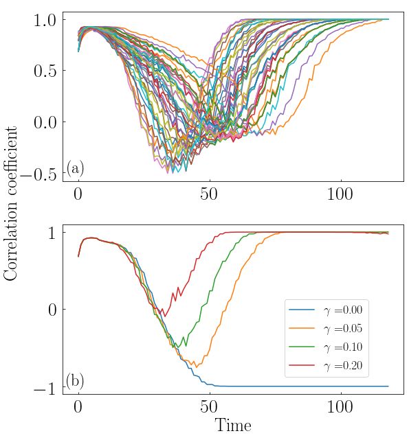
2

pairs of nodes only [29]. However, we are not aware of a            the same exact way as for the SI model. However, after all
full theoretical development of the approximation, consisting       spreading attempts of stage t have been considered, then ev-
of closed-form combinatorial solutions, as the one presented        ery node i such that σ(t−1)
                                                                                            i    = I may recover with probability
here.                                                               0 ≤ γ ≤ 1. Recovery of node i consists in the change of state
   The paper is organized as follows. In section II, we intro-      σ(t−1)
                                                                      i    = I → σ(t)i = R. After all recovery attempts have been
duce the spreading models considered in the paper. We fur-          considered, time increases as t → t + 1. Recovered nodes do
ther describe the individual-based mean-field approximation         not participate in the spreading dynamics, in the sense that
and our combinatorial approximation. We compare the accu-           they cannot infect their susceptible neighbors nor they can
racy of the approximations in predicting ground-truth spread-       be re-infected by their infected neighbors. Potentially many
ing dynamics. In the comparisons, we include also the dy-           different final configurations are reachable depending on the
namic message-passing approximation. In section III, we ap-         choice of the parameters β and γ, and the initial configuration
ply our approximation to trees, and characterize some proper-       of the system.
ties of inference problems associated to spreading, including
the identification of the patient zero and the maximization of
system information from the local observation of the states                         A.   The susceptible-infected model
of some nodes. In section IV, we summarize our results and
indicate viable extensions of our work.                                In this section, we derive analytical expressions for the SI
                                                                    model on arbitrary network topologies. We will first consider
                                                                    the individual-based mean-field approximation (IBMFA) [1,
       II. THEORETICAL APPROXIMATIONS FOR                           24, 32]. Then, we will derive a novel approximation based
         SPREADING DYNAMICS ON NETWORKS                             on combinatorial arguments. The novel approximation is ex-
                                                                    act on trees, and is expected to perform well on sparse tree-
   We assume that spreading occurs on a quenched, undirected        like networks. We name the method as the shortest-path com-
and unweighted, network composed of N nodes. The topol-             binatorial approximation (SPCA). We will characterize some
ogy of the network is fully specified by the N × N adjacency        properties of SPCA, and compare the prediction accuracy of
matrix A, whose generic element Ai j = A ji = 1 if nodes i and j    the novel approximation against IBMFA and the so-called dy-
are connected, whereas Ai j = A ji = 0, otherwise. We assume        namic message-passing approximation (DMPA) [26]. DMPA
that the network does not contain any self-connection, so that      is the best approximation on the market for the prediction of
Aii = 0 , ∀i. Without loss of generality, we further assume         marginal probabilities in the SI (and SIR) model. However,
that the network is composed of a single connected compo-           given their complicated form, we will not report DMPA equa-
nent, so that every node is reachable from any other node, and      tions below. The interested reader can find the equations, and
spreading from any single initial source node has the potential     their derivation, in Ref. [26].
to involve the entire system. We indicate with `i j the distance
between nodes i and j in the network, equal to the minimal
                                                                                                Problem setting
number of edges that separate the two nodes. Please note that
the symmetry of the network implies that `i j = ` ji .
   We consider the discrete-time version of two very popular           We assume that spreading is initiated by a single infected
models of spreading dynamics: the Susceptible-Infected (SI)         node s, i.e., σ(0)
                                                                                     s = I. Node s is the source of the infection or
and the Susceptible-Infected-Recovered (SIR) models [1, 30,         the patient zero. All other nodes j are initially in the suscepti-
31].                                                                ble state, i.e., σ(0)
                                                                                       ∀ j,s = S . Our goal is to fully characterize the
   In the SI model, every node i at time t can be found in two      probability of the microscopic state of every individual node
different states, either the susceptible state σ(t)
                                                i = S or the in-
                                                                    at each stage of the dynamics. The main quantity that we fo-
fected state σi(t) = I. At each discrete stage of the dynamics      cus on is
t > 0, every node i such that σ(t−1)    = I tries to infect every

                                   i                                  P(t)   = Prob.    σ (t−1)
                                                                                                = S → σ (t)
                                                                                                            = I  σ (0)
                                                                                                                         = S , σ(0)
                                                                                                                                    =  I    ,
neighbor j, i.e., Ai j = 1, in the susceptible state. The in-           s→i               i             i          ∀ j,s         s

fection is successfully transmitted with spreading probability                                                                             (1)
0 ≤ β ≤ 1. A successful spreading event consists in changing        i.e., the probability that the infection, started from the source
the state of node j as σ(t−1)   = S → σ(t)                          node s at time t = 0, reaches node i after exactly t stages of the
                                            j = I. This means
                            j
that the newly infected node j can attempt to further spread        dynamics. We will consider different expressions for P(t)         s→i on
the infection from time t + 1 on. After all spreading attempts      the basis of the above-mentioned approximations. Once P(t)             s→i
for all infected nodes have been considered, time increases as      is given, several other quantities useful in the characterization
t → t + 1. The dynamics is such that, as long as at least one       of the model dynamics can be immediately computed. For
node is initially infected and β > 0, all nodes will, sooner or     example, to obtain the probability Q(t)     s→i that node i has been
later, end up in the infected state.                                infected at time t or earlier, we simply perform the sum
   The SIR model is a slightly more sophisticated model than                                           t
the SI model, and the generic node i may be also found in
                                                                                                       X
                                                                                               s→i =
                                                                                              Q(t)             s→i .
                                                                                                              P(r)                        (2)
the recovered state σ(t) i   = R. Spreading events happen in                                            r=0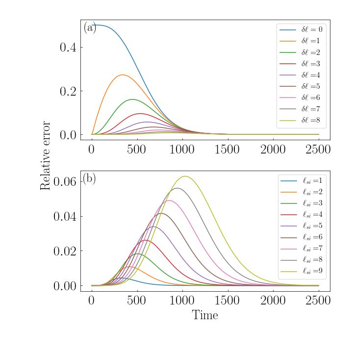
3
Based on our assumption on the initial configuration, we a given number of time steps, considering additional variables
automatically have that P(0)s→s = Q s→s = 1, and P s→i = Q s→i =
(0) (0) (0)
representing the states of pairs, triplets, etc. of nodes [6, 33].
0 , ∀ i , s. Better approximations require fully accounting for the unidi-
P(t) (t)
s→i and Q s→i are probabilities subjected to the initial con-
rectional motion of the infection along network edges. For
dition that spreading is initiated by node s. We can relax such example, Lokhov and collaborators [26] rely on conditional
a condition and consider arbitrary initial configurations con- independence among variables, and write equations of mes-
sisting of one unknown source. If we indicate with sages spreading along individual edges, in the same spirit as
h i done in approximations used in the study of percolation mod-
z s = Prob. σ(0)
∀ j,s = S , σ s = I
(0)
(3) els on networks [21, 34–37]. Their dynamic message-passing
approximation (DMPA) is exact on trees. In networks with
the probability that node s is the initial spreader, then the prob- loops, DMPA still leads to an overestimation of the true Q(t) s→i ,
ability P(t)
→i that node i receives the infection, from an arbitrary as the infection is allowed to travel in opposite directions on
initial spreader, at exactly stage t of the dynamics is estimated the same edge, although not immediately.
as
N
X
→i =
P(t) s→i .
z s P(t) (4) Shortest-path combinatorial approximation
s=1
The exact computation of P(t) s→i requires the enumeration of
Similarly, the probability Q(t)
→i that node i receives the infec- all possible ways in which the infection starting from node s
tion by an arbitrary single source at time t or earlier is given
reaches node i in exactly t time steps. Such an enumeration
by
includes all possible paths among the two nodes, and all pos-
N
X sible combinations for the propagation of the infection along
→i =
Q(t) s→i .
z s Q(t) (5) these paths. For an arbitrary network, the number of possi-
s=1 bilities grows exponentially with the system size, thus making
the exact computation of P(t) s→i infeasible. Here, we propose a
way to approximate from below P(t) s→i by simply assuming that
Individual-node mean-field approximation
the spread of the infection may happen only along the short-
est path connecting the nodes s and i, and then enumerating all
The individual-based mean-field approximation (IBMFA) possible ways in which the infection can propagate along such
consists in neglecting dynamical correlations among variables a path. We name the approximation as the shortest-path com-
so that every node i feels the average, over an infinite number binatorial approximation (SPCA). We stress that SPCA is ex-
of independent realizations of the spreading process, behavior act on trees, where each pair of nodes is connected by a unique
of its neighbors [1, 24, 32]. Under IBMFA, we can write path. We expect SPCA to provide a tight lower bound for the
h
i N
Y
ground-truth value of P(t) s→i in sparse loopy networks. Under
P s→i = 1 − Q s→i 1 −
(t) (t−1)
1 − A ji β Q s→ j .
(t−1)
(6) SPCA, P(t) s→i is uniquely determined by the distance ` si > 0
j=1 between nodes s and i. We can write
Eq. (6) is derived as follows. The probability for node i to
!
t − 1 `si
be infected at exactly time t is given by the product that the P(t) = β (1 − β)t−`si . (7)
s→i
` si − 1
node has been not infected at any time earlier than t, i.e.,
1 − Q(t−1)
s→i , and receives the infection by at least one
of its in-
Q Eq. (7) is derived as follows. We can think of the path s → i
fected neighbors, i.e., 1 − Nj=1 1 − A ji β Q(t−1)
s→ j . The latter as composed of two pieces, s → j and j → i, where j is the
term is computed as the product of individual contributions of nearest neighbor of node i along the path s → i, so that the dis-
the node’s neighbors, thus assuming complete independence tance between s and j is ` s j = ` si − 1, as in Figure 1. At stage t
of their states. of the dynamics, the final spreading attempt j → i must be, by
Eq. (6), together with Eq. (2), defines a system of N equa-
definition of P(t)
s→i , successful. This elementary event happens
tions, one for every node i. Solutions are obtained by iteration,
with probability β. However before the final step, the infection
starting from the imposed initial conditions.
must have reached node j and not moved further than node j
Limitations of IBMFA are apparent. Neglecting dynam-
in the preceding t − 1 steps of the dynamics. This fact happens
ical correlations leads to the possibility for the infection to
spread in opposite directions along the same edge, a situa- with probability equal to `t−1 si −1
β`si −1 (1−β)t−`si , corresponding
tion that is indeed impossible in SI dynamics. Because of to the binomial probability of observing exactly ` si −1 success-
this fact, the cumulative probability Q(t) ful spreading events in t − 1 total spreading attempts. Eq. (7)
s→i always overesti-
mates the true probability value, thus providing a consistent is finally given by the product of above-defined probabilities
upper bound for the ground truth. Approximations more pre- for the two pieces s → j and j → i of the path s → i.
cise than IBMFA can be obtained by accounting for dynami- Q(t)
s→i is obtained relying on Eq. (2). It is easy to check that
cal correlations tracing back the evolution of the system over limt→∞ Q(t) s→i = 1, for all nodes i and for any source node s, as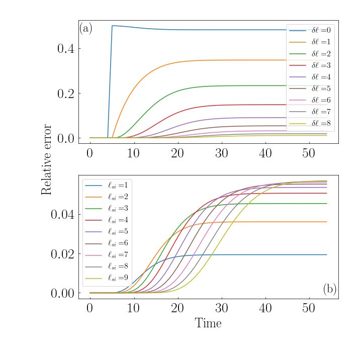
4

                                   4
                                                  5
                                   β
                   3                            (1-β)
                   β
                                            j
                                                                   i
       1                                                β
       β                                                6
                (1-β)
                   2
   S

Figure 1. The shortest-path combinatorial approximation. The figure
serves to illustrate the rationale behind Eq. (7). Here, we represent
a specific sequence of spreading attempts that allow the infection to
spread from the source node s to node i at distance ` si = 4 in exactly
t = 6 time dynamical steps. The sequence consists of four successful
                                                                          Figure 2. Error committed by the shortest-path combinatorial ap-
spreading events, and two unsuccessful spreading attempts, thus the
                                                                          proximation. Relative error of the SPCA compared to the ground-
probability of the sequence is β4 (1 − β)2 .
                                                                          truth value for the probability Q(t)
                                                                                                            s→i that node i is infected at time t or
                                                                          earlier by an infection starting from node s. Spreading obeys SI dy-
                                                                          namics with spreading probability β = 0.01. Ground-truth values are
expected for the SI model. Regardless of its distance from the            estimated under the hypothesis that nodes s and i are connected by
source, every node will be eventually infected.                           two independent paths of length ` si and ` si + d`, respectively. SPCA
    To get a sense of the magnitude of the approximation er-              approximates truth probabilities relying on the shortest path only. (a)
ror introduced by SPCA, we consider the case where nodes                  We set ` si = 5 and consider different values of d`. Relative error
s and i are connected by two independent paths of length                  is plotted as a function of time. (b) We set d` = 5, and consider
` si and ` si + d`, respectively. We focus our attention on the           different ` si values.
probability Q(t)s→i that the infection reaches node i at time t or
earlier. Such a probability is given by the likelihood that in-
fection propagates along at least one of the two independent              transportation network of Ref. [38]. The network has N = 500
paths, and its ground-truth value can be calculated exactly re-           nodes, density of connections ρ ' 0.024, and diameter d = 7.
lying on a proper combination of Eqs. (2) and (7), see ap-                Results are averages from random initial placements of the
pendix for details. We compare the ground-truth value with                source of the infection, thus, in the various theoretical approx-
the one we obtain using SPCA, and quantify the relative error             imations, the prior of Eq. (3) is taken equal to the uniform
of the approximation with respect to the truth value. Results             distribution, i.e., z s = 1/N.
for some combinations of the parameter values ` si and d` are                While taking into account only the shortest path is an over-
plotted in Figure 2. Relative error is a decreasing function              simplification of the problem, combining SPCA with IBMFA
of d`. It is worth noting that the relative error behaves non-            (or DMPA), as for example by taking the arithmetic average
monotonically as a function of time t, reaching a maximum at              of the two approximations, can increase the accuracy of the
intermediate t values.                                                    individual methods. This is especially true for sources of the
                                                                          process with low degree.

                 Predictions in real-world networks
                                                                                    B.   The susceptible-infected-recovered model

   A nice property of SPCA is to provide a consistent lower-
                                                                                                      Problem setting
bound for ground-truth probabilities. SPCA neglects that
spreading may occur along longer paths. The simultane-
ous use of IBMFA (or similar approaches that provide upper                   For SIR dynamics, we consider the same initial configura-
bounds for true probabilities, e.g., DMPA) and SPCA is very               tion as in the SI model, where spreading is initiated by a single
useful, as it allows us to delineate the region of possible out-          infected node s, i.e., σ(0)
                                                                                                   s = I, while all other nodes j are ini-
comes for the SI model. In Figure 3 for example, we compare               tially in the susceptible state, i.e., σ(0)
                                                                                                                  ∀ j,s = S . The probability
predictions of IBMFA, DMPA and SPCA with estimates of                     that node i receives the infection at exactly time t is defined in
the ground-truth probabilities obtained via numerical simula-             the same identical way as for the SI model, see Eq. (1). We
tions of the SI process on a real network. We use the US air              can further apply the same definition as in Eq. (2) to quan-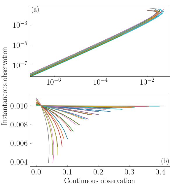
5
Eq. (9) is a direct generalization of Eq. (6). The mean-
ing of the various terms is exactly the same as in Eq. (6),
with the only difference that here we need to account for
the possibility of infected nodes to recover. To become in-
fected, we require that node i is still in the susceptible state
at time t, i.e., 1 − Q(t−1)
s→i , and that infection arrives from at
least one of
h its neighbors
that is still
i in the infected state, i.e.,
1 − j=1 1 − A ji β Q s→ j − T s→ j .
(t−1) (t−1)
QN
Properties and limitations of IBMFA for the SIR model are
very similar to those already illustrated for the SI model. Lim-
itations of Eq. (9) in capturing the true probability are due to
the assumption of dynamical independence among variables
that is in contrast with the unidirectional nature of spreading.
Still, IBMFA can be improved by imposing only conditional
independence instead of full independence among variables
as done in DMPA [26]. Also, IBMFA and DMPA continue to
provide effective methods to bound from the above marginal
probabilities of infection of the true SIR model.
Shortest-path combinatorial approximation
Figure 3. Accuracy of the approximations in predicting ground-truth
infection probabilities in real-world networks. We considered the SI
model on the air transportation network of Ref. [38]. The spread- In this section, we extend SPCA to the SIR model. The
ing probability is set β = 0.25. We run 4, 000 numerical simulations probability that node i is infected exactly at time t, given that
of the process where a given node is the source of the spreading. the infection started from the source node s, is
Ground-truth values are compared with predictions from the IBMFA !
t−` si t − 1
(green), SPCA (blue), DMPA (red), the average SPCA-IBMFA (pur- P(t) = (1 − γ) β`si (1 − β)t−`si . (10)
ple) and SPCA-DMPA (black). a) Mean absolute error over all pos- s→i
` si − 1
sible sources as a function of time. b) We display the absolute error
averaged over time as a function of the degree of the source node. Eq. (10) simply generalizes Eq. (7) with the inclusion of the
multiplicative factor (1 − γ)t−`si . This factor accounts for even-
tual recovery events that may prevent the infection to reach
tify the probability Q(t)
s→i that the infection reaches node i at
node i. As the infection can proceed its trajectory as long as
time t or earlier. The additional recovered state that is allowed the latest infected node does not recover before passing the
in the SIR model requires the definition of other probabilities infection, then the condition that allows spreading to occur is
not defined for the SI model. For instance, the probability that recovery should not happen in t−` si independent attempts,
that node i recovers exactly at time t, given that the infection leading to the factor (1 − γ)t−`si .
started from node s, is denoted by R(t) We can immediately derive that
s→i . The probability that
node i recovers at time t or earlier is given by !−`
(t) γ si
lim Q = 1−γ+ , (11)
t
X t→∞ s→i β
(t)
T s→i = s→i .
R(r) (8)
r=0 thus, in the long-term limit, the probability of infection ex-
ponentially decreases towards zero as the distance from the
All other probabilities of interest can be immediately derived. source increases.
For example, we have that the probability that node i is still in In spite of the fact that Eq. (11) is valid for individual nodes
the susceptible state at time t is given by 1 − Q(t)
s→i . Also, the only, we find that the equation is useful for the prediction of
probability that node i is found infected at time t is given by the outbreak of the entire system. In Figure 4, we compare the
Q(t) (t)
s→i − T s→i .
average value of the outbreak size estimated from numerical
simulations with predictions quantified as
!−h`i
Individual-based mean-field approximation γ
O= 1−γ+ , (12)
β
Under IBMFA [1, 24, 32], we can write
where h`i = N(N−1) 2
i> j `i, j is the average value of the dis-
P
h i
YN h (t−1) i
tance among nodes in the network. While predictions do not
P s→i = 1 − Q s→i
(t) (t−1)
1− 1 − A ji β Q s→ j − T s→ j
(t−1)
. match truth values, their functional similarity is apparent as
j=1
shown by the magnitude of the mismatch between ground-
(9) truth values and predictions.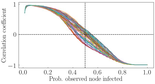
6

                                                                          Figure 5. Error committed by the shortest-path combinatorial ap-
                                                                          proximation. Same as in Figure 2 but for the SIR model. Spreading
                                                                          probability is β = 0.5, while recovery probability is γ = 0.5.
Figure 4. Prediction of the phase diagram under the shortest-path
combinatorial approximation. a) We consider a tree with N = 50
nodes and uniformly distributed random Prüfer sequence [39, 40].
We display the ground-truth value of the outbreak size, estimated
                                                                          presence of multiple paths connecting two nodes plays a much
from numerical simulations, as a function of the spreading and re-        more important role than in the SI model.
covery probabilities. The two black curves correspond to the solu-
tions of Eq. (12) obtained by setting respectively O = 0.5 (full curve)
and O = 0.01 (dashed). b) Difference between ground-truth values
of the outbreak size and predictions from Eq. (12) as a function of                      Predictions in real-world networks
the SIR model parameters.
                                                                             The considerations made for the SI model are still valid for
                                                                          the SIR model. In networks with loops, SPCA underestimates
  The probability to recover at time t is given by                        the ground-truth probability Q(t)
                                                                                                         s→i , while DMPA overestimates
                                    t−1
                                                                          it. The combination of SPCA and DMPA defines the region
                                                                          where the true values are located. Also, it is possible to im-
                                    X
              s→i = γ (1 − γ)
             R(t)             t−1
                                           s→i (1 − γ)
                                          P(r)         −r
                                                          .       (13)
                                    r=0
                                                                          prove the accuracy of the individual approximations by simply
                                                                          taking their arithmetic average, see Figure 6. Improvements
Eq. (13) is easily obtained considering that node i can recover           are especially apparent in the supercritical regime of the dy-
only if previously infected, say at time r. Then, the probabil-           namics, where the SIR model behaves most similarly to the SI
ity that recovery happens after a certain number of additional            model.
time steps is given by the probability that recovery happened
at time t but didn’t happen in any of the previous stages, i.e.,
γ (1 − γ)t−r−1 . Summing up over all possible time steps r when
node i could have been infected, one obtains Eq. (13).                                        III.   APPLICATIONS
   In Figure 5, we repeat the same exercise as in Figure 2 by
estimating the relative error committed by SPCA when the                     We now turn our attention to specific applications of the
ground-truth topology is such that nodes s and i are connected            theoretical framework in inference problems. We remark that
by two independent paths of length ` si and ` si + d`, respec-            we are not leveraging the framework to actually perform in-
tively. We note that the behaviour in the early stages of the             ference. Rather, we are using it to provide insights on the
relative error is quite similar to the SI case. Results for the           properties of the inference problems, as for example how the
SIR model differ from those of the SI model in the late stages            ability of an observer to perform inference is affected by the
of the dynamics, when the finite limit in Eq. (11) gives a non-           time of the observations and the position of the observer in the
vanishing asymptotic value. For the SIR model, the eventual               system.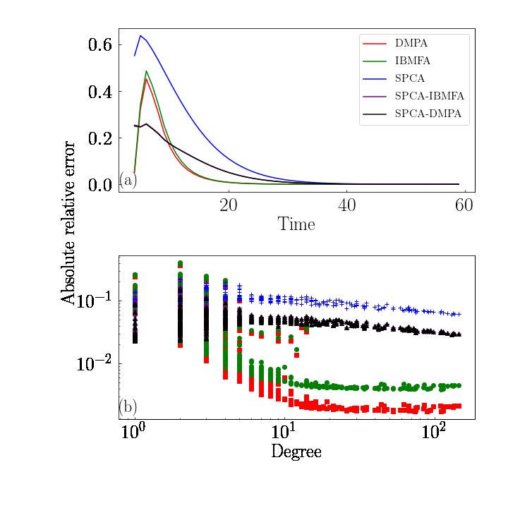
7

Figure 6. Accuracy of the approximations in predicting ground-truth infection probabilities in real-world networks. a) We consider the SIR
model on the air transportation network of Ref. [38]. We set β = 0.1 and γ = 0.1. The combination of the two parameter values correspond
to the supercritical regime of the dynamics. We run 8, 000 numerical simulations of the SIR process for each node being the source of the
infection to obtain a single estimate of the ground-truth values of Q(t)
                                                                     →i for all i. Ground-truth values are compared with predictions from the
IBMFA (green), SPCA (blue), DMPA (red), the average SPCA-IBMFA (purple) and the average SPCA-DMPA (black). The figure displays
the relative error, averaged over all nodes, committed by the various approximations as a function of time. b) Absolute error, averaged over
time, of the various approximations as a function of the degree of the source node. Data are the same as in panel a. c) Same as in panel a, but
for β = 0.01, corresponding to the subcritical regime of spreading. d) Same as in panel b, but obtained for the same parameter setting as in
panel c.

          A.   Identification of the source of spreading                  be written as

                                                                                                     (t)     z s P(t)
   As a first application, we consider the classical inference                                     V s→i =        s→i
                                                                                                                        ,                 (14)
problem aiming at the identification of the initial spreader, i.e.,                                           P(t)
                                                                                                               →i
the so-called patient-zero problem [41–43]. We note that the
problem has been already studied with a combinatorial ap-                 where P(t)          (t)
                                                                                    s→i and P→i are the same probabilities as defined in
proach similar to ours in Ref. [44]. The patient-zero problem             Eqs. (4) and (7), respectively. z s , defined in Eq. (3), is the
is typically framed under the assumption of limited informa-              probability that node s is the source of the infection prior any
tion, where only partial knowledge of the microscopic proper-             type of measurement made on the system.
ties of the system is available to the observer. In this paper, we           Second, we consider the case where the observer performs
focus on two different settings often considered in the litera-           a single measurement of node i at time t and finds it infected.
ture on this subject. In both cases, we assume that the observer          Infection may have occurred at time t or earlier. The proba-
has full and exact knowledge of the network topology. In ad-                       (t)
                                                                          bility W s→i that node s is the source of the infection under this
dition, the observer is fully aware of the stage of the dynamics          condition is given by
as well as of the exact values of the spreading and recovery
probabilities.                                                                                               z s Q(t)
                                                                                                    (t)
                                                                                                  W s→i =         s→i
                                                                                                                        .                 (15)
                                                                                                               Q(t)
                                                                                                                →i

                    Susceptible-infected model                            Here, z s is still our prior on the node s acting as the source
                                                                          of the infection; Q(t)          (t)
                                                                                                s→i and Q→i are the same probabilities as
   First, we consider the case where the observer is allowed              defined in Eqs. (2) and (5), respectively.
                                                                                                        (t)         (t)
to constantly monitor the state of node i. Suppose that, at                  A comparison between V s→i       and W s→i is illustrated in Fig-
time t, node i gets infected, and the observer wants to infer the         ure 7. The two strategies of performing local observations
                                                 (t)
identity of the patient zero. The probability V s→i  that node s          of the network generally lead to different predictions about
is the initial spreader is given by the Bayes’ theorem and can            the location of the patient zero, and the difference among the
8
(t)
two strategies strongly depends on the time when the mea- we display the Spearman correlation coefficient between V s→i
surements are performed. (t) (t)
and W s→i as a function of Q→i . Correlation is only mildly de-
pendent on the node where the system is observed from. The
non-perfect correlation found at very low values of Q(t) →i is still
surprising, but can be easily understood. If one finds the ob-
served node infected at the very first stages of the dynamics
without knowing exactly the time when the node was infected,
then it is very likely that the node itself is inferred to be the pa-
tient zero. However, when one knows that the exact time of in-
fection, one can properly distinguish cases when the observed
node was or was not the actual source of spreading. There
are two remarkable aspects emerging from Figure 8. First, the
change in sign of the correlation coefficient is happening at
Q(t)
→i ' 0.5. Second, the correlation coefficient becomes max-
imally negative well before Q(t) →i ' 1. This is due the fact
that, at very late stages of the spreading when all nodes are
likely to be found infected, having knowledge that the infec-
tion happened at a very late stage makes likely that the source
of infection was far apart from the observation point; not hav-
ing knowledge of the exact time of infection leads instead to
an almost flat probability distribution for the patient zero lo-
cation but still with a very weak preference for nodes close to
the observation point, including the observed node itself.
Figure 7. Comparison of observation strategies in the patient-zero
identification problem. We display the inferred probabilities on the
location of the source s obtained under the hypothesis of continuous
(t)
observation of the state of nodes, i.e., V s→i as defined in Eq. (14),
and under the hypothesis of instantaneous observation of their state,
(t)
i.e., W s→i as defined in Eq. (15). Each curve corresponds to a single
measured node i at time t; the curve is obtained by connecting pairs
(t)
of contiguous points (V s→i , W s→i
(t)
) for all s , i. The two panels show
results valid for two different values of the time of measurement,
namely t = 12 in panel a and t = 90 in panel b. Results are obtained
on a tree with N = 100 nodes and uniformly distributed random
Prüfer sequence [39, 40]. Spreading is happening according to the SI
model with spreading probability β = 0.3.
Figure 8. Comparison of observation strategies in the patient-zero
identification problem. Spearman correlation coefficient obtained by
In the early stages of the spreading process, the values of ranking nodes according to the inferred probabilities of being the
(t) (t)
V s→i or W s→i are highly heterogeneous, and the two strate- source of spreading according to instantaneous and continuous ob-
gies of observation lead to almost identical inferred proba- servation of the state of a node. The correlation coefficient is plotted
bilities regardless of the point of observation i. This fact is against the probability to find the observed node i infected. Different
easily explained as the most likely source of infection should curves correspond to different nodes observed, and different values
be located in the vicinity of the node where the system is ob- of the probability to find the observed node infected map to different
stages of the dynamics. Results are obtained in the same experimen-
served from. At later stages of the dynamics, the probability
(t) (t) tal setting as of Figure 7.
values V s→i or W s→i are less heterogeneous, the two inferred
probabilities are negatively correlated, and their discrepancy
strongly depends on the node i where the system is observed
from. The negative correlation in the final stages of the dy-
namics seems surprising but can be intuitively explained. If Susceptible-infected-recovered model
a node gets infected after a very long time, it is very unlikely
that the infection started from one of its neighbors. However, In the SIR model, three outcomes are possible when the
if one finds the node infected but does not know when the in- state of a node is measured. As a consequence, four differ-
fection happened, still the nearest nodes are the most likely ent conditional probabilities are potentially relevant for the
sources of infection. patient-zero identification problem. However, finding the ob-
The quantity that best characterizes the correlation between served node in the infected vs. recovered state does not gener-
(t) (t)
the inferred probabilities V s→i and W s→i is Q(t)
→i , i.e., the prob- ate a significant difference in our ability to predict the identify
ability to find node i infected at time t or earlier. In Figure 8, of the patient zero.9
In Figure 8, we measure the correlation between the in- B. Gain of information from local measurements
(t) (t)
ferred probabilities V s→i and W s→i on the location of the pa-
tient zero. We notice that the two strategies of observation What is the amount of information, about the microscopic
may lead to very different outcomes depending on either the configuration of the system, that we can gain by observing the
time when the observation is made and the values of the pa- state of a specific node? Clearly, as states of different nodes
rameters of the spreading model. Clearly, for γ = 0 we re- in the network are correlated, the measurement of the state of
cover the same results as of the SI model, with correlation one node provides us with some knowledge about the state of
never increasing as a function of time. For values of the recov- the other nodes. However, the gain of information will be not
ery probability γ > 0, correlation is instead a non-monotonic the same for all choices of the observed node; further, the gain
function of time. At early stages of the dynamics, correlation of information may dramatically vary, even if we decide to ob-
decreases for the same reasons as in the SI model. At late serve the same node, depending on the stage of the dynamics
stages, however, it increases. The reason is quite intuitive. when the measurement is performed.
Finding a node infected but not yet recovered at a late stage As a second application of our framework, we study spread-
of the dynamics means that it is unlikely that the node got in- ing processes from a information-theoretical perspective pro-
fected at the very beginning process, otherwise it would have viding indications about the content of information that each
had plenty of time to recover. Thus, knowing or not know- node carries about the whole network.
ing the exact time of infection is irrelevant for the patient-zero To properly quantify the gain of information we should cal-
inference problem, as one can exclude that the source of in- culate the mutual information between network configurations
fection is very close to the observed node in either cases. and the state of the observed node. This calculation would re-
quire to estimate the probability of every network configura-
tion conditioned by the state of the observed node, and then
a sum over all the possible conditional probabilities. Due to
the huge number of possible configurations however, the ex-
act computation of the information gain is infeasible. Here,
we approximate it as the sum of the pairwise mutual informa-
tion of all pairs of nodes. We compute the mutual information
among pairs of nodes i and j using their joint probability of
getting infected at time t or earlier, namely Q(t)
s→i, j . The geo-
metric framework of SPCA easily adapts to such a computa-
tion. Specifically, the computation of the joint probability still
relies on the definition of marginal probabilities, but properly
accounts for the possible paths between the source s and the
two target nodes i and j we are interested in (see Appendix
for details). The expected information gained by observing
node i is then quantified as the sum of the pairwise mutual
information of the node with respect to all other nodes in the
network.
Susceptible-infected model
Naively, we should expect that nodes that occupy central
positions in the network correspond to optimal points of ob-
servations. Such an intuition is generally correct, but with
some caveat. In Figure 10, we show the information gained
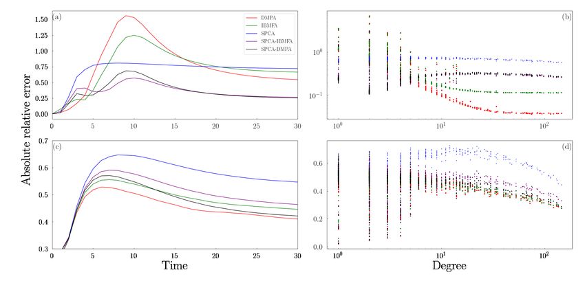
Figure 9. Comparison of observation strategies in the patient-zero by measuring a single node as a function of its degree, i.e., a
identification problem in the SIR model. a) Spearman correlation simple metric of network centrality. We considered metrics of
coefficient obtained by ranking nodes according to the inferred prob- network centrality more complicated than degree, but the re-
abilities of being the source of spreading according to instantaneous
sults of the analysis are qualitatively similar to those reported
and continuous observation of the state of a node. The correlation
coefficient is plotted against time. Different curves correspond to here. In the early stages of the dynamics, the information gain
different nodes observed. Results are obtained in the same config- is correlated with node degree. At late stages, observing the
uration as of Figure 7. Spreading probability is set β = 0.2, while network from nodes with large degrees becomes sub-optimal.
recovery probability is set γ = 0.1. b) Same as in panel a, but for The time of the measurement plays a fundamental role for
different γ values. Irrespective of the specific value of the recovery the amount of information that can be actually gained. At the
probability, the system is always observed from the same node. beginning of the dynamics, all nodes are in the susceptible
state, thus we do not expect any measurement to be informa-
tive. Similar conclusions are valid for the late stages of the
dynamics, when all nodes are likely to be in the infected state.10
We expect, however, measurements to be informative when
uncertainty about the system configuration is maximal. This
fact is apparent from Figure 10. We see that there is an inter-
mediate stage of the dynamics where the information content
of the network reaches a peak value. At that point in time, the
information gained by observing a node is not strongly de-
pendent on the centrality of the node where the observation is
performed.
Figure 11. Gain of information from local network measurements
in the SIR model. Total information content of the network as a
function of time for three different values of γ. We set β = 0.2 and
consider the same network as in Figure 9.
IV. CONCLUSIONS
In this paper, we presented a combinatorial approach to cal-
culate the spreading probability, along the shortest path be-
tween pairs of nodes in a network, for the Susceptible-Infected
(SI) and the Susceptible-Infected-Recovered (SIR) models.
We named it as the shortest-path combinatorial approxima-
tion (SPCA). The approach is exact in absence of loops and
gives a lower bound for the infection probability on arbitrary
networks. The approximation can be in principle extended to
include the effect of other paths (i.e., the second shortest path,
Figure 10. Gain of information from local network measurements in the third shortest path, etc.) on the computation of the spread-
the SI model. a) Gain of information obtained from the observation ing probability. However, adding more paths exponentially
of a single node. Information gain is plotted against the degree of increases the complexity of the algorithm, since the proce-
the observed node. Each point in the plot corresponds to a different dure requires to disentangle independent vs. shared parts (i.e.,
node used to observe the system. Different colors and symbols stand nodes and edges) among the various paths. We showed that
for different stages of the dynamical process when the observation the arithmetic average between the novel approximation and
is performed. The experimental setting is the same as in Figure 7. other approximations existing on the market, e.g., individual-
b) Total information content of the network as a function of time. node mean-field and dynamic message-passing approxima-
Information content P is measured(t) as the sum(t) of the individual-node tions, can be used to obtain predictions that are more accurate
entropies, i.e., I = i [Q(t)
→i log Q→i + (1 − Q→i ) log(1 − Q→i )].
(t)
than those obtained by each approximation if used in isolation.
The amount of improvement strongly depends on the degree
of the source and, in the SIR model, on the regime of the pro-
cess, hinting that the importance of the shortest path depends
on network’s connectivity as well as on the process’s param-
eters. Potential follow-up studies could explore the predictive
Susceptible-infected-recovered model power of more sophisticated ways than the arithmetic aver-
age to combine SPCA with other approximations. On a tree
network, we used SPCA to evaluate joint probabilities among
In Figure 11, we perform a similar analysis as of Figure 10, pairs of node states, and applied it to study general properties
but for the SIR model. The content of information as a func- of standard inference problems. Specifically, we character-
tion of time behaves in a different way depending on the ized two different strategies of single-node observation in the
choice of the parameters β and γ. If the probability of recov- identification problem of the patient zero. We showed that the
ery γ is low, then the information content of the SIR model is inference problem is highly sensitive to the modality in which
almost identical to the one we just described for the SI model. the observation is performed. Measuring a node at a given
If γ values are large enough instead, information content does time or monitoring it throughout the process may lead to op-
not longer decrease as time increases, reflecting the non-null posite conclusions on the identity of the patient zero. Also, we
uncertainty of the final configurations reached by SIR spread- analyzed the entropy of the processes and quantified the in-
ing. formation gained, when the state of a node is measured, about11
the rest of the network. The most informative node is not the Susceptible-infected-recovered model
same throughout the entire process and the knowledge of the
dynamical stage is crucial to optimize the information gained For the SIR model, the calculation is a bit more cumber-
by a measurement. These results can be extended by consider- some than for the SI model.
ing the measurements, contemporaneous or sequential, of two Suppose node s is initially in the infected state, and suppose
nodes. By calculating a three-node joint probability one could that two independent paths of length ` and ` +d` connect node
measure the most informative pair of nodes and study differ- i to node s. The probability q2 (`, ` + d`, t) that node i becomes
ent strategies for nodes’ control. While we focused only on infected at time t is given by the probability that the infection
the SI and SIR models, other spreading processes in discrete spreads along at least one of these paths. We remark that we
time can be studied with a similar theoretical approach. know the analytical form of the probability q1 (`, t) that the in-
fection spreads along a single path of length ` in t time steps
or less, see main text. However, this expression can be used
ACKNOWLEDGMENTS
to combine the contribution of the two independent paths only
provided that the paths are dynamically independent. The lat-
DM and FR acknowledge support from the US Army Re- ter condition is satisfied only when the infection performs at
search Office (W911NF-16-1- 0104). FR acknowledges sup- least one step towards the target along at least one of the paths.
port from the National Science Foundation (CMMI-1552487). Indicate with v the neighbor of node s along the path of
length ` towards i, and with w the neighbor of node s along
the path of length ` + d` towards i. The initial configura-
Appendix A: Magnitude of the error associated with the
tion at time t = 0 is such that σ(0) s = I and σ(0)
∀ j,s = S .
shortest-path combinatorial approximation
At time t = 1, the states of nodes may change as the re-
sults of spreading and recovery events. The only nodes that
In Figures 2 and 5, we considered an hypothetical setting can change their states are s, v and w. For example, we
where the generic node i is connected to the source node s by can go to the configuration σ(1) = (I, I, S , . . .), i.e., such that
two independent paths of length ` si and ` si + d`, with d` ≥
σ(1)
v = I, σw = S and σ s = I, with probability Prob.[σ
(1) (1) (1)
=
0. The paths are independent in the sense that they do not
share any node except for s and i. This fact allows us to easily (σv = I, σw = S , σv = I, S , . . . , S )] = β(1 − β)(1 − γ).
(1) (1) (1)
compute the exact probabilities for the ground-truth scenario After this first step, the spreading of the infection will hap-
by simply combining the probabilities of the individual paths. pen independently along the two paths, thus we can write
The setting is useful to understand the magnitude of the error q2 [`, ` + d`, t|σ(1) = (σ(1)
v = I, σw = S , σv = I, S , . . . , S )] =
(1) (1)
that we should expect to have when using SPCA in a non-tree 1 − [1 − q1 (` − 1, t − 1)][1 − q1 (` + d`, t − 1)]. There are in
network, where multiple paths among nodes may exist. For total eight of such configurations. They are listed in Table I.
simplicity of notation, but without loss of generality, we will In general, we can write that
use ` = ` si in the following description. X
q2 (`, ` + d`, t) = q2 (`, ` + d`, t|σ) Prob.(σ) , (A1)
σ
Susceptible-infected model
where the sum runs over all eight configurations σ of Table I.
The expressions of the probabilities appearing in Table I are
For the SI model, the probability that the infection reaches then used to solve Eq. (A1) by iteration, starting from the ini-
a certain node along a path of length ` in t time steps or less is tial condition q2 (`, ` + d`, t = 0) = 0.
given by
t !
X t−1 `
q1 (`, t) = β (1 − β)t−` , Appendix B: Joint probability of infection from a single source
r=0
` − 1
The previous expression is nothing more than a mere combi- Susceptible-infected model
nation of Eqs. (2) and (7) of the main text. We just avoided
to write an explicit dependence on the source and target nodes Here, we illustrate how to compute the joint probability
to simplify the expression. In presence of two independent Q(t)
s→i, j that nodes i and j are infected at time t or earlier given
paths, the probability that the infection reaches the target node that the source of spreading is node s. The computation still
is given by takes advantage of Eqs. (2) and (7), by properly accounting
for the position of the source node s relatively to the positions
q2 (`, ` + d`, t) = 1 − [1 − q1 (`, t)][1 − q1 (` + d`, t)] ,
of the target nodes i and j (see Figure 12).
thus equal to the probability that spreading occurs at least on If node j is seating in between nodes s and j, then the infec-
one of the two independent paths. The relative error of Fig- tion can reach node i only passing first through node j. Thus,
ure 2 is finally quantified as we can safely write that Q(t) s→i, j = Q s→i . The same exact ar-
(t)
q1 (`, t) s→i, j = Q s→ j if node i is seating in
gument leads us to write Q(t) (t)
(`, d`, t) = 1 − . between nodes j and s.
q2 (`, d`, t)12
σv σv σ s Prob.(σ) q2 (`, ` + d`, t|σ)
S S I (1 − β) (1 − γ)
2
q2 (`, ` + d`, t − 1)
S S R (1 − β)2 γ 0
S I I β(1 − β)(1 − γ) 1 − [1 − q1 (`, t − 1)][1 − q1 (` + d` − 1, t − 1)]
S I R β(1 − β)γ q1 (` + d` − 1, t − 1)
I S I β(1 − β)(1 − γ) 1 − [1 − q1 (` − 1, t − 1)][1 − q1 (` + d`, t − 1)]
I S R β(1 − β)γ q1 (` − 1, t − 1)
I I I β2 (1 − γ) 1 − [1 − q1 (` − 1, t − 1)][1 − q1 (` + d` − 1, t − 1)]
I I R β2 γ 1 − [1 − q1 (` − 1, t − 1)][1 − q1 (` + d` − 1, t − 1)]
Table I. Configurations σ = (σv , σw , σ s , S , . . . , S ) reachable after one dynamical step assuming that the configuration at preceding time is such
that node s is infected and all other nodes are susceptible. We provide the value of the probability Prob.(σ) for each of these configurations to
happen together with the conditional probability q2 (`, ` + d`, t|σ) that the infection will reach node i along one of the two paths of length ` and
` + d`, respectively. The latter probability is given by appropriate combinations of the known probabilities q1 for the single independent paths.
A less straightforward computation is required when the
source node s is connected to nodes i and j with partially inde-
pendent paths. Part of the spreading path can be in common
among the two trajectories, say up to node k as indicated in
Figure 12. However after this node, the two paths are dynam-
j ically independent one on the other and the two contributions
k are computed separately. Specifically, we can write
i
Xki ,`k j )
t−max(`
s→i, j =
Q(t) s→k Qk→i Qk→ j ,
P(r) (t−r) (t−r)
(B1)
r=0
where P(r)s→k is the usual probability that the infection reached
node k in exactly r stages of the dynamics. The sum on the
Figure 12. Schematic illustration for the computation of the joint r.h.s. of Eq. (B1) runs over all possible values of r compatible
probability. The shaded areas highlight different parts of the network with the quantity that we want to estimate.
where the source node can be located, relatively to the positions of
Susceptible-infected-recovered model
the target nodes i and j. Red areas denote regions where one of the
two paths of spreading is dependent on the other. The blue shaded
area indicate locations of the source node leading to path of spreading In the SIR model we can compute Q(t) s→i, j using the very
that are partially independent. same method for SI with the only caveat to take into account
Eq. (A1) and Table I whenever the source is between i and j
or the two shortest paths become independent.
[1] R. Pastor-Satorras, C. Castellano, P. Van Mieghem, and [10] L. Dall’Asta, A. Baronchelli, A. Barrat, and V. Loreto, Physical
A. Vespignani, Reviews of modern physics 87, 925 (2015). Review E 74, 036105 (2006).
[2] C. T. Butts, science 325, 414 (2009). [11] G. Brandi, R. Di Clemente, and G. Cimini, Physica A: Statisti-
[3] M. O. Jackson, Social and economic networks (Princeton uni- cal Mechanics and its Applications 507, 255 (2018).
versity press, 2010). [12] I. Dobson, B. A. Carreras, D. E. Newman, and J. M. Reynolds-
[4] A. Vespignani, Nature physics 8, 32 (2012). Barredo, IEEE Transactions on Power Systems 31, 4831
[5] A. L. Lloyd and R. M. May, Science 292, 1316 (2001). (2016).
[6] K. T. Eames and M. J. Keeling, Proceedings of the national [13] C. A. Hidalgo, B. Klinger, A.-L. Barabási, and R. Hausmann,
academy of sciences 99, 13330 (2002). Science 317, 482 (2007).
[7] L. Weng, F. Menczer, and Y.-Y. Ahn, in Eighth international [14] T. P. Vogels, K. Rajan, and L. F. Abbott, Annu. Rev. Neurosci.
AAAI conference on weblogs and social media (2014). 28, 357 (2005).
[8] C. Castellano, S. Fortunato, and V. Loreto, Reviews of modern [15] Y. Moreno, R. Pastor-Satorras, and A. Vespignani, The Euro-
physics 81, 591 (2009). pean Physical Journal B-Condensed Matter and Complex Sys-
[9] Y. Moreno, M. Nekovee, and A. F. Pacheco, Physical review E tems 26, 521 (2002).
69, 066130 (2004). [16] J. L. Payne, K. D. Harris, and P. S. Dodds, Physical Review E
84, 016110 (2011).13
[17] C. Castellano and R. Pastor-Satorras, Physical review letters [31] R. M. Anderson, B. Anderson, and R. M. May, Infectious dis-
105, 218701 (2010). eases of humans: dynamics and control (Oxford university
[18] L. Buzna, K. Peters, and D. Helbing, Physica A: Statistical Me- press, 1992).
chanics and its Applications 363, 132 (2006). [32] Y. Wang, D. Chakrabarti, C. Wang, and C. Faloutsos (2003).
[19] F. Altarelli, A. Braunstein, L. Dall’Asta, A. Lage-Castellanos, [33] J. P. Gleeson, Physical Review Letters 107, 068701 (2011).
and R. Zecchina, Physical Review Letters 112, 118701 (2014). [34] K. E. Hamilton and L. P. Pryadko, Physical review letters 113,
[20] A. Y. Lokhov, M. Mézard, H. Ohta, and L. Zdeborová, Physical 208701 (2014).
Review E 90, 012801 (2014). [35] B. Karrer, M. E. Newman, and L. Zdeborová, Physical review
[21] F. Radicchi and C. Castellano, Physical review letters 120, letters 113, 208702 (2014).
198301 (2018). [36] F. Radicchi, Nature Physics 11, 597 (2015).
[22] D. Kempe, J. Kleinberg, and É. Tardos, in Proceedings of the [37] F. Radicchi and C. Castellano, Nature communications 6, 1
ninth ACM SIGKDD international conference on Knowledge (2015).
discovery and data mining (2003), pp. 137–146. [38] V. Colizza, R. Pastor-Satorras, and A. Vespignani, Nature
[23] Y. Wang, D. Chakrabarti, C. Wang, and C. Faloutsos, in Physics 3, 276 (2007).
22nd International Symposium on Reliable Distributed Sys- [39] H. Prüfer, Arch. Math. Phys 27, 742 (1918).
tems, 2003. Proceedings. (IEEE, 2003), pp. 25–34. [40] S. Pemmaraju and S. Skiena, Computational Discrete Mathe-
[24] D. Chakrabarti, Y. Wang, C. Wang, J. Leskovec, and C. Falout- matics: Combinatorics and Graph Theory with Mathematica®
sos, ACM Transactions on Information and System Security 10, (Cambridge university press, 2003).
1 (2008), ISSN 1094-9224, URL http://dx.doi.org/10. [41] D. Shah and T. Zaman, in Proceedings of the ACM SIGMET-
1145/1284680.1284681. RICS international conference on Measurement and modeling
[25] B. Karrer and M. E. Newman, Physical Review E 82, 016101 of computer systems (2010), pp. 203–214.
(2010). [42] D. Shah and T. Zaman, IEEE Transactions on information the-
[26] A. Y. Lokhov, M. Mézard, and L. Zdeborová, Physical Review ory 57, 5163 (2011).
E 91, 012811 (2015). [43] W. Luo, W. P. Tay, and M. Leng, IEEE Transactions on Signal
[27] E. Cator and P. Van Mieghem, Physical Review E 89, 052802 Processing 61, 2850 (2013).
(2014). [44] K. Zhu and L. Ying, IEEE/ACM Transactions on Networking
[28] J. P. Gleeson, Physical Review X 3, 021004 (2013). 24, 408 (2014).
[29] D. Brockmann and D. Helbing, science 342, 1337 (2013).
[30] M. E. Newman, Physical review E 66, 016128 (2002).You can also read