VIDEOFLOW: A CONDITIONAL FLOW-BASED MODEL FOR STOCHASTIC VIDEO GENERATION
←
→
Page content transcription
If your browser does not render page correctly, please read the page content below
Published as a conference paper at ICLR 2020

                                         V IDEO F LOW: A C ONDITIONAL F LOW-BASED M ODEL
                                         FOR S TOCHASTIC V IDEO G ENERATION

                                          Manoj Kumar∗, Mohammad Babaeizadeh, Dumitru Erhan,
                                          Chelsea Finn, Sergey Levine, Laurent Dinh, Durk Kingma
                                          Google Research, Brain Team
                                          {mechcoder,mbz,dumitru,chelseaf,slevine,laurentdinh,durk}@google.com

                                                                                          A BSTRACT
arXiv:1903.01434v3 [cs.CV] 12 Feb 2020

                                                      Generative models that can model and predict sequences of future events can,
                                                      in principle, learn to capture complex real-world phenomena, such as physical
                                                      interactions. However, a central challenge in video prediction is that the future
                                                      is highly uncertain: a sequence of past observations of events can imply many
                                                      possible futures. Although a number of recent works have studied probabilistic
                                                      models that can represent uncertain futures, such models are either extremely
                                                      expensive computationally as in the case of pixel-level autoregressive models, or
                                                      do not directly optimize the likelihood of the data. To our knowledge, our work is
                                                      the first to propose multi-frame video prediction with normalizing flows, which
                                                      allows for direct optimization of the data likelihood, and produces high-quality
                                                      stochastic predictions. We describe an approach for modeling the latent space
                                                      dynamics, and demonstrate that flow-based generative models offer a viable and
                                                      competitive approach to generative modeling of video.

                                         1       I NTRODUCTION
                                         Exponential progress in the capabilities of computational hardware, paired with a relentless effort
                                         towards greater insights and better methods, has pushed the field of machine learning from relative
                                         obscurity into the mainstream. Progress in the field has translated to improvements in various
                                         capabilities, such as classification of images (Krizhevsky et al., 2012), machine translation (Vaswani
                                         et al., 2017) and super-human game-playing agents (Mnih et al., 2013; Silver et al., 2017), among
                                         others. However, the application of machine learning technology has been largely constrained
                                         to situations where large amounts of supervision is available, such as in image classification or
                                         machine translation, or where highly accurate simulations of the environment are available to the
                                         learning agent, such as in game-playing agents. An appealing alternative to supervised learning
                                         is to utilize large unlabeled datasets, combined with predictive generative models. In order for a
                                         complex generative model to be able to effectively predict future events, it must build up an internal
                                         representation of the world. For example, a predictive generative model that can predict future frames
                                         in a video would need to model complex real-world phenomena, such as physical interactions. This
                                         provides an appealing mechanism for building models that have a rich understanding of the physical
                                         world, without any labeled examples. Videos of real-world interactions are plentiful and readily
                                         available, and a large generative model can be trained on large unlabeled datasets containing many
                                         video sequences, thereby learning about a wide range of real-world phenoma. Such a model could be
                                         useful for learning representations for further downstream tasks (Mathieu et al., 2016), or could even
                                         be used directly in applications where predicting the future enables effective decision making and
                                         control, such as robotics (Finn et al., 2016). A central challenge in video prediction is that the future
                                         is highly uncertain: a short sequence of observations of the present can imply many possible futures.
                                         Although a number of recent works have studied probabilistic models that can represent uncertain
                                         futures, such models are either extremely expensive computationally (as in the case of pixel-level
                                         autoregressive models), or do not directly optimize the likelihood of the data.
                                         In this paper, we study the problem of stochastic prediction, focusing specifically on the case of
                                         conditional video prediction: synthesizing raw RGB video frames conditioned on a short context
                                             ∗
                                                 A majority of this work was done as part of the Google AI Residency Program.

                                                                                                1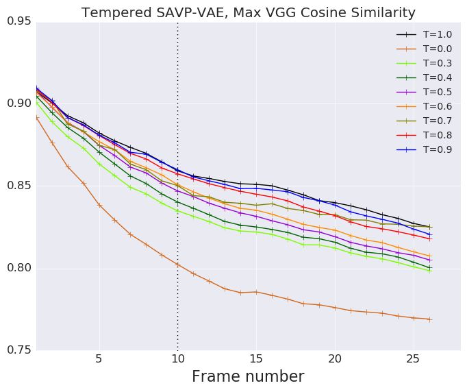
Published as a conference paper at ICLR 2020

of past observations (Ranzato et al., 2014; Srivastava et al., 2015; Vondrick et al., 2015; Xingjian
et al., 2015; Boots et al., 2014). Specifically, we propose a new class of video prediction models
that can provide exact likelihoods, generate diverse stochastic futures, and accurately synthesize
realistic and high-quality video frames. The main idea behind our approach is to extend flow-based
generative models (Dinh et al., 2014; 2016) into the setting of conditional video prediction. To our
knowledge, flow-based models have been applied only to generation of non-temporal data, such as
images (Kingma & Dhariwal, 2018), and to audio sequences (Prenger et al., 2018). Conditional
generation of videos presents its own unique challenges: the high dimensionality of video sequences
makes them difficult to model as individual datapoints. Instead, we learn a latent dynamical system
model that predicts future values of the flow model’s latent state. This induces Markovian dynamics
on the latent state of the system, replacing the standard unconditional prior distribution. We further
describe a practically applicable architecture for flow-based video prediction models, inspired by the
Glow model for image generation (Kingma & Dhariwal, 2018), which we call VideoFlow.
Our empirical results show that VideoFlow achieves results that are competitive with the state-of-
the-art in stochastic video prediction on the action-free BAIR dataset, with quantitative results that
rival the best VAE-based models. VideoFlow also produces excellent qualitative results, and avoids
many of the common artifacts of models that use pixel-level mean-squared-error for training (e.g.,
blurry predictions), without the challenges associated with training adversarial models. Compared
to models based on pixel-level autoregressive prediction, VideoFlow achieves substantially faster
test-time image synthesis 1 , making it much more practical for applications that require real-time
prediction, such as robotic control (Finn & Levine, 2017). Finally, since VideoFlow directly optimizes
the likelihood of training videos, without relying on a variational lower bound, we can evaluate its
performance directly in terms of likelihood values.

2    R ELATED W ORK

Early work on prediction of future video frames focused on deterministic predictive models (Ranzato
et al., 2014; Srivastava et al., 2015; Vondrick et al., 2015; Xingjian et al., 2015; Boots et al., 2014).
Much of this research on deterministic models focused on architectural changes, such as predicting
high-level structure (Villegas et al., 2017b), energy-based models (Xie et al., 2017), generative cooper-
ative nets (Xie et al., 2020), ABPTT (Xie et al., 2019), incorporating pixel transformations (Finn et al.,
2016; De Brabandere et al., 2016; Liu et al., 2017) and predictive coding architectures (Lotter et al.,
2017), as well as different generation objectives (Mathieu et al., 2016; Vondrick & Torralba, 2017;
Walker et al., 2015) and disentangling representations (Villegas et al., 2017a; Denton & Birodkar,
2017). With models that can successfully model many deterministic environments, the next key
challenge is to address stochastic environments by building models that can effectively reason over
uncertain futures. Real-world videos are always somewhat stochastic, either due to events that are
inherently random, or events that are caused by unobserved or partially observable factors, such as
off-screen events, humans and animals with unknown intentions, and objects with unknown physical
properties. In such cases, since deterministic models can only generate one future, these models
either disregard potential futures or produce blurry predictions that are the superposition or averages
of possible futures.
A variety of methods have sought to overcome this challenge by incorporating stochasticity, via three
types of approaches: models based on variational auto-encoders (VAEs) (Kingma & Welling, 2013;
Rezende et al., 2014), generative adversarial networks (Goodfellow et al., 2014), and autoregressive
models (Hochreiter & Schmidhuber, 1997; Graves, 2013; van den Oord et al., 2016b;c; Van Den Oord
et al., 2016).
Among these models, techniques based on variational autoencoders which optimize an evidence
lower bound on the log-likelihood have been explored most widely (Babaeizadeh et al., 2017; Denton
& Fergus, 2018; Lee et al., 2018; Xue et al., 2016; Li et al., 2018). To our knowledge, the only
prior class of video prediction models that directly maximize the log-likelihood of the data are auto-
regressive models (Hochreiter & Schmidhuber, 1997; Graves, 2013; van den Oord et al., 2016b;c;
Van Den Oord et al., 2016), that generate the video one pixel at a time (Kalchbrenner et al., 2017).
However, synthesis with such models is typically inherently sequential, making synthesis substantially
    1
      We generate 64x64 videos of 20 frames in less than 3.5 seconds on a NVIDIA P100 GPU as compared to
the fastest autoregressive model for video (Reed et al., 2017) that generates a frame every 3 seconds

                                                    2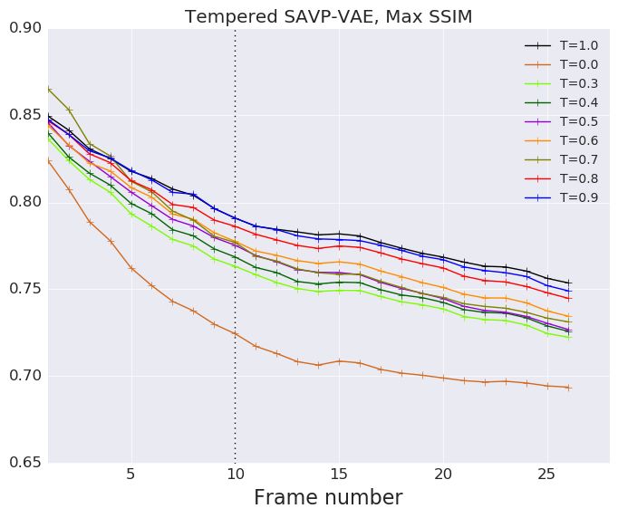
Published as a conference paper at ICLR 2020

                                                                   z0          z1                zT

                                                                         (3)         (3)               (3)
                                                                        z0          z1     ...        zT

                                                                         (2)         (2)               (2)
                                                                        z0          z1     ...        zT

                z   z(1)     z(2)              z(L−1)    z(L)
                                                                         (1)         (1)               (1)
                                                                        z0          z1     ...        zT

           x                           ...                              x0          x1     ...        xT

Figure 1: Left: Multi-scale prior The flow model uses a multi-scale architecture using several levels of
stochastic variables. Right: Autoregressive latent-dynamic prior The input at each timestep xt is encoded
                                               (1)          (L)
into multiple levels of stochastic variables (zt , . . . , zt ). We model those levels through a sequential process
Q Q        (l)    (l)  (>l)
   t  l p(zt | z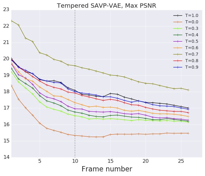
Published as a conference paper at ICLR 2020

4.1   I NVERTIBLE MULTI - SCALE ARCHITECTURE

We first briefly describe the invertible transformations used in the multi-scale architecture to infer
   (l)
{zt }L l=1 = fθ (xt ) and refer to (Dinh et al., 2016; Kingma & Dhariwal, 2018) for more details. For
convenience, we omit the subscript t in this subsection. We choose invertible transformations whose
Jacobian determinant in Equation 1 is simple to compute, that is a triangular matrix, diagonal matrix
or a permutation matrix as explored in prior work (Rezende & Mohamed, 2015; Deco & Brauer,
1995). For permutation matrices, the Jacobian determinant is one and for triangular and diagonal
Jacobian matrices, the determinant is simply the product of diagonal terms.

       • Actnorm: We apply a learnable per-channel scale and shift with data-dependent initialization.
       • Coupling: We split the input y equally across channels to obtain y1 and y2 . We compute
         z2 = f (y1 ) ∗ y2 + g(y1 ) where f and g are deep networks. We concat y1 and z2 across
         channels.
       • SoftPermute: We apply a 1x1 convolution that preserves the number of channels.
       • Squeeze: We reshape the input from H × W × C to H/2 × W/2 × 4C which allows the
         flow to operate on a larger receptive field.

We infer the latent variable z (l) at level l using:
                        Flow(y) = Coupling(SoftPermute(Actnorm(y)))) × N                                (2)
                        Flowl (y) = Split(Flow(Squeeze(y)))                                             (3)
                        (h(>l) , zl ) ← Flowl (h(>l−1) )                                                (4)

where N is the number of steps of flow. In Equation (3), via Split, we split the output of Flow equally
across channels into h(>l) , the input to Flow(l+1) (.) and z (l) , the latent variable at level l. We, thus
enable the flows at higher levels to operate on a lower number of dimensions and larger scales. When
l = 1, h(>l−1) is just the input frame x and for l = L we omit the Split operation. Finally, our
multi-scale architecture fθ (xt ) is a composition of the flows at multiple levels from l = 1 . . . L from
                                             (l)
which we obtain our latent variables i.e {zt }L  l=1 .

4.2   AUTOREGRESSIVE LATENT DYNAMICS MODEL

We use the multi-scale architecture described above to infer the set of corresponding latent variables
                                           (l)
for each individual frame of the video: {zt }L l=1 = fθ (xt ); see Figure 1 for an illustration. As in
Equation (1), we need to choose a form of latent prior pθ (z). We use the following autoregressive
factorization for the latent prior:
                                                           T
                                                           Y
                                                pθ (z) =           pθ (zt |z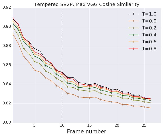
Published as a conference paper at ICLR 2020

              Model          Fooling rate
            SAVP-VAE           16.4 %
            VideoFlow          31.8 %
              SV2P             17.5 %
Table 1: We compare the realism of the generated trajec-
tories using a real-vs-fake 2AFC Amazon Mechanical
Turk with SAVP-VAE and SV2P.                               Figure 2: We condition the VideoFlow model with
                                                           the frame at t = 1 and display generated trajectories
                                                           at t = 2 and t = 3 for three different shapes.

where N Nθ (.) is a deep 3-D residual network (He et al., 2015) augmented with dilations and gated
activation units and modified to predict the mean and log-scale. We describe the architecture and our
ablations of the architecture in Section D and E of the appendix.
In summary, the log-likelhood objective of Equation (1) has two parts. The invertible multi-scale
                           PK
architecture contributes i=1 log | det(dhi /dhi−1 )| via the sum of the log Jacobian determinants
of the invertible transformations mapping the video {xt }Tt=1 to {zt }Tt=1 ; the latent dynamics model
contributes log pθ (z), i.e Equation (5). We jointly learn the parameters of the multi-scale architecture
and latent dynamics model by maximizing this objective.
Note that in our architecture we have chosen to let the prior pθ (z), as described in eq. (5), model
temporal dependencies in the data, while constraining the flow gθ to act on separate frames of video.
We have experimented with using 3-D convolutional flows, but found this to be computationally
overly expensive compared to an autoregressive prior; in terms of both number of operations and
number of parameters. Further, due to memory limits, we found it only feasible to perform SGD
with a small number of sequential frames per gradient step. In case of 3-D convolutions, this would
make the temporal dimension considerably smaller during training than during synthesis; this would
change the model’s input distribution between training and synthesis, which often leads to various
temporal artifacts. Using 2-D convolutions in our flow fθ with autoregressive priors, allows us to
synthesize arbitrarily long sequences without introducing such artifacts.

5     E XPERIMENTS

All our generated videos and qualitative results can be viewed at this website. In the generated videos,
a border of blue represents the conditioning frame, while a border of red represents the generated
frames.

5.1   V IDEO MODELLING WITH THE S TOCHASTIC M OVEMENT DATASET

We use VideoFlow to model the Stochastic Movement Dataset used in (Babaeizadeh et al., 2017).
The first frame of every video consists of a shape placed near the center of a 64x64x3 resolution gray
background with its type, size and color randomly sampled. The shape then randomly moves in one
of eight directions with constant speed. (Babaeizadeh et al., 2017) show that conditioned on the first
frame, a deterministic model averages out all eight possible directions in pixel space. Since the shape
moves with a uniform speed, we should be able to model the position of the shape at the (t + 1)th step
using only the position of the shape at the tth step. Using this insight, we extract random temporal
patches of 2 frames from each video of 3 frames. We then use VideoFlow to maximize the log-
likelihood of the second frame given the first, i.e the model looks back at just one frame. We observe
that the bits-per-pixel on the holdout set reduces to a very low 0.04 bits-per-pixel for this model. On
generating videos conditioned on the first frame, we observe that the model consistently predicts the
future trajectory of the shape to be one of the eight random directions. We compare our model with
two state-of-the-art stochastic video generation models SV2P and SAVP-VAE (Babaeizadeh et al.,
2017; Lee et al., 2018) using their Tensor2Tensor implementation (Vaswani et al., 2018). We assess
the quality of the generated videos using a real vs fake Amazon Mechanical Turk test. In the test, we
inform the rater that a "real" trajectory is one in which the shape is consistent in color and congruent

                                                      5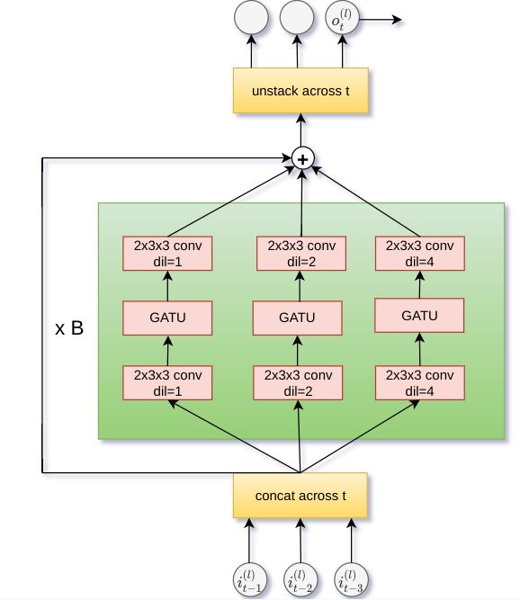
Published as a conference paper at ICLR 2020

              Model         Bits-per-pixel
            VideoFlow            1.87
            SAVP-VAE           ≤ 6.73
              SV2P             ≤ 6.78
Table 2: Left: We report the average bits-per-pixel
across 10 target frames with 3 conditioning frames for       Figure 3: We measure realism using a 2AFC test
the BAIR action-free dataset.                                and diversity using mean pairwise cosine distance
                                                             between generated samples in VGG perceptual
                                                             space.

throughout the video. We show that VideoFlow outperforms the baselines in terms of fooling rate in
Table 1 consistently generating plausible "real" trajectories at a greater rate.

5.2    V IDEO M ODELING WITH THE BAIR DATASET

We use the action-free version of the BAIR robot pushing dataset (Ebert et al., 2017) that contain
videos of a Sawyer robotic arm with resolution 64x64. In the absence of actions, the task of
video generation is completely unsupervised with multiple plausible trajectories due to the partial
observability of the environment and stochasticity of the robot actions. We train the baseline models,
SAVP-VAE, SV2P and SVG-LP to generate 10 target frames, conditioned on 3 input frames. We
extract random temporal patches of 4 frames, and train VideoFlow to maximize the log-likelihood of
the 4th frame given a context of 3 past frames. We, thus ensure that all models have seen a total of 13
frames during training.
Bits-per-pixel: We estimated the variational bound of the bits-per-pixel on the test set, via importance
sampling, from the posteriors for the SAVP-VAE and SV2P models. We find that VideoFlow
outperforms these models on bits-per-pixel and report these values in Table 2. We attribute the high
values of bits-per-pixel of the baselines to their optimization objective. They do not optimize the
variational bound on the log-likelihood directly due to the presence of a β 6= 1 term in their objective
and scheduled sampling (Bengio et al., 2015).

Figure 4: For a given set of conditioning frames on the BAIR action-free we sample 100 videos from each of
the stochastic video generation models. We choose the video closest to the ground-truth on the basis of PSNR,
SSIM and VGG perceptual metrics and report the best possible value for each of these metrics. All the models
were trained using ten target frames but are tested to generate 27 frames. For all the reported metrics, higher is
better.

Accuracy of the best sample: The BAIR robot-pushing dataset is highly stochastic and the number
of plausible futures are high. Each generated video can be super realistic, can represent a plausible
future in theory but can be far from the single ground truth video perceptually. To partially overcome
this, we follow the metrics proposed in prior work (Babaeizadeh et al., 2017; Lee et al., 2018; Denton
& Fergus, 2018) to evaluate our model. For a given set of conditioning frames in the BAIR action-free
test-set, we generate 100 videos from each of the stochastic models. We then compute the closest of
these generated videos to the ground truth according to three different metrics, PSNR (Peak Signal to

                                                        6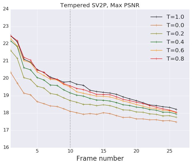
Published as a conference paper at ICLR 2020

Noise Ratio), SSIM (Structural Similarity) (Wang et al., 2004) and cosine similarity using features
obtained from a pretrained VGG network (Dosovitskiy & Brox, 2016; Johnson et al., 2016) and
report our findings in Figure 4. This metric helps us understand if the true future lies in the set of all
plausible futures according to the video model.
In prior work, (Lee et al., 2018; Babaeizadeh et al., 2017; Denton & Fergus, 2018) effectively tune
the pixel-level variance as a hyperparameter and sample from a deterministic decoder. They obtain
training stabiltiy and improve sample quality by removing pixel-level noise using this procedure.
We can remove pixel-level noise in our VideoFlow model resulting in higher quality videos at the
cost of diversity by sampling videos at a lower temperature, analogous to the procedure in (Kingma
& Dhariwal, 2018). For a network trained with additive coupling layers, we can sample the tth
frame xt from P (xt |x
Published as a conference paper at ICLR 2020

                                        # Frames Seen: Training
                           Conditioning          3        3              3         2
                              Total             13       13              13        16
                                          # Frames: Evaluation
                           Ground truth             3          3         2         2
                              Total                13         16         16        16
                             Model                               FVD
                        VideoFlow (T=0.8)        95±4       127±3      131±5       -
                        VideoFlow (T=1.0)        149±6      221±8      251±7       -
                              SAVP                 -          -          -        116
                              SV2P                 -          -          -        263
Table 3: Fréchet Video Distance:. We report the mean and standard deviation across 5 runs for 3 different
frame settings. Results are not directly comparable across models due to the differences between the total
number of frames seen during training and the number of conditioning frames.

model on a total of 13 frames with 3 conditioning frames, making our results not directly comparable
to theirs. We evaluate FVD for both shorter and longer rollouts in Table 3. We show that, even in the
settings that are disadvantageous to VideoFlow, where we compute the FVD on a total of 16 frames,
when trained on just 13 frames, VideoFlow performs comparable to SAVP.

5.3   L ATENT SPACE INTERPOLATION

BAIR robot pushing dataset: We encode the first input frame and the last target frame into the
latent space using our trained VideoFlow encoder and perform interpolations. We find that the motion
of the arm is interpolated in a temporally cohesive fashion between the initial and final position.
Further, we use the multi-level latent representation to interpolate representations at a particular level
while keeping the representations at other levels fixed. We find that the bottom level interpolates the
motion of background objects which are at a smaller scale while the top level interpolates the arm
motion.

Figure 6: Left: We display interpolations between a) a small blue rectangle and a large yellow rectangle b) a
small blue circle and a large yellow circle. Right: We display interpolations between the first input frame and
the last target frame of two test videos in the BAIR robot pushing dataset.

Stochastic Movement Dataset: We encode two different shapes with their type fixed but a different
size and color into the latent space. We observe that the size of the shape gets smoothly interpolated.
During training, we sample the colors of the shapes from a uniform discrete distribution which is
reflected in our experiments. We observe that all the colors in the interpolated space lie in the set of
colors in the training set.

5.4   L ONGER PREDICTIONS

We generate 100 frames into the future using our model trained on 13 frames with a temperature of
0.5 and display our results in Figure 7. On the top, even 100 frames into the future, the generated
frames remain in the image manifold maintaining temporal consistency. In the presence of occlusions,

                                                        8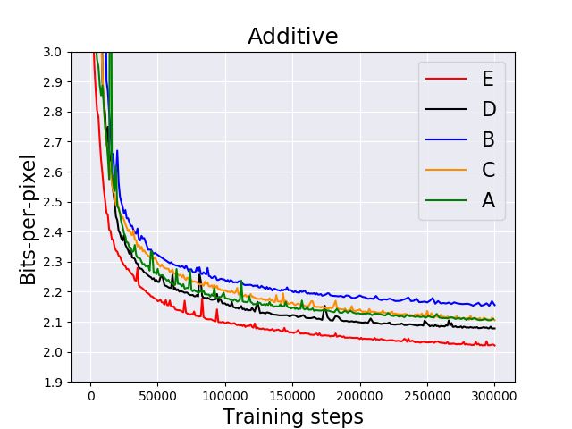
Published as a conference paper at ICLR 2020

Figure 7: Left: We generate 100 frames into the future with a temperature of 0.5. The top and bottom row
correspond to generated videos in the absence and presence of occlusions respectively. Right: We use VideoFlow
to detect the plausibility of a temporally inconsistent frame to occur in the immediate future.

the arm remains super-sharp but the background objects become noisier and blurrier. Our VideoFlow
model has a bijection between the zt and xt meaning that the latent state zt cannot store information
other than that present in the frame xt . This, in combination with the Markovian assumption in our
latent dynamics means that the model can forget objects if they have been occluded for a few frames.
In future work, we would address this by incorporating longer memory in our VideoFlow model; for
example by parameterizing N Nθ () as a recurrent neural network in our autoregressive prior (eq. 8)
or using more memory-efficient backpropagation algorithms for invertible neural networks (Gomez
et al., 2017).

5.5   O UT- OF - SEQUENCE DETECTION

We use our trained VideoFlow model, conditioned on 3 frames as explained in Section 5.2, to detect
the plausibility of a temporally inconsistent frame to occur in the immediate future. We condition
the model on the first three frames of a test-set video X
Published as a conference paper at ICLR 2020

R EFERENCES
Mohammad Babaeizadeh, Chelsea Finn, Dumitru Erhan, Roy H Campbell, and Sergey Levine.
 Stochastic variational video prediction. arXiv preprint arXiv:1710.11252, 2017.
Samy Bengio, Oriol Vinyals, Navdeep Jaitly, and Noam Shazeer. Scheduled sampling for sequence
  prediction with recurrent neural networks. In Advances in Neural Information Processing Systems,
  pp. 1171–1179, 2015.
Byron Boots, Arunkumar Byravan, and Dieter Fox. Learning predictive models of a depth camera &
  manipulator from raw execution traces. In International Conference on Robotics and Automation
  (ICRA), 2014.
Bert De Brabandere, Xu Jia, Tinne Tuytelaars, and Luc Van Gool. Dynamic filter networks. In Neural
  Information Processing Systems (NIPS), 2016.
Gustavo Deco and Wilfried Brauer. Higher order statistical decorrelation without information loss.
 Advances in Neural Information Processing Systems, pp. 247–254, 1995.
Emily Denton and Vighnesh Birodkar. Unsupervised learning of disentangled representations from
 video. arXiv preprint arXiv:1705.10915, 2017.
Emily Denton and Rob Fergus. Stochastic video generation with a learned prior. arXiv preprint
 arXiv:1802.07687, 2018.
Laurent Dinh, David Krueger, and Yoshua Bengio. Nice: non-linear independent components
  estimation. arXiv preprint arXiv:1410.8516, 2014.
Laurent Dinh, Jascha Sohl-Dickstein, and Samy Bengio. Density estimation using Real NVP. arXiv
  preprint arXiv:1605.08803, 2016.
Alexey Dosovitskiy and Thomas Brox. Generating images with perceptual similarity metrics based
  on deep networks. In Advances in Neural Information Processing Systems, pp. 658–666, 2016.
Frederik Ebert, Chelsea Finn, Alex X Lee, and Sergey Levine. Self-supervised visual planning with
  temporal skip connections. arXiv preprint arXiv:1710.05268, 2017.
Chelsea Finn and Sergey Levine. Deep visual foresight for planning robot motion. In International
  Conference on Robotics and Automation (ICRA), 2017.
Chelsea Finn, Ian Goodfellow, and Sergey Levine. Unsupervised learning for physical interaction
  through video prediction. In Advances in Neural Information Processing Systems, 2016.
Aidan N Gomez, Mengye Ren, Raquel Urtasun, and Roger B Grosse. The reversible residual network:
  Backpropagation without storing activations. In Advances in Neural Information Processing
  Systems, pp. 2211–2221, 2017.
Ian Goodfellow, Jean Pouget-Abadie, Mehdi Mirza, Bing Xu, David Warde-Farley, Sherjil Ozair,
  Aaron Courville, and Yoshua Bengio. Generative adversarial nets. In Advances in Neural
  Information Processing Systems, pp. 2672–2680, 2014.
Alex Graves. Generating sequences with recurrent neural networks. arXiv preprint arXiv:1308.0850,
  2013.
Kaiming He, Xiangyu Zhang, Shaoqing Ren, and Jian Sun. Deep residual learning for image
  recognition. arXiv preprint arXiv:1512.03385, 2015.
Martin Heusel, Hubert Ramsauer, Thomas Unterthiner, Bernhard Nessler, and Sepp Hochreiter. Gans
 trained by a two time-scale update rule converge to a local nash equilibrium. In Advances in neural
 information processing systems, pp. 6626–6637, 2017.
Sepp Hochreiter and Jürgen Schmidhuber. Long Short-Term Memory. Neural computation, 9(8):
  1735–1780, 1997.

                                                10
Published as a conference paper at ICLR 2020
Catalin Ionescu, Dragos Papava, Vlad Olaru, and Cristian Sminchisescu. Human3. 6m: Large scale
datasets and predictive methods for 3d human sensing in natural environments. IEEE transactions
on pattern analysis and machine intelligence, 36(7):1325–1339, 2014.
Justin Johnson, Alexandre Alahi, and Li Fei-Fei. Perceptual losses for real-time style transfer and
super-resolution. In European Conference on Computer Vision, pp. 694–711. Springer, 2016.
Nal Kalchbrenner, Aäron van den Oord, Karen Simonyan, Ivo Danihelka, Oriol Vinyals, Alex Graves,
and Koray Kavukcuoglu. Video pixel networks. International Conference on Machine Learning
(ICML), 2017.
Diederik P Kingma and Max Welling. Auto-encoding variational Bayes. Proceedings of the 2nd
International Conference on Learning Representations, 2013.
Durk P Kingma and Prafulla Dhariwal. Glow: Generative flow with invertible 1x1 convolutions. In
Advances in Neural Information Processing Systems, pp. 10236–10245, 2018.
Alex Krizhevsky, Ilya Sutskever, and Geoff Hinton. Imagenet classification with deep convolutional
neural networks. In Advances in Neural Information Processing Systems 25, pp. 1106–1114, 2012.
Alex X Lee, Richard Zhang, Frederik Ebert, Pieter Abbeel, Chelsea Finn, and Sergey Levine.
Stochastic adversarial video prediction. arXiv preprint arXiv:1804.01523, 2018.
Yijun Li, Chen Fang, Jimei Yang, Zhaowen Wang, Xin Lu, and Ming-Hsuan Yang. Flow-grounded
spatial-temporal video prediction from still images. In Proceedings of the European Conference
on Computer Vision (ECCV), pp. 600–615, 2018.
Ziwei Liu, Raymond Yeh, Xiaoou Tang, Yiming Liu, and Aseem Agarwala. Video frame synthesis
using deep voxel flow. International Conference on Computer Vision (ICCV), 2017.
William Lotter, Gabriel Kreiman, and David Cox. Deep predictive coding networks for video
prediction and unsupervised learning. International Conference on Learning Representations
(ICLR), 2017.
Michael Mathieu, Camille Couprie, and Yann LeCun. Deep multi-scale video prediction beyond
mean square error. International Conference on Learning Representations (ICLR), 2016.
Volodymyr Mnih, Koray Kavukcuoglu, David Silver, Alex Graves, Ioannis Antonoglou, Daan
Wierstra, and Martin Riedmiller. Playing Atari with deep reinforcement learning. arXiv preprint
arXiv:1312.5602, 2013.
Ryan Prenger, Rafael Valle, and Bryan Catanzaro. Waveglow: A flow-based generative network
for speech synthesis. CoRR, abs/1811.00002, 2018. URL http://arxiv.org/abs/1811.
00002.
Prajit Ramachandran, Tom Le Paine, Pooya Khorrami, Mohammad Babaeizadeh, Shiyu Chang, Yang
Zhang, Mark A Hasegawa-Johnson, Roy H Campbell, and Thomas S Huang. Fast generation for
convolutional autoregressive models. arXiv preprint arXiv:1704.06001, 2017.
MarcAurelio Ranzato, Arthur Szlam, Joan Bruna, Michael Mathieu, Ronan Collobert, and Sumit
Chopra. Video (language) modeling: a baseline for generative models of natural videos. arXiv
preprint arXiv:1412.6604, 2014.
Scott Reed, Aäron van den Oord, Nal Kalchbrenner, Sergio Gómez Colmenarejo, Ziyu Wang, Dan
Belov, and Nando de Freitas. Parallel multiscale autoregressive density estimation. arXiv preprint
arXiv:1703.03664, 2017.
Danilo Rezende and Shakir Mohamed. Variational inference with normalizing flows. In Proceedings
of The 32nd International Conference on Machine Learning, pp. 1530–1538, 2015.
Danilo J Rezende, Shakir Mohamed, and Daan Wierstra. Stochastic backpropagation and approximate
inference in deep generative models. In Proceedings of the 31st International Conference on
Machine Learning (ICML-14), pp. 1278–1286, 2014.
11Published as a conference paper at ICLR 2020
David Silver, Julian Schrittwieser, Karen Simonyan, Ioannis Antonoglou, Aja Huang, Arthur Guez,
Thomas Hubert, Lucas Baker, Matthew Lai, Adrian Bolton, et al. Mastering the game of go without
human knowledge. Nature, 550(7676):354, 2017.
Nitish Srivastava, Elman Mansimov, and Ruslan Salakhudinov. Unsupervised learning of video
representations using lstms. In International Conference on Machine Learning, 2015.
Thomas Unterthiner, Sjoerd van Steenkiste, Karol Kurach, Raphael Marinier, Marcin Michalski, and
Sylvain Gelly. Towards accurate generative models of video: A new metric & challenges, 2018.
Aaron Van Den Oord, Sander Dieleman, Heiga Zen, Karen Simonyan, Oriol Vinyals, Alex Graves,
Nal Kalchbrenner, Andrew Senior, and Koray Kavukcuoglu. Wavenet: A generative model for raw
audio. arXiv preprint arXiv:1609.03499, 2016.
Aaron van den Oord, Nal Kalchbrenner, Lasse Espeholt, Oriol Vinyals, Alex Graves, et al. Conditional
image generation with PixelCNN decoders. In Advances in Neural Information Processing Systems,
pp. 4790–4798, 2016a.
Aaron van den Oord, Nal Kalchbrenner, and Koray Kavukcuoglu. Pixel recurrent neural networks.
arXiv preprint arXiv:1601.06759, 2016b.
Aaron van den Oord, Nal Kalchbrenner, Oriol Vinyals, Lasse Espeholt, Alex Graves, and Ko-
ray Kavukcuoglu. Conditional image generation with PixelCNN decoders. arXiv preprint
arXiv:1606.05328, 2016c.
Ashish Vaswani, Noam Shazeer, Niki Parmar, Jakob Uszkoreit, Llion Jones, Aidan N Gomez, Łukasz
Kaiser, and Illia Polosukhin. Attention is all you need. In Advances in Neural Information
Processing Systems, pp. 5998–6008, 2017.
Ashish Vaswani, Samy Bengio, Eugene Brevdo, Francois Chollet, Aidan N Gomez, Stephan Gouws,
Llion Jones, Łukasz Kaiser, Nal Kalchbrenner, Niki Parmar, et al. Tensor2tensor for neural machine
translation. arXiv preprint arXiv:1803.07416, 2018.
Ruben Villegas, Jimei Yang, Seunghoon Hong, Xunyu Lin, and Honglak Lee. Decomposing motion
and content for natural video sequence prediction. arXiv preprint arXiv:1706.08033, 2017a.
Ruben Villegas, Jimei Yang, Yuliang Zou, Sungryull Sohn, Xunyu Lin, and Honglak Lee. Learning
to generate long-term future via hierarchical prediction. In Proceedings of the 34th International
Conference on Machine Learning-Volume 70, pp. 3560–3569. JMLR. org, 2017b.
Carl Vondrick and Antonio Torralba. Generating the future with adversarial transformers. In Computer
Vision and Pattern Recognition (CVPR), 2017.
Carl Vondrick, Hamed Pirsiavash, and Antonio Torralba. Anticipating the future by watching
unlabeled video. arXiv preprint arXiv:1504.08023, 2015.
Jacob Walker, Abhinav Gupta, and Martial Hebert. Dense optical flow prediction from a static image.
In International Conference on Computer Vision (ICCV), 2015.
Zhou Wang, Alan C Bovik, Hamid R Sheikh, and Eero P Simoncelli. Image quality assessment: from
error visibility to structural similarity. IEEE transactions on image processing, 2004.
Jianwen Xie, Song-Chun Zhu, and Ying Nian Wu. Synthesizing dynamic patterns by spatial-temporal
generative convnet. In The IEEE Conference on Computer Vision and Pattern Recognition (CVPR),
July 2017.
Jianwen Xie, Ruiqi Gao, Zilong Zheng, Song-Chun Zhu, and Ying Nian Wu. Learning dynamic gen-
erator model by alternating back-propagation through time. Proceedings of the AAAI Conference
on Artificial Intelligence, 33:5498âĂŞ5507, Jul 2019. ISSN 2159-5399. doi: 10.1609/aaai.v33i01.
33015498. URL http://dx.doi.org/10.1609/aaai.v33i01.33015498.
Jianwen Xie, Yang Lu, Ruiqi Gao, Song-Chun Zhu, and Ying Nian Wu. Cooperative training
of descriptor and generator networks. IEEE Transactions on Pattern Analysis and Machine
Intelligence, 42(1):27âĂŞ45, Jan 2020. ISSN 1939-3539. doi: 10.1109/tpami.2018.2879081. URL
http://dx.doi.org/10.1109/TPAMI.2018.2879081.
12Published as a conference paper at ICLR 2020
SHI Xingjian, Zhourong Chen, Hao Wang, Dit-Yan Yeung, Wai-Kin Wong, and Wang-chun Woo.
Convolutional lstm network: A machine learning approach for precipitation nowcasting. In
Advances in Neural Information Processing Systems, 2015.
Tianfan Xue, Jiajun Wu, Katherine Bouman, and Bill Freeman. Visual dynamics: Probabilistic future
frame synthesis via cross convolutional networks. In Advances in Neural Information Processing
Systems, 2016.
Richard Zhang, Phillip Isola, Alexei A Efros, Eli Shechtman, and Oliver Wang. The unreasonable
effectiveness of deep features as a perceptual metric. arXiv preprint, 2018.
A M OVING MNIST - Q UALITATIVE E XPERIMENTS
Figure 8: We display ten frame rollouts conditioned on a single frame on the Moving MNIST dataset.
Similar to the Stochastic Movement Dataset as described in Section 5.1, we extract random temporal
patches of 2 frames on the Moving MNIST dataset (Srivastava et al., 2015). We train our VideoFlow
model to maximize the log-likelihood of the second frame, given the first. Our rollouts over 10 frames
capture realistic digit movement.
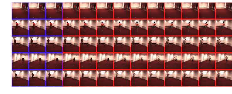
B H UMAN 3.6M - Q UALITATIVE E XPERIMENTS
We model the Human3.6M dataset (Ionescu et al., 2014), by maximizing the log-likelihood of the
4th frame given the first three frames, in a random temporal patch of 4 frames. We observe that on
this dataset, our model fails to capture reasonable human motion. We hope that by increasing model
capacity and using more expressive priors, we can acheive better performance on this dataset in the
future.
C D ISCRETIZATION AND U NIFORM QUANTIZATION
Let D = {x(i) }N i=1 be our dataset of i.i.d. observations of a random variable x with an unknown
true distribution p∗ (x). Our data consist of 8-bit videos, with each dimension rescaled to the domain
[0, 255/256]. We add a small amount of uniform noise to the data, u ∼ U(0, 1/256.), matching its
discretization level (Dinh et al., 2016; Kingma & Dhariwal, 2018). Let q(x) be the resulting empirical
distribution corresponding to this scaling and addition of noise. Note that additive noise is required
to prevent q(x) from having infinite densities at the datapoints, which can result in ill-behaved
optimization of the log-likelihood; it also allows us to recast maximization of the log-likelihood as
minimization of a KL divergence.
13Published as a conference paper at ICLR 2020
Figure 9: We display ten frame rollouts conditioned on 3 frames on the Human3.6M dataset.
D R ESIDUAL NETWORK ARCHITECTURE
(l) (>l)
Here we’ll describe the architecture for the residual network N Nθ () that maps zl)
to (µt , log σt ) (Left: Figure 10). As shown in the left of Figure 10, let ht be the
(>l)
tensor representing zt after the split operation between levels in the multi-scale architec-
(>l)
ture. We apply a 1 × 1 convolution over ht and concatenate this across channels to
each latent from the previous time-step and the same-level independently. In this way, we
(>l) (l) (>l) (l) (>l) (l)
obtain ((W ht ; zt−1 ), (W ht ; zt−2 ) . . . (W ht ; zt−n )). We transform these values into
(l) (l)
(µt , log σt ) via a stack of residual blocks. We obtain a reduction in parameter count by sharing
parameters across every 2 time-steps via 3-D convolutions in our residual blocks.
As shown in the right of Figure 10, each 3-D residual block consists of three layers. The first layer
has a filter size of 2x3x3 with 512 output channels followed by a ReLU activation. The second layer
has two 1 × 1 × 1 convolutions via the Gated Activation Unit Van Den Oord et al. (2016); van den
Oord et al. (2016a). The third layer has a filter size of 2 × 3 × 3 with the number of output channels
determined by the level. This block is replicated three times in parallel, with dilation rates 1, 2 and 4,
after which the results of each block, in addition to the input of the residual block, are summed.
The first two layers are initialized using a Gaussian distribution and the last layer is initialized
to zeroes. In that way, the residual network behaves as an identity network during initialization
allowing stable optimization. After applying a sequence of residual blocks, we use the last temporal
activation that should capture all context. We apply a final 1 × 1 convolution to this activation to
(l) (l) (l) (l) (l)
obtain (∆zt , log σt ). We then add ∆zt to zt−1 to a temporal skip connection to output µt . This
way, the network learns to predict the change in latent variables for a given level. We have provided
visualizations of the network architecture in this website
E A BLATION S TUDIES
Through an ablation study, we experimentally evaluate the importance of the following components
of our VideoFlow model: (1) the use of temporal skip connections, (2) the use Gated Activation Unit
(GATU) instead of ReLUs in the residual network and (3) the use of dilations in N Nθ () in Section D
We start with a VideoFlow model with 256 channels in the coupling layer, 16 steps of flow and
remove the components mentioned above to create our baseline. We use four different combinations
of our components (described in Fig. 11) and keep the rest of the hyperparameters fixed across those
combinations. For each combination we plot the mean bits-per-pixel on the holdout BAIR-action
14Published as a conference paper at ICLR 2020
(l) (l)
Figure 10: Left: We predict a gaussian distribution over zt via a 3-D Residual network conditioned on zl)
and zt . Right: Our 3-D residual network architecture is augmented with dilations and gated activation units
improving performance.
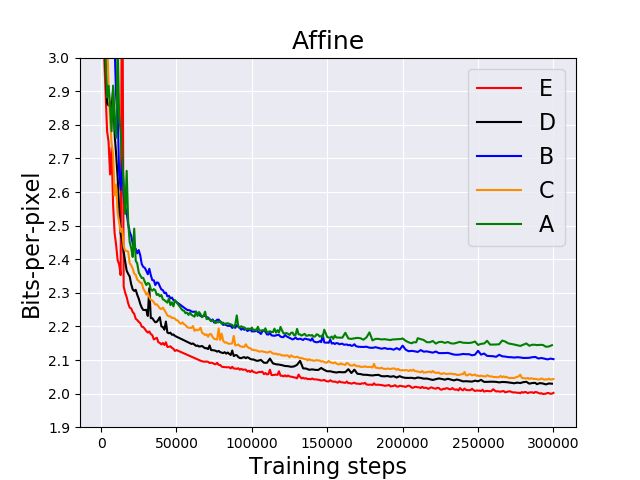
free dataset over 300K training steps for both affine and additive coupling in Figure 11. For both the
coupling layers, we observe that the VideoFlow model with all the components provide a significant
boost in bits-per-pixel over our baseline.
Figure 11: B: baseline, A: Temporal Skip Connection, C: Dilated Convolutions + GATU, D: Dilation
Convolutions + Temporal Skip Connection, E: Dilation Convolutions + Temporal Skip Connection +
GATU. We plot the holdout bits-per-pixel on the BAIR action-free dataset for different ablations of our
VideoFlow model.
We also note that other combinations—dilated convolutions + GATU (C) and dilated convolutions +
the temporal skip connection —improve over the baseline. Finally, we experienced that increasing
the receptive field in N Nθ () using dilated convolutions alone in the absence of the temporal skip
connection or the GATU makes training highly unstable.
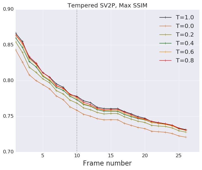
F E FFECT OF TEMPERATURE ON SAVP-VAE AND SV2P
We repeat our evaluations described in Figure 4 applying low temperature to the latent gaussian
priors of SV2P and SAVP-VAE. We empirically find that decreasing temperature from 1.0 to 0.0
monotonically decreases the performance of the VAE models. Our insight is that the VideoFlow
15Published as a conference paper at ICLR 2020
Figure 12: We repeat our evaluations described on the SV2P and SAVP-VAE model in Figure 4 using tempera-
tures from 0.0 to 1.0 while sampling from the latent gaussian prior.
model gains by low-temperature sampling due to the following reason. At lower T, we obtain a
tradeoff between a performance gain by noise removal from the background and a performance hit
due to reduced stochasticity of the robot arm. On the other hand, the VAE models have a clear but
slightly blurry background throughout from T = 1.0 to T = 0.0. Reducing T in this case, solely
reduces the stochasticity of the arm motion thus hurting performance.
G L IKELIHOOD VS Q UALITY
Figure 13: We provide a comparison between training progression (measured in the mean bits-per-pixel objective
on the test-set) and the quality of generated videos.
We show correlation between training progression (measured in bits per pixel) and quality of the
generated videos in Figure 13. We display the videos generated by conditioning on frames from the
test set for three different values of bits-per-pixel on the test-set. As we approach lower bits-per-pixel,
our VideoFlow model learns to model the structure of the arm with high quality as well as its motion
resulting in high quality video.
16Published as a conference paper at ICLR 2020
H V IDEO F LOW - BAIR H YPERPARAMETERS
H.1 Q UANTITATIVE - B ITS - PER - PIXEL
To report bits-per-pixel we use the following set of hyperparameters. We use a learning rate schedule
of linear warmup for the first 10000 steps and apply a linear-decay schedule for the last 150000 steps.
Hyperparameter Value
Flow levels 3
Flow steps per level 24
Coupling Affine
Number of coupling layer channels 512
Optimier Adam
Batch size 40
Learning rate 3e-4
Number of 3-D residual blocks 5
Number of 3-D residual channels 256
Training steps 600K
H.2 Q UALITATIVE E XPERIMENTS
For all qualitative experiments and quantitative comparisons with the baselines, we used the following
sets of hyperparameters.
Hyperparameter Value
Flow levels 3
Flow steps per level 24
Coupling Additive
Number of coupling layer channels 392
Optimier Adam
Batch size 40
Learning rate 3e-4
Number of 3-D residual blocks 5
Number of 3-D residual channels 256
Training steps 500K
I H YPERPARAMETER GRID FOR THE BASELINE VIDEO MODELS .
We train all our baseline models for 300K steps using the Adam optimizer. Our models were tuned
using the maximum VGG cosine similarity metric with the ground-truth across 100 decodes.
SAVP-VAE and SV2P: We use three values of latent loss multiplier 1e-3, 1e-4 and 1e-5. For the
SAVP-VAE model, we additionally apply linear decay on the learning rate for the last 100K steps.
SAVP-GAN: We tune the gan loss multiplier and the learning rate on a logscale from 1e-2 to 1e-4
and 1e-3 to 1e-5 respectively.
J C ORRELATION BETWEEN VGG PERCEPTUAL SIMILARITY AND
BITS - PER - PIXEL
We plot correlation between cosine similarity using a pretrained VGG network and bits-per-pixel
using our trained VideoFlow model. We compare P(X4 = Xt |XPublished as a conference paper at ICLR 2020 Figure 14: We compare P(X4 = Xt |X
You can also read